Proceedings of the 20th Annual International Conference of the IEEE Engineering in Medicine and Biology Society, Vol. 20, No 6,1998
Identification of Time-Varying Joint Dynamics Using Wavelets Guangzhi Wang and Li-Qun Zhang Sensory Motor Performance Program, Rehabilitation Institute of Chicago Depts. of Phys. Med. & Rehab., Biomed. Eng., and Orthopaedic Surgery, Northwestern University Chicago, IL 606 11, USA.
[email protected] Abstract-A wavelet-based method was investigated to identify time-varying properties of joint dynamics. Wavelet decomposition was used to expand each timevarying coefficient of an autoregressive with exogenous input (ARX) model into a finite set of basis sequences, and singular value decomposition was used to obtain more robust parameter estimates of the expansion. With a set of well-selected basis, the time-varying ARX coefficients could be well approximated by a combination of a small number of basis sequences, which simplified the identification of the time-varying parameters. The estimated time-varying A R X parameters were converted to a second-order continuous-time system characterizing joint dynamics with joint stiffness, viscosity and limb inertia. Simulation based on a time-varying joint dynamics model showed that the method tracked the time-varying system parameter closely.
short period of time, so that the identification method applied to time-invariant systems can be used. It’s obvious that this method can only track the slow change of system properties. In the current study, a wavelet-based method is used to identify time-varying properties of joint dynamics based on the data of single trial. The basic idea is to expand each timevarying coefficient into a set of basis sequences. If each coefficient can be well approximated by a combination of a small number of basis sequences, then the identification task is equivalent to estimate the parameters of the expansion, which may be easier and more accurate because of the smaller number of unknowns [3]. In this study, the wavelet was chosen as the basis sequences, which have the ability of characterizing the local change as well as global characteristics of system dynamics. Several factors affecting the identification accuracy were investigated.
I. INTRODUCTION
Joint dynamics describe the dynamic relationship between the position of a joint and the torque acting about it. Let the observed data series of the torque and joint position be a realization of a discrete time, time-varying-ARX process:
Joint stiffness, viscosity and limb inertia are important dynamic properties in the control of posture and movement. These properties reflect the dynamic relationship between the joint position and torque. A human joint performing functional tasks is a time-varying system due to the change in muscle contraction, in the reflex activities of the neuromuscular system, and in joint position. Several techniques have been used to identify joint dynamics under non-stationary conditions, including the adaptive methods, ensemble method, temporal expansion method and quasitime-invariant method [2]. However, up to date, the timevarying system identification is still a difficult problem, and each time-varying system identification method involves some special restrictions. Among these methods, the popular adaptive methods are applicable only to slow time-varying systems so that the adaptation can follow the time-varying system properties. If the coefficients change too fast, comparable to the algorithm’s convergence time, adaptive algorithm may not be able to track the system’s time evolution [3]. The ensemble methods have been used to identify the dynamics of human ankle joint during voluntary contraction and imposed movement, and some interesting result have been reported [l, 21. The difficult of this method lies in that many trials of data need to be sampled and the same deterministic time-varying conditions need to be repeated in each trial, which can be difficult to achieve over hundreds of trials. The quasi-time-invariant method assumes that the system’s dynamics do not change substantially in a
0-7803-5164-9/98/$10.00 0 1998 IEEE
11. THEORY AND METHOD
e ( n )= fa(n,k)e(n - k ) + ~ b ( n , z ) ~ ( n - z ) + e ( n )(1) k=l
I 4
where a(n, k) and b(n,l) are the time-varying coefficients which depend on discrete time instant n, e(n) and T(n) denote the joint position and torque, respectively. The residuals e(n) is assumed to be a zero mean Gaussian process with a variance of 0,”. Since the coefficient a(n,k) and b(n,l) change with n, there are (p+q)*N unknowns need to estimate for a data series of length N. It is practically impossible to recover so many unknowns based on a single sample of trial (a data series of length N) directly. To solve this problem, the number of unknowns in the above model need to be reduced. If the time-evolution of each coefficient can be approximated by a combination of a smaller number of basis sequence, then the problem is reduced to the estimation of the smaller number of unknowns. The wavelet decomposition method has been proved a powerful tool in signal and image encoding and data compression. In general, if an appropriate wavelet basis is selected, most of the coefficients of the decomposed series will be near zero, and the energy of the signal tends to concentrate on a few wavelet coefficients throughout the
3040
decomposition. In other words, most of the information about the global characteristics of the signal is retained in the lowresolution level, and the local transitions usually concentrate on a few wavelet coefficients of the high resolution level. Therefore, it is expected that the unknown coefficients a(n,k) and b(n,l) can be well approximated by a combination of a smaller number of wavelet basis sequences. The identification of coefficients a(n,k) and b(n,l) are thus equivalent to identifymg the small number of wavelet coefficients. The discrete wavelet decomposition can be based on the multi-resolution filter bank theory [4].This method separates the signal into approximation and detail components of different decomposition level. To transfer each time-varying coefficient to a set of basis sequences based on wavelets, each time-varying coefficient a(n,k) and b(n,l) can be assigned as the zero level decomposition signal and feed into the filter bank to separated into low and high resolution components. The signal decomposition and corresponding reconstruction procedure for the first three level decompositions is illustrated in Fig. 1.
Fig. 2. A filter bank with parallel structure. The symbol V and A represents sub-sampling and over-sampling, respectively. Comparing Fig. 2 with Fig. 1, the low-resolution decomposition filter branch involves an sub-sampling of 2J (J denotes the decomposition depth), and the equivalent filter can be presented as:
(z)= &(z) &(z2) ...&(z2‘1’1)) The high resolution decomposition filter branch corresponding to depth j (i=2, 3, ... , J) involves an subsampling of 2’ and an equivalent filter HIG): &‘I)
HIa) (z)=
&(z) &(z2)
...&(z zw))
(z2(i-1))
Forj=2, 3, ..., Jandforj=l:
53 52
51
H~(’)(Z)=H~(Z) The same relation occurs on the reconstruction filter bank, that is, the low-resolution reconstruction filter corresponding to depth J involves an over-sampling of 2’, and the equivalent filter is: Hd‘J’(z)= H,&) Hd(z2) ...Hfi(~’‘’-~)) The high resolution reconstruction filter branch corresponding to depth j (i = 2, 3, ... , J) involves an oversampling of 2’ and a equivalent filter &lo):
Hrl@(z)= &(z) H,o(z’) ...H~(z”-~’) Hrl(z2”’)) Forj=2, 3, ...,Jandforj=l:
52 51
(b) Fig. 1. The wavelet decomposition of one time-varying coefficient a(n,k) based on filter bank theory. Decomposition and reconstruction are shown in (a) and (b), respectively. The symbol V and A means sub-sampling and over-sampling, respectively. &, H1, and Hd, Yl denote the decomposition and reconstruction filter banks. Using Noble identities, the cascade filter bank structure of Fig.1 can be transformed into an equivalent filter bank with a parallel structure as shown in Fig. 2.
Y1‘”(z)=Hr1(z) For a fixed order k or 1 of the ARX model, the time-varying coefficient a(n,k) or b(n,l) can be transferred to the wavelet coefficients corresponding to approximate and detail components denoted by CJ and Ej (j=l, 2, ..., J), respectively. If the appropriate wavelet basis is selected, it is expected to capture the global as well as the local behavior of the timevarying coefficients a(n,k) and b(n,l) with a few levels of wavelet coefficients. Based on the above decomposition procedure, each timevarying coefficient can be reconstructed by synthesis each set of wavelet Coefficients. In general, the synthesis equation can be written as:
a , ( n , k )=
m
C
(m)
h!Jo’(n
- 2’
m)
+ i z t j . h z ! ) ( n- 2 j . m ) j=1 m
3041
If we substituting this result into the time-varying ARX model ( I ) , the regressor can be presented as the linear combination of the wavelet coefficient:
.
e ( n )= i c ~ , ( " ) ( m )h:;)(n . - 2'. m) e ( n - k) k=l m
+5
I=I m