Optics and Photonics Journal, 2013, 3, 318-321 doi:10.4236/opj.2013.32B074 Published Online June 2013 (http://www.scirp.org/journal/opj)
Image Correction Method of Color Line-Scan System Zhen-long Chen, Yu-tang Ye, Yun-cen Song, Ying Luo, Lin Liu, Juan-xiu Liu School of Opto-electronic Information, University of Electronic Science and Technology of China, Chengdu 610054, China Email:
[email protected],
[email protected] Received 2013
ABSTRACT As the development of machine vision technology, the color line-scan system is widely applied in the on-line inspection. Due to the non-uniform gray scale and color distortion of the image acquired by the system, the image correction is needed to reduce the problem of image processing and the stability system. Based on reasons mentioned above, a method that using polynomial fitting to correct the image is presented to solve the problem in this paper. The method has been used in the automatic optical inspection of PCB, and has been proved to be effective. So this method will have a potential application to the development of the color line-scan machine vision system. Keywords: Machine Vision; Automatic Optical Inspection (AOI); Color Line-scan System; White Balance; Flat-field Correction
1. Introduction
2.1. Color Correction
With the development of machine vision and automated optical inspection technology, system application (such as inspection of PCB appearance defect, color print defect detection, etc...) based on the color line-scan technology is increasingly widespread. In the color line-scan visual system, the non-uniform distribution of optical intensity, the vignetting of optical lens, and the inhomogeneity of CCD camera, will result in non-uniform grayscale and color distortion of the image acquired by the system. This can bring difficulties for the back-end image processing, so that it can have some impacts on system stability[1-9].
For Cb and Cr reflecting the luminance and chrominance of red and blue channel respectively, so the color correction need to change the image from RGB to YCbCr space. The color space transform method is shown in the formula (1).
2. Image Quality Correcting Method Color line-scan system structure is shown in Figure 1. Due to the correction method of RGB channel is basically the same, we take R channel processing as an example flat-field correction method for color image description.
lens encoder
Figure 1. Structure of color line-scan system. Copyright © 2013 SciRes.
Y 0.299 Cb 0.1687 Cr 0.5
0.587 0.3313 0.4187
R 0.5 G (1) 0.0813 B 0.114
In this method, the scope of Cr and Cb is from -127 to 127. After space transform, according to the color temperature of YCbCr space, the color cast is obtained. Base on the color cast, Cb and Cr can be corrected the best value on the basis of channel gain( Cb and Cr of white color is zero, so channel gain is getting the parameters which can adjust Cb and Cr to zero or close to zero).
2.2. Noise Eliminating We use color linear CCD image acquisition system shown in Figure 1 to do image acquisition for the standard whiteboard. In the standard whiteboard image capture experiments, we collected 1000 lines image data as uniform field images, as shown in Figure 2. In order to eliminate random noise, extract gray scale information of the R channel of the color image from Figure 2, and do average processing for the pixel values in the image’s vertical direction (i.e. the relative movement direction compare colored line array CCD camera with the scan target), obtain gradation distribution shown OPJ
Z.-L. CHEN ET AL.
in Figure 3. Seen from the Figure 3, because of the lens vignetting effect, the gradation is high in the middle and low in the ends and appears actuate distribution in the horizontal direction (i.e. the colored line array CCD camera pixel arrangement direction). At the same time, due to dark current and other factors, cause that there are many spikes noise in the vertical direction, as shown in Figure 3. Since the noise is very serious, for further analysis, firstly we need do denoising for the image. Daubechies-4 wavelet was used in experiments [10] to implement fifth decomposition. After several attempts at commissioning site, we get the final threshold value of each layer is set to about 4. The fine structure in Figure 3 is substantially filtered out and we obtain the final grayscale distribution shows in Figure 4.
319
2.3. Gray level Correction In this part, fifth-order polynomial is used to do the fitting of RGB channel's gray distribution which is after denoising. In the polynomial, x is the location of pixel, and y is the gray value of the pixel at x. The correction method is as follows. If given data are consistent with the fifth-order polynomial as the formula (2): y ( x ) a5 x a4 x a3 x a2 x a1 x a0 5
4
3
2
(2)
and the fitting points are (x1,y1),(x2,y2) and so on, so the aim of least square method is getting a set of parameters (named a5, a4, a3, a2, a1 and a0) which let sum of square of deviations to the minimum. The calculation method of sum of square of deviations is as formula (3): n
x 2 [ yn y ( xn )]2
(3)
n 1
According to matrix theory, obtaining the solution of least square method can use the formula (4).
Figure 2. The white panel's image grabbed by color line-scan system
x15 5 x2 5 xn
x14 1 a5 y1 x24 1 a4 y2 or X a y xn4 1 a0 yn
(4)
For the number of equations is greater than the number of unknowns, the solution of the matrix theory can not be obtained, so only least square solution can be obtained. So the least square solution of multinomial coefficients is shown in formula(5). (5) a X y
Figure 3. The gray distribution of the white panel's R channel.
Figure 4. The gray distribution the white panel's denoising. Copyright © 2013 SciRes.
after
Since three RGB channels of color linear CCD are relatively independent, each channel was processed as above, which can get the parameters of the actual gray level correction and the deviation value for each channel at each pixel location. Then, the correction parameters for each channel is applied to the corresponding channel of the actual image, it can realize a flat field correction processing of the color image. In this paper, in order to avoid the noise’s impact on the gradation correction, firstly denoise the uniform field, then do polynomial fitting, we get the fitting curve of gray distribution as Figure 5. Using the correction parameters to correct the image shown in Figure 2, the processed gray distribution of R channel is shown in Figure 6. According to Figure 6 we can know, the gray distribution of the white panel's R channel is improved, and more suitable for threshold segmentation and edge extracting.
3. Experimental Results Apply the parameters obtained from the correction procOPJ
Z.-L. CHEN ET AL.
320
ess to the actual collection of the PCB color image, the effect of the correction around the PCB was shown in Figure 7(a), (b) (the direction of the scanning line is the image height direction). The gray level histogram before and after corrections of R channel correspond to Figure 7 is shown in Figure 8. Figure 8(a) shows that before the correction the image grayscale distribution has more peaks and the difference is not obvious. Image processing like threshold segmentation is very difficult. With reference to Figure 7(a), we can get that this is because the whole image is dim, and more to the direction of the large field angle, the lower the pixel value will be. After corrections, the grayscale distribution tends to be high, low ends and concentrated peak became distinct, which is consistent with the entire image brightness and uniformity improved shown in Figure 7(b). After using the correction method proposed in this paper, the image quality is improved. More reliable image sources for image segmentation, cluster analysis in the subsequent processing of the system are provided. And it’s conducive to the stability of the system.
Figure 5. The fitting curve of gray distribution at R channel.
(b)processed image
Figure 7. The comparison between before and after process the PCB image.
(a) the density histogram of source image
(b) density histogram of processed image
Figure 8. The the R channel density histogram of before and after processing PCB image.
4. Conclusions
Figure 6. The processed gray distribution of R channel.
(a) source image
Copyright © 2013 SciRes.
According to the characteristics of the actual build color linear CCD image acquisition system, this article proposed a flat-field correction method of the color line image. Although processing steps of correction process is a bit much, once get the system correction factor, it can be applied in all acquired PCB images by looking up tables without taking up processing resources of the detection system and adjusting the hardware system. It’s very valuable for the actual application of PCB detection system. The method has been applied to “the superficial defect of smart printed circuit board (PCB) inspection machine”. It has been put into production. Experimental results show that the image correction method proposed in this article has a good practical application to enhance the OPJ
Z.-L. CHEN ET AL.
image quality and system stability of the PCB color line0scan machine vision systems, and also has a very good reference value for research and development of the other color line-scan machine vision system.
321
[5]
X. G. Jiang, K. Z. Zhang, C.G. Li, et al., “Extended Applications of Image Flat-Field Correction Method,” Acta Photonica Sinica, Vol. 36,No.9, 2007,pp. 1587-1590.
[6]
S. X. Xu, B. G. Wang and Y. Z. Zhang, “Study on Linear CCD Flat Field Correction and Its Implementation on FPGA,” Journal of Astronautic Metrology and Measurement, Vol.27, No.6, 2007, pp. 34-37.
REFERENCES [1]
W. J. Wild, “Reconstructing CCD Flat Fields Using Non-Uniform Background Illumination Sources,” SPIE, Vol. 3355, 1998, pp. 713-720.
[7]
X. Zhang, B. Zhang, X. R. Geng, et al., “Automatic Flat Field Algorithm for Hyperspectral Image Calibration,” SPIE, Vol. 5286, 2003, pp. 636-639.
[2]
A. L. C. Kwan and J. A. Seibert, “An Improved Method for Flat-Field Correction of Flat Panel X-Ray Detector,” Medical Phyics, Vol.33, No.2, 2006, pp. 391-393. doi:10.1118/1.2163388
[8]
T. H. Xu and Y. G. Zhao, “Analysis of Scene-Based Techniques for Non-Uniformity Correction of Infrared Focal Plane Arrays,” Journal of Infrared and Millimeter Waves Waves, Vol. 23, No.4, 2004, pp. 257-261.
[3]
J. A. Seibert, J. M. Boone and K. K. Lindfors, “Flat-Field Correction Technique for Digital Detectors,” SPIE, Vol.3336, 1998, pp. 348-354.
[9]
[4]
X. G. Jiang, S. X. Qi, W. L. Wang, et al., “Flat-Correction Method for Fiber Optic Taper Coupled CCD Camera,” Acta Photonica Sinica, Vol. 33, No.10, 2004, pp.1239-1242.
R. Meng, D. M. Yu, Y. Q. Wang, et al., “Influence Factors Analysis of Flat Field and Research of Correction Method for Monochrome CCD Camera,” Journal of Tianjin University of Science & Technology, Vol.21, No.4, 2006, pp. 68-70.
Copyright © 2013 SciRes.
[10] Q. Cao, “Research of Image Processing Algorithm Based on Wavelet Transform,” Xi’an Xidian University, 2008, pp.5-34.
OPJ