However, the ex- isting work (Liu and Fu 2015) cannot be applied to image .... As suggested by (Jia and Han 2013), we define Tf as the adaptive threshold as Tf ...
Proceedings of the Thirty-First AAAI Conference on Artificial Intelligence (AAAI-17)
Image Cosegmentation via Saliency-Guided Constrained Clustering with Cosine Similarity 1
Zhiqiang Tao,∗1 Hongfu Liu,∗1 Huazhu Fu,2 Yun Fu1,3 Department of Electrical and Computer Engineering, Northeastern University, Boston, USA, 02115. 2 Institute for Infocomm Research, Agency for Science, Technology and Research, Singapore. 3 College of Computer and Information Science, Northeastern University, Boston, USA, 02115.
over multiple images, while their computing was burdened by using the expectation-minimization (EM) algorithm to solve an energy minimization problem. Lee et al. (Lee et al. 2015) employed the multiple random walker clustering algorithm to cosegment images, which still costs much on a two-stage clustering process. Different from these methods, we solve the cosegmentation task in a highly efficient way, that is, a one-step clustering framework. Image clustering is not an easy task, due to the different illumination, arbitrary poses, various object shapes and cluttered backgrounds. Thus, without giving any prior knowledge about foreground objects, the most existing clustering methods do not perform well for cosegmentation task directly. Inspired by the constrained clustering (Wagstaff et al. 2001), we aim to improve clustering based cosegmentation by using prior knowledge. The work in (Liu and Fu 2015) proposed a clustering method by using partition-level side information. It formulates given labels as a partial partition to facilitate the clustering process. However, the existing work (Liu and Fu 2015) cannot be applied to image cosegmentation directly. First, its side information is from ground-truth or human interaction, which is not suitable for unsupervised cosegmentation task. Second, it only provides solution by computing feature similarity with the Euclidean distance, which does not perform well for the histogram-like feature descriptors (e.g., bag-of-word) that are widely used in computer vision community. To address above problems, we propose a novel SaliencyGuided Constrained Clustering method with Cosine similarity (SGC3 ) for the image cosegmentation task (see Fig. 1). Under a partial observation strategy, the unsupervised saliency prior is derived as a partition-level side information to give the knowledge of foreground and alleviate the misleading from common backgrounds. To guarantee the robustness to noise and outlier in the given prior, we jointly compute the similarity at both an instance-level and partition-level. Specifically, we calculate the feature similarity between data point and its cluster centroid by using cosine distance; and measure the similarity between clustering result and the side information with a cosine utility function (Wu et al. 2015). Moreover, when calculating the feature similarity, our approach integrates multiple feature descriptors to further improve the clustering performance. Finally, by introducing a concatenated matrix, these two level
Abstract Cosegmentation jointly segments the common objects from multiple images. In this paper, a novel clustering algorithm, called Saliency-Guided Constrained Clustering approach with Cosine similarity (SGC3 ), is proposed for the image cosegmentation task, where the common foregrounds are extracted via a one-step clustering process. In our method, the unsupervised saliency prior is utilized as a partition-level side information to guide the clustering process. To guarantee the robustness to noise and outlier in the given prior, the similarities of instance-level and partition-level are jointly computed for cosegmentation. Specifically, we employ cosine distance to calculate the feature similarity between data point and its cluster centroid, and introduce a cosine utility function to measure the similarity between clustering result and the side information. These two parts are both based on the cosine similarity, which is able to capture the intrinsic structure of data, especially for the non-spherical cluster structure. Finally, a K-means-like optimization is designed to solve our objective function in an efficient way. Experimental results on two widely-used datasets demonstrate our approach achieves competitive performance over the state-of-the-art cosegmentation methods.
Introduction Cosegmentation aims to obtain the similar foreground objects from multiple images simultaneously (Rother et al. 2006; Joulin, Bach, and Ponce 2010; Rubinstein et al. 2013; Fu et al. 2015a). Existing cosegmentation methods are divided into two categories: graph-based methods and clustering-based ones. Graph-based methods generate a graph model to connect the image elements (e.g., superpixels and object proposals), and select the common objects by optimizing the problem. However, these methods heavily depend on the graph construction, which are usually sensitive to the edge definition. To alleviate such negative effect, clustering-based methods try to achieve cosegmentation by using the clustering manner (Joulin, Bach, and Ponce 2010; 2012; Lee et al. 2015). However, these works may suffer from a high time complexity. For example, Joulin et al. (Joulin, Bach, and Ponce 2012) partitioned image elements by combining spectral and discriminative clustering ∗
Equal contributions c 2017, Association for the Advancement of Artificial Copyright � Intelligence (www.aaai.org). All rights reserved.
4285
background foreground
missing
(d) Partition-level side information
�
(b) Saliency priors
��� � Clustering Approach
�
�
• An efficient cosegmentation method is proposed, which utilizes unsupervised saliency priors to solve cosegmentation via a one-step clustering framework.
�
�
similarities are both involved in a one-step clustering framework, with a K-means-like optimization being designed to solve our problem in a linear time complexity. We summarize the contributions of this paper in threefold:
SIFT BoW Texton BoW LAB BoW
• The saliency-guided prior is derived as a partition-level side information to guide the clustering process. More importantly, by jointly considering the feature and partition similarity, our clustering algorithm enjoys a high robustness to the outlier and noise in the side information, which makes it flexible for the unsupervised prior.
(a) Image sets
(c) Superpixels
(e) Multi-descriptor features
(f) Cosegmentation
Figure 1: An illustration of our cosegmentation method. random walker algorithms and designed a restart rule for the clustering task. They obtained the cosegmentation result via a two-stage clustering process and multi-pass refinement. Saliency detection has been widely used for object segmentation (Jia et al. 2015; Achanta et al. 2008; Wang, Shen, and Porikli 2015); meanwhile, co-saliency (Fu, Cao, and Tu 2013; Cao et al. 2014; Liu et al. 2014) is highly related to cosegmentation. Thus, similar to us, previous works (Chang, Liu, and Lai 2011; Rubinstein et al. 2013; Fu et al. 2015a) also employed saliency prior to guide cosegmentation. A substantial difference between our work and theirs is that, they both formulated cosegmentation as a graph-based model and utilized saliency to define the unary energy; by contrast, our approach cosegments images via a one-step clustering framework, and takes saliency prior as a partition-level side information to facilitate the clustering process, which provides a novel way to use saliency priors.
3
• The proposed SGC is solved with cosine similarity, which is more effective to capture non-spherical cluster structure than traditional Euclidean distance. Besides, nontrivially, we give a new insight to the cosine utility function, leading to a K-means-like optimization solution.
Related Work Graph-based cosegmentation generates a graph model to organize the instances from images, and transfers the cosegmentation task into an instance selection problem. It can utilize the corresponding information shared with images effectively, but the edge of graph is hard to define. Rother et al. (Rother et al. 2006) first introduced cosegmentation as to simultaneously extract the common object from an image pair, and solved it by histogram matching within a Markov Random Field (MRF) framework. Following that work, a great deal of methods were proposed to formalize cosegmentation as a MRF energy minimization problem, such as half-integrality algorithms (Mukherjee, Singh, and Dyer 2009), max-flow graph cut model (Hochbaum and Singh 2009), and the scale-invariant model via rank constraint (Mukherjee, Singh, and Peng 2011). This kind of method mainly achieved cosegmentation by forcing the consistency of foreground features between image pair or multiple images, where the key factor is to design an appropriate appearance model that can separate foreground from background directly (Vicente, Rother, and Kolmogorov 2011; Fu et al. 2015b; Zhao and Fu 2015). Clustering-based cosegmentation treats the cosegmentation task as the traditional clustering problem. It introduces the global constraint to guarantee the correspondences of the common foregrounds from multiple images. Joulin et al. (Joulin, Bach, and Ponce 2010) handled the appearance variation among foreground objects by using a discriminative clustering framework, and then extended their model to handle the multi-class case in (Joulin, Bach, and Ponce 2012), which combined the spectral and discriminative clustering. However, this work suffered from an expensive computing cost. In addition, random walk algorithm was also used by some clustering-based cosegmentation methods. Collins et al. (Collins et al. 2012) enforced the constraint that the foreground histograms should match each other in the random walk process to assist cosegmentation. Recently, Lee et al. (Lee et al. 2015) provided a multiple
The Proposed Method The framework of our SGC3 based cosegmentation method is shown in Fig. 1. Given a group of input images (a), we first perform the saliency detection method to obtain saliency priors (b) for all the images. Then each image is over-segmented as a set of superpixels (c) by using SLIC method (Achanta et al. 2012). After that, based on (b) and (c), we obtain the partition-level side information (d). Our model extracts several feature descriptors (e.g., SIFT (Liu, Yuen, and Torralba 2011), Texton (Sivic and Zisserman 2003) and LAB colors (Deselaers and Ferrari 2010)) on the superpixel level, each of which is represented by a bag-ofword (BoW). These BoWs are concatenated as the multidescriptor features (e). Finally, all the superpixels in (c) are divided into foreground and background by directly conducting SGC3 algorithm with the “label” information (d) and multi-descriptor features (e). Finally, we achieve cosegmentation results (f) via a one-step clustering process. In the following, we will first show how to derive the saliency-guided side information, and then give more details about our SGC3 clustering algorithm and its solution.
Saliency-Guided Partition-Level Side Information Generally, there are two main advantages of using saliency prior for cosegmentation: (1) saliency detection methods provide an unsupervised and rapid way to detect the foreground regions; (2) only the salient object regions are high-
4286
where a, b are two vectors containing the same number of elements, || · || is the �2 norm, �a, b� represents the inner product and cos(a, b) denotes the cosine similarity. In Eq. (2), π is the n × 1 indicator vector for segmentation that assigns each superpixel a label in {1, · · · , K}, π ⊗ S corresponds to the non-missing prior information in S, and Ucos is the cosine utility function (Wu et al. 2015), which is defined as:
lighted, thus it can guide the clustering process to restrain the misleading from similar backgrounds1 . However, the foreground “label” provided by saliency prior is noised and leads incorrect saliency detection results. Thus, we employ a partial observation strategy to derive the partition-level side information from saliency prior. We denote X as a set of superpixels consisting of all the images. Without loss of generality, for ∀x ∈ X , let M be the saliency map for the image containing x, and M (x) ∈ [0, 1] be the saliency prior of x, which is computed by averaging saliency values of all the pixels within x. Then, the side information S is defined as: ⎧ ⎪ ⎨2: foreground, S(x) = 1: background, ⎪ ⎩0: missing,
M (x) ≥ Tf M (x) ≤ Tb , otherwise
Ucos (π � , S) =
k=1
(S)
(1)
(i)
wi f (x(i) , mk ) − λUcos (π ⊗ S, S),
(2)
i=1 k=1 x(i) ∈C k
where wi is the weight corresponding to the i-th descriptor, λ the trade-off parameter, and Ck the superpixel set of the (i) k-th cluster. We denote x(i) as one row in X (i) , and mk as the centroid of Ck in X (i) . f is defined as the cosine distance with the following formulation (Wu et al. 2015): f (a, b) = ||a||(1 −
�a, b� ) = ||a||(1 − cos(a, b)), ||a||||b||
(4)
(S)
(S)
Given a set of superpixels X that consists of multiple images, we formulate cosegmentation as a clustering problem that aims to divide all the superpixels in X into K = 2 classes. We denote n as |X |. Let X = [X (1) , · · · , X (r) ] be the multi-descriptor feature matrix for X , where r is the (i) number of feature descriptors and X (i) ∈ Rn×d represents n superpixels with the i-th feature descriptor of d(i) dimensionality, 1 ≤ i ≤ r, and S be the side information. Then, our objective function is formulated as: π
(S)
pk1 p , · · · , kK �||, pk+ pk+
(i.e., superpixels) that are both belonging to the cluster Cj in S and cluster Ck in π � . It is worth to note that, in Eq. (4), we use �2 norm to measure the distribution of the projection S to the k-th cluster in π � , and then linearly combine the K distribution with the cluster size in π � as the weights to obtain Ucos . Ucos is employed to measure the similarity of two partitions, rather than two instances, and the larger Ucos indicates more similar partitions. Taking a close look at Eq. (2), the benefits of the proposed SGC3 lie in several points. (1) The side information is formulated as the partial partition to guide the clustering process. By this means, our model enjoys more consistency of the labels compared with the traditional pairwise constrained clustering, and improve the robustness of using unsupervised pre-given knowledge (e.g., saliency priors). (2) Cosine similarity is employed for computing feature distance, which is able to capture the non-spherical cluster and is more efficient than squared Euclidean distance when dealing with sparse and high-dimensionality features, such as BoW features. (3) A cosine similarity based utility function Ucos is introduced to measure the similarity between the final partition π and the saliency prior. In such way, we aim to find the clustering solution which captures the intrinsic structure from the data itself, and also agrees with the partition-level side information as much as possible.To sum up, we not only calculate the feature similarity between instances and their corresponding centroids at an instance-level, but also measure the similarity between clustering result and side information at a partition-level. By jointly considering with these two-level similarities, our SGC3 model is robust to the noisy saliency prior. The last two points are also the major differences from (Liu and Fu 2015). We can also verify these benefits in experimental results in Table 4.
SGC3 Clustering Algorithm
r � K � �
(S)
pk+ ||�
where π � = π ⊗ S, pkj = nkj /nτ and pk+ = nk+ /nτ , 1 ≤ j, k ≤ K, and τ is the proportion of non-missing labels (S) in S. Here, pkj and pk+ are defined according to the normalized contingency matrix to measure the co-occurrence �K (S) (S) of two discrete variables, where nk+ = j=1 nkj , n+j = �K (S) (S) k=1 nkj , and nkj denotes the number of data instances
where Tf is a threshold for foreground and Tb for background. As suggested by (Jia and Han 2013), we define Tf as the adaptive threshold as Tf = μ + δ, where μ and δ denote the mean and standard deviation of M , respectively. Instead of assigning background to the remainder directly, Tb = μ is introduced as another threshold, which assumes that the superpixels lower than the average saliency value should belong to the background. By using Eq. (1), we remain the uncertainty of saliency prior as missing observations to avoid incorrectly labeling. As shown by Fig. 1 (d), only a part of foreground regions are correctly labeled as foreground by using the adaptive threshold. Thus, compared with simply regarding the remainder regions as background, our partial observation strategy can “save” a great deal of foreground regions into the missing group. It is worthy to note that, most of these regions are finally segmented as foreground object by our clustering method in Fig. 1 (f), which shows our approach can alleviate the deficiency of saliency prior effectively.
min
K �
Solution It is non-trivial to optimize the objective function in Eq. (2). Unlike the objective function in (Liu and Fu 2015), which can be organized into the matrix formulation, the objective function of SGC3 is in an element-wise formulation, which means we cannot employ augmented Lagrangian method to
(3)
1 It is natural and reasonable to assume that the foreground object usually draws more attention in an image.
4287
Here we separate the data in each descriptor X (i) into two (i) (i) (i) parts X1 and X2 , where the instances in X1 have the (i) corresponding side information in S and those in X2 do not have. Then the auxiliary matrix B can be organized as follows. � �
take the derivative of each unknown variables. To handle this challenge, we pay much efforts on the second term in Eq. (2) and provide a new insight of the objective function. A K-means-like optimization is finally designed to solve the problem in an efficient way. The utility function measures the similarity at the partition-level, here we introduce the following lemma to measure the dissimilarity of two partitions by a distance function. Lemma 1. Given two partitions H and S to separate a set of data instances X into K clusters, we have K � �
(S)
f (s, mk ) ∝ −Ucos (H, S),
(5)
where s represents one row of S, and C1 , C2 , · · · , CK are K (S) clusters in H, mk is the k-th centroid vector of S according to Ck in H and f is the cosine distance.
min
Proof. According to the point-to-centroid distance (Wu et al. 2012), the cosine distance can be rewritten as:
π
(i)
(S)
K �
s∈Ck
(S)
=�
b(i)
|Ck |
(S)
, 1 ≤ i ≤ r, mk
=
b∈Ck ∩S
b(S)
|Ck ∩ S|
φ(s) and β ≡
�K � k=1
(S) pk1
(S) pk2
(S) pkK
, ,··· , �. pk+ pk+ pk+
(9)
,
r �
(i)
(S)
wi f (b(i) , mk ) + λI(b ∈ S)f (b(S) , mk ),
s∈Ck (s
(10)
where I(b ∈ S) = 1 means that S contains the side information for the instance b; and 0 otherwise.
−
Proof. It is easy to prove that
Since S is given in advance, α part is a constant and β part equals zeros due to the definition of centroid. Recall the variables in Eq. (4), it is easy to calculate the centroids as: mk
f � (b, mk ),
i=1
(S)
k=1 (S) (S) mk )� ∇φ(mk ).
b∈Ck
f � (b, mk ) =
|Ck |φ(mk ) − β,
�K �
(i)
wi f (x(i) , mk ) − λUcos (π ⊗ S, π)
and the distance function f � can be computed by
(S)
(φ(s) − φ(mk ) − (s − mk )� ∇φ(mk ))
k=1
where α ≡
S . 0
k=1 b∈Ck
mk =
k=1 s∈Ck
=α −
K � �
(S)
(S)
X1 (r) X2
where b denotes one instance (or row) in B and mk = (1) (2) (r) (S) �mk , mk , · · · , mk , mk � can be calculated as:
f (s, mk )
K � �
(r)
··· ···
i=1 k=1 x(i) ∈C k
π
k=1 s∈Ck
=
r � K � �
⇔ min
(6)
where a, b are the non-zero vectors containing the same number of elements and φ(a) = ||a||. Then we have K � �
(2)
X1 (2) X2
We can see that B = {b} consists of r + 1 parts by concatenating multi-descriptor and side information, i.e. b = �b(1) , · · · , b(r) , b(S) �; for those instances without side information, zeros are used to fill up. Based on the auxiliary matrix B, we have the following theorem to solve Eq. (8) in a neat mathematical way. Theorem 1. Given the multi-descriptor data matrix X = [X (1) , · · · , X (r) ], the side information S and the auxiliary matrix B, we have
k=1 s∈Ck
f (a, b) = φ(a) − φ(b) − (a − b)� ∇φ(b),
(1)
X1 (1) X2
B=
K � �
f � (b, mk )
k=1 b∈Ck
=
(7)
K � � r � (i) (S) ( wi f (b(i) , mk ) + λI(b ∈ S)f (b(S) , mk )) k=1 b∈Ck i=1
According to the deduction above and Eq. (7), Eq. (5) holds and we finish the proof.
=
K � � r � k=1 b∈Ck i=1
(i)
wi f (b(i) , mk ) + λ
K � �
(S)
f (s, mk ).
k=1 x∈Ck ∩S
(11)
According to Lemma 1, Theorem 1 holds and we complete the proof.
Remark 1. In addition to employing utility function to calculate the similarity of two partitions, Lemma 1 gives a way to calculate the dissimilarity by a distance function. By this means, we have a new insight of the objective function in Eq. (2), which can be rewritten as following: min π
r � K � � i=1 k=1 x(i) ∈C k
(i)
wi f (x(i) , mk ) + λ
K � �
Remark 2. Theorem 1 gives a way to handle the problem in Eq. (2) via K-means, which has a neat mathematical way and can be solved with high efficiency. Taking a close look at the concatenating matrix B, the side information can be regarded as new features with more weights, which is con(i) trolled by λ. For the mk , 1 ≤ i ≤ r, the centroids are the traditional arithmetic mean. Since the missing prior pro(S) vides no utility for the clustering, mk only takes the nonmissing prior into account.
(S)
f (s, mk ).
k=1 x∈Ck ∩S
(8)
Inspired by (Liu et al. 2015; 2016), we seek for a Kmeans-like optimization to solve this problem in Eq. (8). Before giving the solution, an auxiliary matrix B is introduced.
4288
Algorithm 1 The algorithm of SGC3 for cosegmentation
Table 1: Comparison results of segmentation performance between SGC3 and other methods on the iCoseg dataset
Input: X = [X (1) , · · · , X (r) ], data matrix of r descriptors; K, number of clusters; S, τ -partition-level side information, τ n × K; λ, trade-off parameter. Output: optimal π (segmentation result); 1: Build the concatenating matrix B; 2: Randomly select K instances as centroids; 3: repeat 4: Assign each instance to its closest centroid by the distance function in Eq. (10); 5: Update centroids by Eq. (9); 6: until the objective value in Eq. (2) remains unchanged.
Fu15 88.1 60.2
Lee15 90.6 70.0
SGC3 90.8 70.4
Ours Ours
Although Algorithm 1 is not the standard K-means, it has the convergence guarantee in both theoretical and practical perspectives. Moreover, it enjoys the almost same �rtime complexity with the standard K-means, O(IKn( i=1 d(i) + K)), where I is the iteration number, K is the cluster number, n and d(i) are the instance number and feature number in X (i) , respectively. Usually, we have K n and d(i) n, so the algorithm is roughly linear to the instance number, which indicates our proposed SGC3 is suitable for largescale datasets.
Figure 2: Visual comparison results between SGC3 and (Lee et al. 2015) on iCoseg. Best viewed in color.
2013; Qin et al. 2015) and averaged their results as the saliency prior. We used three BoW histograms as multidescriptor features, which are computed by SIFT (Liu, Yuen, and Torralba 2011), Texton (Sivic and Zisserman 2003) and LAB colors (Deselaers and Ferrari 2010), respectively. In details, for each individual descriptor, we obtained 300 words by perform K-means clustering on each image group with the superpixel-level feature. The weights of these three descriptors are set to be 0.6, 0.2 and 0.2, respectively. Moreover, we set the λ in Eq. (2) as 1e3 as the default setting. All the experiments were conducted by MATLAB on a 64-bit Windows platform with two Intel Core i7 3.4GHz CPUs and 32GB RAM.
Experiment In this section, we first give some basic setting in the experiment, then evaluate the proposed algorithm on two benchmark datasets, and finally discuss some factors that may effect our model.
Experimental Setting Datasets and Criterion. We conduct our experiment on two benchmark datasets, which are iCoseg dataset2 (Batra et al. 2011), and Internet dataset3 (Rubinstein et al. 2013), respectively. For quantitative evaluation, we utilize Precision, denoted as P (i.e., the ratio of correctly labeled pixels), and Jaccard index, denoted as J (i.e., the intersection over union of the result and the ground-truth segmentation), by following (Joulin, Bach, and Ponce 2012; Rubinstein et al. 2013). Compared Methods. We compare our method with five state-of-the-art methods, including Kim11 (Kim et al. 2011), Jou12 (Joulin, Bach, and Ponce 2012), Rub13 (Rubinstein et al. 2013), Fu15 (Fu et al. 2015a) and Lee15 (Lee et al. 2015). For the former three, we directly use the results provided by (Rubinstein et al. 2013). Since (Fu et al. 2015a) only provides the results on iCoseg, we just compare with Fu15 on that dataset. For Lee15, we run the author’s code with the recommended parameter setting. Implementation Details. In this paper, we utilized three saliency detection methods (Yang et al. 2013; Yan et al. 3
Rub13 89.8 68.4
Lee et al.
Convergence Analysis
2
Jou12 70.4 39.7
Lee et al.
P J
Kim11 70.2 42.6
iCoseg Dataset The iCoseg dataset is a widely-used benchmark for image cosegmentation, which consists of 38 image groups with 643 images in total. In the experiment, we test our approach by following the same setting in (Rubinstein et al. 2013), which selects 31 image groups with 530 images. Table 1 shows the cosegmentation performance of the proposed SGC3 and compared methods in terms of P and J, respectively. As can be seen, we achieve the best performance over both the graph-based (Kim11, Rub13, and Fu15) and clusteringbased (Jou12 and Lee15) cosegmentation methods. It is worthy to note that, our approach outperforms the RGB-D cosegmentation method Fu15 (Fu et al. 2015a), which actually utilizes an additional depth cue, with an improvement of round 10% by J. This indicates that our model is even more effective than the real multi-modality one. Though the proposed SGC3 is slightly higher than Lee15, it is an appealing tool for cosegmentation by taking the time efficiency into account (See Table 3).
http://chenlab.ece.cornell.edu/projects/touch-coseg/ http://people.csail.mit.edu/mrub/ObjectDiscovery/
4289
Table 3: Comparison of computational time between SGC3 and other clustering-based methods on iCoseg dataset
Table 2: Comparison results of segmentation performance between SGC3 and other methods on the Internet dataset Internet Kim11 Jou12 Rub13 Lee15 SGC3
Airplane P J 80.2 7.9 47.5 11.7 88.0 55.8 52.8 36.3 79.8 42.8
Car P J 68.9 0.04 59.2 35.2 85.4 64.4 64.7 42.3 84.8 66.4
Horse P J 75.1 6.4 64.2 29.5 82.8 51.7 70.1 39.0 85.7 55.3
#Image
Jou12
Lee15
643
8.25h
5.83h
Prior 0.23h
SGC3 Clustering 52.57s
Total 1.96h
Table 4: Comparison of multiple descriptors, saliency prior, Euclidean distance (Liu and Fu 2015) and different weight setting on the iCoseg dataset
Internet Dataset P J
The Internet dataset is a challenging one for cosegmentation, which collects thousands of images from the Internet through three categories of Airplane, Car and Horse. By following (Rubinstein et al. 2013; Chen, Shrivastava, and Gupta 2014), we use a subset of the Internet dataset as 100 images per class. Table 2 summarizes the segmentation performance of our approach and the compared methods. Overall, SGC3 outperforms others on two classes (i.e., Car and Horse), which shows we have a very competitive performance to the state-of-the-art. Note that, we perform much better than Lee15 on this dataset, implying our SGC3 is more robust to different scenarios than (Lee et al. 2015). One may concern that, our method has a relatively lower performance on the Airplane. Actually, this is mainly because the features we used has a extremely poor clustering performance on Airplane. The J score obtained by conducting K-means with cosine distance is under 25.0% for each individual feature descriptor. However, in general, our approach can utilize the feature similarity to recover the missing observations in the saliency prior, which has been demonstrated on the Internet dataset.
SIFT 66.7 38.7
Text. 64.9 36.4
LAB 60.5 38.9
Prior 87.7 61.3
Liu15 75.8 53.4
SGC3w1 90.3 70.0
SGC3w2 90.8 70.4
with two different weights, where SGC3w1 represents equal weights and SGC3w2 denotes the default ones. Several important observation could be summarized in Table 4. (1) Without the guidance of saliency prior, it cannot achieve a satisfactory segmentation performance by clustering with single descriptor. (2) Our SGC3 effectively improves the segmentation performance over the saliency prior (3% by P and 9% by J), whilst Liu15 degrades the prior significantly, which fully demonstrates the benefit of using cosine similarity to the Euclidean distance. (3) Our model is insensitive to the weights of different feature descriptors, as the performance of SGC3w1 and SGC3w2 are almost same. To sum up, saliency prior is significant to guide the clustering process for cosegmentation, and our model boosts the performance of the given prior effectively.
Conclusion
Discussion
A novel Saliency-Guided Constrained Clustering method with Cosine similarity (SGC3 ) was presented for cosegmentation in this paper. Multi-descriptors were integrated for a robust performance, and the side information provided by unsupervised saliency priors was employed to guide the clustering process with a cosine similarity based utility function. By simultaneously considering with the feature similarity and partition similarity, our method could handle the outlier and noise in saliency priors, and recovered the missing observations effectively. A K-means-like solution was provided to solve SGC3 in a highly efficient way. Extensive experiments on two widely used benchmark datasets demonstrated the competitive performance of our approach compared with the state-of-the-art.
We discuss the time efficiency and different components of SGC3 on the iCoseg dataset as the following. Time Efficiency. As shown in Table 3, we compare our method with two clustering-based cosegmentation methods in terms of the total execution time by running their code. Our approach is over 4 times faster than Jou12 and 3 times faster than Lee15. Moreover, we show the time cost of different steps in our SGC3 framework. As can be seen, our clustering process costs little time. Actually, extracting features is the most time-consuming part in our model. Overall, the proposed SGC3 is a highly efficient clustering algorithm. Component Analysis. Table 4 summarizes the performance of different components in our model. In details, we first run our method without using saliency prior (i.e., λ = 0) on each single-view feature, respectively. Then, we test the saliency prior by thresholding it as binary segmentation with the adaptive threshold in (Jia and Han 2013). Moreover, to explore the superiority of cosine similarity to the Euclidean distance, we implement Liu15 (Liu and Fu 2015) with the same saliency prior to our model. Since Liu15 cannot integrate multiple features, we run it with different descriptor, and report the best. We also perform our SGC3 model
Acknowledgment This work is supported in part by the NSF IIS award 1651902, ONR award N00014-12-1-1028, ONR Young Investigator Award N00014-14-1-0484, and U.S. Army Research Office Young Investigator Award W911NF-14-10218.
4290
References
Liu, H., and Fu, Y. 2015. Clustering with partition level side information. In Proceedings of International Conference on Data Mining. Liu, Z.; Zou, W.; Li, L.; Shen, L.; and Meur, O. L. 2014. Cosaliency detection based on hierarchical segmentation. IEEE Signal Processing Letters 21(1):88–92. Liu, H.; Liu, T.; Wu, J.; Tao, D.; and Fu, Y. 2015. Spectral ensemble clustering. In Proceedings of the 21th ACM SIGKDD International Conference on Knowledge Discovery and Data Mining, 715–724. Liu, H.; Shao, M.; Li, S.; and Fu, Y. 2016. Infinite ensemble for image clustering. In Proceedings of the 22Nd ACM SIGKDD International Conference on Knowledge Discovery and Data Mining, 1745–1754. Liu, C.; Yuen, J.; and Torralba, A. 2011. Sift flow: Dense correspondence across scenes and its applications. IEEE Transaction on Pattern Analysis and Machine Intelligence 33(5):978–994. Mukherjee, L.; Singh, V.; and Dyer, C. R. 2009. Half-integrality based algorithms for cosegmentation of images. In Proceedings of Computer Vision and Patter Recognition. Mukherjee, L.; Singh, V.; and Peng, J. 2011. Scale invariant cosegmentation for image groups. In Proceedings of Computer Vision and Patter Recognition. Qin, Y.; Lu, H.; Xu, Y.; and Wang, H. 2015. Saliency detection via cellular automata. In Proceedings of Computer Vision and Pattern Recognition. Rother, C.; Minka, T.; Blake, A.; and Kolmogorov, V. 2006. Cosegmentation of image pairs by histogram matching - incorporating a global constraint into mrfs. In Proceedings of Computer Vision and Patter Recognition. Rubinstein, M.; Joulin, A.; Kopf, J.; and Liu, C. 2013. Unsupervised joint object discovery and segmentation in internet images. In Proceedings of Computer Vision and Patter Recognition. Sivic, J., and Zisserman, A. 2003. Video Google: A text retrieval approach to object matching in videos. In Proceedings of International Conference on Computer Vision. Vicente, S.; Rother, C.; and Kolmogorov, V. 2011. Object cosegmentation. In Proceedings of Computer Vision and Patter Recognition. Wagstaff, K.; Cardie, C.; Rogers, S.; and Schroedl, S. 2001. Constrained k-means clustering with background knowledge. In Proceedings of International Conference on Machine Learning. Wang, W.; Shen, J.; and Porikli, F. 2015. Saliency-aware geodesic video object segmentation. In Proceedings of Computer Vision and Patter Recognition. Wu, J.; Xiong, H.; Liu, C.; and Chen, J. 2012. A generalization of distance functions for fuzzy-means clustering with centroids of arithmetic means. IEEE Transactions on Fuzzy Systems 20(3):557– 571. Wu, J.; Liu, H.; Xiong, H.; Cao, J.; and Chen, J. 2015. K-meansbased consensus clustering: A unified view. IEEE Transactions on Knowledge and Data Engineering 27(1):155–169. Yan, Q.; Xu, L.; Shi, J.; and Jia, J. 2013. Hierarchical saliency detection. In Proceedings of Computer Vision and Patter Recognition. Yang, C.; Zhang, L.; Lu, H.; Ruan, X.; and Yang, M.-H. 2013. Saliency detection via graph-based manifold ranking. In Proceedings of Computer Vision and Pattern Recognition. Zhao, H., and Fu, Y. 2015. Semantic single video segmentation with robust graph representation. In Proceedings of International Joint Conference on Artificial Intelligence.
Achanta, R.; Estrada, F.; Wils, P.; and S¨usstrunk, S. 2008. Salient region detection and segmentation. In Proceedings of International Conference on Computer Vision Systems. Achanta, R.; Shaji, A.; Smith, K.; Lucchi, A.; Fua, P.; and Su, S. 2012. Slic superpixels compared to state-of-the-art superpixel methods. IEEE Transactions on Pattern Analysis and Machine Intelligence 34(11):2274–2282. Batra, D.; Kowdle, A.; Parikh, D.; Luo, J.; and Chen, T. 2011. Interactively co-segmentating topically related images with intelligent scribble guidance. Internationl Journal of Computer Vision 93(3):273–292. Cao, X.; Tao, Z.; Zhang, B.; Fu, H.; and Feng, W. 2014. Self-adaptively weighted co-saliency detection via rank constraint. IEEE Transactions on Image Processing 23(9):4175–4186. Chang, K.; Liu, T.; and Lai, S. 2011. From co-saliency to cosegmentation: An efficient and fully unsupervised energy minimization model. In Proceedings of Computer Vision and Patter Recognition. Chen, X.; Shrivastava, A.; and Gupta, A. 2014. Enriching visual knowledge bases via object discovery and segmentation. In Proceedings of Computer Vision and Patter Recognition. Collins, M. D.; Xu, J.; Grady, L.; and Singh, V. 2012. Random walks based multi-image segmentation: Quasiconvexity results and gpu-based solutions. In Proceedings of Computer Vision and Patter Recognition. Deselaers, T., and Ferrari, V. 2010. Global and efficient selfsimilarity for object classification and detection. In Proceedings of Computer Vision and Patter Recognition. Fu, H.; Xu, D.; Lin, S.; and Liu, J. 2015a. Object-based rgbd image co-segmentation with mutex constraint. In Proceedings of Computer Vision and Patter Recognition. Fu, H.; Xu, D.; Zhang, B.; Lin, S.; and Ward, R. K. 2015b. Objectbased multiple foreground video co-segmentation via multi-state selection graph. IEEE Transaction Image Processing 24(11):3415– 3424. Fu, H.; Cao, X.; and Tu, Z. 2013. Cluster-based co-saliency detection. IEEE Transactions on Image Processing 22(10):3766–3778. Hochbaum, D. S., and Singh, V. 2009. An efficient algorithm for co-segmentation. In Proceedings of International Conference on Computer Vision. Jia, Y., and Han, M. 2013. Category-independent object-level saliency detection. In Proceedings of International Conference on Computer Vision. Jia, S.; Liang, Y.; Chen, X.; Gu, Y.; Yang, J.; Kasabov, N. K.; and Qiao, Y. 2015. Adaptive location for multiple salient objects detection. In ICONIP. Joulin, A.; Bach, F. R.; and Ponce, J. 2010. Discriminative clustering for image co-segmentation. In Proceedings of Computer Vision and Patter Recognition. Joulin, A.; Bach, F. R.; and Ponce, J. 2012. Multi-class cosegmentation. In Proceedings of Computer Vision and Patter Recognition. Kim, G.; Xing, E. P.; Fei-Fei, L.; and Kanade, T. 2011. Distributed Cosegmentation via Submodular Optimization on Anisotropic Diffusion. In Proceedings of International Conference on Computer Vision. Lee, C.; Jang, W.-D.; Sim, J.-Y.; and Kim, C.-S. 2015. Multiple random walkers and their application to image cosegmentation. In Proceedings of Computer Vision and Patter Recognition.
4291