Image Super-Resolution Based on Structure

IEEE TRANSACTIONS ON IMAGE PROCESSING, VOL. XX, NO. XX, XX XXXX

1

Image Super-Resolution Based on Structure-Modulated Sparse Representation Yongqin Zhang, Member, IEEE, Jiaying Liu, Member, IEEE, Wenhan Yang, and Zongming Guo, Member, IEEE Yongqin Zhang, Jiaying Liu, Wenhan Yang, and Zongming Guo, Image super-resolution based on structure-modulated sparse representation, IEEE Transactions on Image Processing, 2015 (Accept) Abstract—Sparse representation has recently attracted enormous interests in the field of image restoration. The conventional sparsity-based methods enforce sparse coding on small image patches with certain constraints. However, they neglected the characteristics of image structures both within the same scale and across the different scales for the image sparse representation. This drawback limits the modeling capability of sparsity-based super-resolution methods, especially for the recovery of the observed low-resolution images. In this paper, we propose a joint super-resolution framework of structure-modulated sparse representations to improve the performance of sparsity-based image super-resolution. The proposed algorithm formulates the constrained optimization problem for high-resolution image recovery. The multi-step magnification scheme with the ridge regression is firstly used to exploit the multi-scale redundancy for the initial estimation of the high-resolution image. Then the gradient histogram preservation is incorporated as a regularization term in sparse modeling of the image super-resolution problem. Finally, the numerical solution is provided to solve the super-resolution problem of model parameter estimation and sparse representation. Extensive experiments on image superresolution are carried out to validate the generality, effectiveness and robustness of the proposed algorithm. Experimental results demonstrate that our proposed algorithm, which can recover more fine structures and details from an input low-resolution image, outperforms the state-of-the-art methods both subjectively and objectively in most cases. Index Terms—Super-resolution, ridge regression, sparse representation, dictionary learning, gradient histogram.

I. I NTRODUCTION N real-world scenarios, the low-resolution (LR) images are generally captured in many imaging applications, such as surveillance video, consumer photographs, remote sensing, magnetic resonance (MR) imaging and video standard conversion [1]. The resolution of images is limited by the image acquisition devices, the optics, the hardware storage and other constraints in digital imaging systems. However, high-resolution (HR) images or videos are usually desired

I

Manuscript received July 21, 2015; revised January 10, 2015; accepted April 21, 2015. Date of publication xx xx, 2015; date of current version xx xx, 2015. This work was supported by National Natural Science Foundation of China under contract No. 61201442, National High-tech Technology R&D Program (863 Program) of China under Grant 2014AA015205 and Beijing Natural Science Foundation under contract No. 4142021. Yongqin Zhang, Jiaying Liu and Wenhan Yang are with the Institute of Computer Science and Technology, Peking University, Beijing 100871, China (Corresponding author: [email protected]). Zongming Guo is with the Institute of Computer Science and Technology, Peking University, Beijing 100871, China, as well as the Cooperative Medianet Innovation Center, Shanghai, China.

for subsequent image processing and analysis in most real applications. As an effective way to solve this problem, superresolution (SR) techniques aim to reconstruct HR images from the observed LR images. The super-resolution reconstruction increases high-frequency components and removes the undesirable effects, e.g., the resolution degradation, blur and noise. The problem of image super-resolution was first studied by Tsai and Huang in 1980s [2]. Subsequently, many SR techniques have been proposed over the last three decades. Early SR studies mainly focus on exploring the shift and aliasing properties of the Fourier transform. Although these approaches are computationally efficient, they have limited abilities to model the complicated image degradation and various image priors. Due to these drawbacks of frequency domain approaches, the spatial domain approaches are very popular recently for their flexibility to model all kinds of image degradations. After a brief review of the development of super-resolution technologies, according to the number of input LR images, the super-resolution approaches [3] can be broadly classified into two major categories: multi-frame super-resolution [4]–[8] and single-image super-resolution [9]–[14]. More specifically, there are two basic groups for multi-frame super-resolution methods. One group is static super-resolution [1], which can be further classified into the frequency domain methods [2], [15], the non-uniform interpolation methods [16]–[18], the statistical methods [4], [5], [19]–[22], and Projection onto Convex Sets (POCS) [23]. The POCS is convenient for incorporating any kind of constraints or priors. However, the POCS, whose solution depends on the initial values, has the drawbacks of heavy computation and slow convergence. The other group is dynamic super-resolution [6], [24]–[26], which utilizes the previous reconstructed HR frames to estimate the current HR frame. Correspondingly, single-image super-resolution methods can also be further divided into interpolation-based methods [27], [28], reconstruction-based methods [13] and example learning-based methods [9], [10], [29]. The interpolationbased methods usually utilize a base function to construct the unknown data points on the regular grids of HR images. Although they have the advantage of relatively low complexity, the interpolation-based methods tend to produce considerable edge halos, blurring and aliasing artifacts. Therefore, this class of SR methods is often insufficient for practical applications. The reconstruction-based methods [30], [31] usually incorporate the reconstruction constraints or the prior knowledge to model a regularized cost function with a data-fidelity term. The typical image priors include the gradient priors [13], [32]–[35], the nonlocal self-similarity priors [36]–[39] and the

2

IEEE TRANSACTIONS ON IMAGE PROCESSING, VOL. XX, NO. XX, XX XXXX

sparsity priors [39]–[43]. These different priors characterize different and complementary aspects of natural image features. Therefore, the combination of multiple image priors for SR modeling may be beneficial to the improvement of the SR performance. This family of methods has the ability to recover sharp edges and suppress aliasing artifacts. However, the reconstruction-based methods, whose performance depends heavily on the priors imposed on the HR images, are unable to restore the fine structures when the upscaling factor is larger. The example learning-based methods exploit the information from training images or example images to learn the mapping between the LR and HR image patches for superresolution reconstruction. Recently, numerous SR methods have appeared to estimate the relationship between the LR and HR image patches with promising results. Some typical methods [9], [11], [12] usually need a large and representative database of the LR and HR image pairs to encompass various images as much as possible that leads to a heavy computational load in the mapping learning process. Glasner et al. [10] implies that if the structural patterns of the input LR image do not appear in a general image database, the mapping learned from the database may not be able to restore the faithful high-frequency details in the HR image. Yang et al. [11] employed sparse dictionary learning on the LR and HR image patches from a general image database, and then utilized sparse representations of the LR input to generate the output HR image. Dong et al. [44] proposed a deep learning method that learns an end-to-end mapping between the LR and HR images for single image super-resolution. Michaeli and Irani [45] exploited the inherent recurrence property of small natural image patches to estimate the optimal blur kernel for blind super-resolution. Timofte et al. [46] introduced the anchored neighborhood regression (ANR) that learns sparse dictionaries and regressors anchored to the dictionary atoms for fast super-resolution. Subsequently, they [47] proposed an improved variant of ANR that achieves substantially less complexity and better performance. Similarly, Perez-Pellitero et al. [48] presented an improved training strategy for SR linear regressors and an inverse-search approach for the speedup of the regression-based SR method. In this paper, we mainly focus on the study of the example learning-based SR methods with multiple image priors for further improvements of single image super-resolution. The optimized example learning-based SR method will build a suitable training set and make full use of image priors to reduce edge halos, blurring and aliasing artifacts effectively. It is observed that the local patterns in natural images tend to redundantly repeat both within the same scale and across different scales [10]. Inspired by multi-scale self-similarities, sparse representation and structural distribution similarities of natural images, we propose a novel joint framework of the structure-modulated sparse representation (SMSR) for single image super-resolution. The multi-scale similarity redundancy is investigated and exploited for the initial estimation of the target HR image. The image gradient histogram of a LR input is incorporated as a gradient regularization term of the image sparse representation model. The proposed SMSR algorithm employs the gradient prior and nonlocally centralized sparsity

to design the constrained optimization problem for dictionary training and HR image reconstruction. The main contributions of our work can be summarized as follows: • The multi-step magnification scheme with the ridge regression is proposed to initialize the target HR image for the solution of image SR problem; • The novel sparsity-based super-resolution model is proposed with the combination of multiple image priors on the structural self-similarity, the gradient histogram and the nonlocal sparsity; • The gradient histogram preservation (GHP) is theoretically deduced for image SR reconstruction and also incorporated as the regularization term for the sparse modeling of HR image recovery. The remainder of this paper is organized as follows. Related work is reviewed in Section II. Section III provides the detailed descriptions of the proposed SMSR algorithm. The experimental results and analysis are given in Section IV. The conclusions and future work are drawn in Section V. II. R ELATED W ORK The task of single image super-resolution is to recover a HR image from an input LR image. For an observed image y, the problem of image super-resolution is generally modeled as y = Hx + υ,

(1)

where the degradation matrix H is a composite operator of blurring and down-sampling, x is the original image, and υ is the noise term. In the past decades, many works have been reported on single image super-resolution. Due to the ill-posed nature of the SR inverse problem, the regularization is introduced to eliminate the uncertainty of recovery. Several regularization-based techniques have been extensively studied in the recent literatures [7], [49]–[52]. The typical regularization models include the total variation (TV) [7], [49], the nonlocal similarity [52] and the sparsity-based regularization [50], [51]. The TV regularization was introduced in image processing and successfully applied to inverse problems. Since its piecewise constant assumption, the TV regularization [7], [49] tends to over-smooth the images. To recover solutions which have discontinuities or are spatially inhomogeneous, the sparsity-based regularization has appeared and attracted great attention for image super-resolution problems in recent years [11], [12], [39], [41]. Specifically, for an input LR image y ∈ RM , let x ∈ RN and x ˆ ∈ RN denote the HR and reconstructed HR images, respectively. Correspondingly, yi ∈ Rm , xi ∈ Rn and x ˆi ∈ Rn , i = 1, · · · , l represent the LR, HR, and reconstructed HR image patches, respectively, where l is the total number of overlapped image patches. Assuming that Ri ∈ Rn×N denotes the extracting matrix, a HR image patch can be written as xi = Ri x. According to the observation model (1), the SR problem is first formulated by sparse coding of y with respect to Φ as follows [51]: { } 2 αy = arg min ∥y − HΦα∥2 + λ∥α∥1 , (2) α

ZHANG et al.: IMAGE SUPER-RESOLUTION BASED ON STRUCTURE-MODULATED SPARSE REPRESENTATION

where the Lagrange multiplier λ is a slack variable that balances the tradeoff between fitting the data perfectly and employing a sparse solution, and ∥α∥1 is the sparsity-inducing term. Then the HR image x is reconstructed by (∑ )−1 ∑ ( T ) l l T x ˆ = Φ ◦ αy = Ri Ri Ri Φαy,i . (3) i=1

i=1

Note that Φ ∈ RN×M (N < M) is an overcomplete dictionary, and most entries of coding vectors α are zero or close to zero. The choice of dictionary Φ is a critical issue in sparse representation modeling. There are two main categories for dictionary selection: the analytical dictionaries and the learning dictionaries. The analytical dictionaries, such as DCT, wavelets, curvelets and contourlets, are generally highly structured and efficient. Although such analytical dictionaries can be achieved by a fast transform, they have limited adaptive ability for different types of data due to the fixed data representation. The learning dictionaries trained from image examples can better characterize the image features and thus cause much performance improvements of the sparse representation [53]–[57]. These methods aim at learning a universal overcomplete dictionary to represent various image structures. But sparse decomposition over a highly redundant dictionary is potentially unstable and tends to cause visual artifacts. Recently, sparse coding with adaptive dictionary learning in LR and HR spaces has become the focus of ongoing research on image super-resolution for its high efficiency for signal modeling. Yang et al. [11] proposed the coupled dictionaries trained from the LR and HR image patch pairs for single image super-resolution. Kim and Kwon [12] adopted kernel ridge regression (KRR) to learn a map from input LR images to target HR images based on example pairs of input and output images. Although these methods [11], [12] assume that the similarities of geometry and sparse representation exist between the LR and HR spaces, they do not explicitly point out the mapping from the LR input to the related optimal HR counterpart. Dong et al. [41] proposed an adaptive sparse domain selection (ASDS) model for image SR recovery, where the piecewise autoregressive (AR) models and a nonlocal self-similarity constraint are formulated as the regularization terms for more effective reconstruction. Considering the sparse coding noise, the local and nonlocal sparsity constraints, they further proposed a nonlocally centralized sparse representation (NCSR) model for image super-resolution with very encouraging performance [39]. Specifically, the NCSR method adopts the bicubic interpolation to amplify the input LR image to estimate the initial value of the target HR image. To the best of our knowledge, the NCSR method is one of the best state-of-the-art methods for image super-resolution. But it does not consider the geometric distribution similarity between the LR and HR images, and its performance heavily depends on the initial estimation of the target HR image. In order to illustrate that problem, we first adopted different interpolation approaches to initialize the NCSR method, and then evaluated the results of one example. Let SMSR1 denote the first stage output of our proposed SMSR method, which is made up of two stages: the gradual magnification and the structured sparse representation. Table I shows the PSNR(dB)/SSIM results of

3

the NCSR method with different initial values obtained by the nearest-neighbor interpolation, the bilinear interpolation, the bicubic interpolation and the oracle interpolation, respectively. For the oracle, the original HR image is assumed to be the initial value of the target HR image in the NCSR method. In practice, the oracle interpolation is not feasible due to the lack of the original HR image. The visual comparison of the results obtained by the NCSR method with different initial values is given in Fig. 1. As can be seen from the reported results, the NCSR method with the bicubic interpolation has better performance than that with the nearest-neighbor interpolation or the bilinear interpolation in most cases. However, the NCSR method with the bicubic interpolation still causes the smooth edges and blurred textures in the reconstructed HR images. The reason is that these learning-based SR methods ignore the geometry constraints between similar distributions of the LR and HR images, and also do not take full advantage of similarity redundancy both within the same scale and across different scales. Specifically, the NCSR method does not consider other image priors, such as the gradient histogram preservation, which may be beneficial to the improvement of image superresolution. Therefore, there is still much space to further improve the performance of single image SR by exploiting prior knowledge of natural images. III. P ROPOSED SMSR A LGORITHM A. Overview of the SMSR model The flowchart of our proposed SMSR method is shown in Fig. 2. Given an input LR image, our goal is to produce a suitable HR image such that its underlying high-frequency details are recovered while preserving the intrinsic geometrical structures of original HR image. In brief, our SMSR algorithm consists of two stages: the gradual magnification and the structured sparse representation. The basic procedures of our SMSR method are given as follows. Firstly, for an input LR image y, the HR database Dx and its corresponding LR database Dz are separately built for the gradual magnification. Then, the LR image zsm at the m-th is estimated from the HR image xsm−1 by the bicubic interpolation method where m = 1, · · · , M . The ridge regression is applied to both each query patch of zsm and its kn nearest patches, which are found from the LR database Dz by the approximate nearest-neighbor (ANN) searches 1 . Therefore the corresponding HR image xsm is reconstructed from the fitted coefficients and its kn HR nearest patches in the HR database Dx by the map transfer. At the end of each step, the reconstructed HR image xsm and the LR image zsm at the m-th scale are added to the image databases Dx and Dz , respectively. These procedures of the multistep magnification technique are iterated until the desired HR image xsM is achieved. To generate the initial value x0H of the target HR image x, the estimated HR image xsM may be blurred and downsampled to achieve the same size of x by the bicubic interpolation method. Next, an iteration method for solving the problem of the image sparse representation 1 The ANN package by Mount & Ayra, http://www.cs.umd.edu/∼mount/ ANN.

4

IEEE TRANSACTIONS ON IMAGE PROCESSING, VOL. XX, NO. XX, XX XXXX

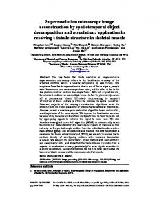
TABLE I: PSNR(dB)/SSIM results on the reconstructed HR images obtained by the NCSR method with different interpolations applied to the ‘Butterfly’ image for different scaling ratios. Ratios ×2 ×3

Oracle 31.32/0.9343 29.15/0.9270

SMSR1 30.50/0.9342 28.26/0.9192

Bicubic 30.33/0.9273 28.09/0.9160

Bilinear 30.32/0.9272 28.12/0.9164

Nearest 29.40/0.9206 27.22/0.8988

Fig. 1: Visual comparisons of the super-resolution results of the NCSR method with the different interpolations for the ‘Butterfly’ image (the scaling factor 3). From left to right: (a) Ground truth, (b) the oracle interpolation, (c) SMSR1, (d) the bicubic interpolation, (e) the bilinear interpolation, and (f) the nearest-neighbor interpolation.

begins with dictionary learning. Our dictionary learning adopts a multi-class and multi-level training framework, which is the same as that of the NCSR method [39]. Subsequently, according to the estimated image signal deviation, the reference histogram of gradients is estimated. After computing the transform function, the HR image is successively updated by the gradient histogram preservation regularization, the data fidelity constraint and the nonlocal means. After that, the HR image is sparsely coded over the trained dictionaries. Each element of the sparse coefficients is further updated with its nonlocal means by the shrinkage operator. The iteration proceeds until the convergence condition is reached. Finally, the target HR image xH is reconstructed by gathering the small image patches with the weighted averaging method. B. Gradual Magnification with Ridge Regression For only a LR image available for SR reconstruction, we need to build a training set of the LR and HR image pairs to restore the high-frequency details lost in the LR input. Since there is the self-similarity redundancy both within the same scale and across different scales, the input LR image and its degraded versions can be used to construct the LR and HR image pairs. Considering the different sizes of the LR and HR images, the LR input y is enlarged to the same size of the HR image x by the bicubic interpolation, whereas it is also a blurred and downsampled version of the HR image x. Therefore, the correspondence between the LR and HR images at the same scale is established as follows: z = (y) ↑ s = ((x ∗ G) ↓ s) ↑ s = Es x,

(4)

where ∗ is a convolution operator, ↑ s is an upsampling operator with the scaling factor s, ↓ s is a downsampling operator with the scaling factor s, G is a blurring kernel ( e.g., an isotropic Gaussian kernel with the standard deviation σG ), Es is a composite operator of blurring, downsampling and then upsampling with the scaling factor s, y is the LR image, x is the HR image, and z is the LR image at the same size of x. Note that the LR image is more similar to its HR image when the scaling factor is smaller, whereas the high-frequency

details tend to be lost when the scaling factor is larger. Therefore, in our example learning-based SR framework, we adopt the multi-step magnification scheme with the ridge regression for the initial estimation of the target HR image. For an input LR image y with a total scaling factor d, M = ⌈log (d) / log (s)⌉ is determined as the number of magnification steps, where s is the upscaling factor of each step. Specifically, the relationship between the HR image xsm at the m-th scale and the HR image xsm+1 at the (m + 1)-th scale can be expressed as follows: xsm = (xsm+1 ∗ Gs ) ↓ s.

(5)

And Eq. (4) in the multi-scale case can be written in another form: zsm = ((xsm ∗ Gs ) ↓ s) ↑ s = Es xsm , (6) where the input LR image y is regarded as the HR image xs0 at the scale m = 0. Specifically, the HR image xs0 is blurred and downsampled to generate the HR image xsm at the scale m = −1, · · · , −N . The LR image zs0 is produced by first downsampling the HR image xs0 and then upsampling the downsampled result by the bicubic interpolation. In our multi-step magnification scheme, we build two training sets: the LR image database Dz and the HR image database Dx . Specifically, the HR image xs0 is blurred and downsampled to produce the HR image xsm at the scale m = −1, · · · , −N . The HR image database Dx is constructed by collecting of these HR images xsm with the scale m = −1, · · · , −N . Correspondingly, the LR image zs0 is produced by first downsampling the HR image xs0 and then upsampling the downsampled result by the bicubic interpolation. Like the generation of the LR image zs0 , the LR image zsm at the scale m = −1, · · · , −N is also obtained by first downsampling the HR image xsm and then upsampling the downsampled result by the bicubic interpolation. The collection of these LR images zsm with the scale m = −1, · · · , −N is used to construct the LR image database Dz . Initially, the image databases Dz and Dx consist of all the patches of the LR image zsm and the HR image xsm at the scale m = 0, · · · , −N , respectively. At each step of the multi-step magnification process, for the

ZHANG et al.: IMAGE SUPER-RESOLUTION BASED ON STRUCTURE-MODULATED SPARSE REPRESENTATION

5

Fig. 2: Overview of the proposed SMSR method. The subgraphs with the solid boxes denote the specific techniques. The subgraph with the dashed box is the algorithm modules: gradual magnification, and sparse representation. upscaling ratio sm with m = 1, · · · , M , Dz and Dx are separately constructed by gathering the LR images zsn and the HR images xsn , where n = m − 1, · · · , −N . First, the LR image zsm is estimated from the HR image xsm−1 by the bicubic interpolation. For each patch yzi of the LR image zsm at the m-th scale, the ANN method is used to find the kn similar patches Nknl in the LR database Dz . We adopt the ridge regression to model the near-linear relationships between yzi and Nknl as the constrained optimization problem:

2 min yzi − Nknl γ 2 + τ ∥γ∥2 , (7) γ

where γ is the coefficient vector, and τ is a regularization parameter that alleviates the singularity problems and stabilizes the solution. By solving this regularized least squares regression problem, the closed-form solution is given by ( )−1 γ = NTknl Nknl + τ I NTknl yzi , (8) where I is an identity matrix. Then through transferring the mapping relationship from the LR space to the HR space, the HR patch can be reconstructed by multiplying the same coefficient vector and the corresponding HR patches as follows: yxi = Nknh γ,

(9)

where yxi is the corresponding HR patch of the HR image xsm at the m-th scale, and Nknh denotes the kn similar HR patches in the HR image database Dx . Next we compute all the HR patches yxi and then reconstruct the HR image xsm by the

weighted averaging method. The LR image zsm and the HR image xsm are separately added to the databases Dz and Dx . Subsequently, the multi-step magnification scheme proceeds to the next step, which enlarges xsm to xsm+1 . Finally, after the M steps of magnification, the HR image xsM is obtained for subsequent processing procedures. C. Structured Sparse Representation 1) SR Model: Since the HR image xsM reconstructed by the multi-step magnification scheme may be larger than the target HR image, the degraded version x0H of the right size is obtained by first blurring and then downsampling xsM with the bicubic interpolation. We use x0H as the initial value of the target HR image for sparse modeling of SR problem. Meanwhile, image gradients conveying abundant semantic features are crucial to the subjective visual image quality. Therefore, the histogram of image gradients can be used as a feature descriptor to constrain new image SR model. Besides that the gradual magnification is used as a preprocessing process for structured sparse representation, we propose the gradient histogram preservation regularization for single image SR modeling. That is, the gradient histogram of the reconstructed HR image should be close to that of the original HR image, which is estimated from the given LR image. Fig. 3 shows the flowchart of the proposed sparse representation of image SR model. Mathematically, our proposed structured sparse coding model of single image SR with multiple image priors is given

6

IEEE TRANSACTIONS ON IMAGE PROCESSING, VOL. XX, NO. XX, XX XXXX

LR input y available, we use the gradient histogram of y to infer that of the original HR image x. Different from the GHP for image denoising [34], we have extended the GHP regularization and provided the theoretical deduction for image super-resolution as follows. Let z denote the upsampled version of the LR image y that has the same size as the HR image x. For the observation model of image SR problem, Eq.(1) can be simply rewritten in the following formula: z = B ∗ x,

(13)

where B is a blurring operator. Thus we have ∑ ∇z = B ∗ ∇x = b0 ∇x + bi ∇xi ,

(14)

i

Fig. 3: The flowchart of our sparse representation of single image SR model.

as follows:

  2   ∥y − HΦ ◦ α∥2     ∑ ∥αi − βi ∥1 αy = arg min +λ1 , i  Φ,α,f     2 +λ2 ∥f (∇x|∇y) − ∇x∥

s.t.

(10)

hf = hr ,

where λ1 and λ2 are the regularization parameters, αi is the coding coefficients of each patch xi over the dictionary Φ, α denotes the concatenation of all αi , βi is the nonlocal means of αi in the sparse coding domain, ∇ denotes the gradient operator, f is the transform function, hr is the reference histogram of x, and hf is the histogram of the transformed gradient image |f (∇x|∇y)|. Note that f is an odd function that is monotonically non-descending in the domain (0, +∞). On the right side of (10), the first term is the data fidelity of the solution, the second term is the sparse nonlocal regularization [39] and the third term is our proposed gradient regularization. Considering the natural images usually contain repetitive patterns [36], the nonlocal similar patches to the given patch xi centered at pixel i are searched not only in the image spatial domain but also across different scales [10]. For the current estimate x ˆ, the similar patches of x ˆi are denoted by x ˆℓi , whose coding coefficients are αiℓ . Then βi can be computed as the weighted average of the sparse codes of the associated nonlocal similar patches [39]: ∑ βi = wiℓ αiℓ , (11)

where b0 and bi denotes the center coefficient and its surrounding neighbors of the blur kernel B, respectively. Assume that each pixel in the gradient image ∇x can be regarded as the value of a scalar random variable. The normalized histogram of ∇x is seen as a discrete approximation of the probability density function (PDF) of the random variable x. Since the PDF of x can be well modeled by a generalized Gaussian distribution [58], the assumption holds for the distribution of the gradient image ∇x. According to the Lyapunov central limit theorem in probability theory, the sum of independent ∑ random variables, i.e., i bi ∇xi , can be approximated by the normal ∑ distribution. Fig. 4 gives the real histogram distribution of i bi ∇xi for one example and the fitted PDF distribution of the random Gaussian variable g. The fitted PDF of the random Gaussian ∑variable g is very close to the real histogram distribution of i bi ∇xi with 95% confidence bounds. The experiments verify that both the theoretical deduction of our SMSR model and these assumptions are correct and hold in most cases. Then Eq. (14) can be reformulated in another form: z ≈ x + g,

(15) ) where g is a random Gaussian variable subject to N 0, σg2 , and z denotes a random variable for the distribution of the pixels in the gradient image ∇z. (

ℓ

where the weight

wiℓ

is defined as (

2 ) 1 exp − x ˆi − x ˆℓi 2 /h , (12) wiℓ = W where h is a control parameter to adjust ∑the decay rate and W is a normalized factor to insure that i wiℓ = 1. 2) Reference Histogram of Gradients: To solve the sparse coding problem in (10), we first need to know the reference histogram of gradients that is assumed to be the gradient histogram of the original HR image x. As there is only one

(a)

(b)

∑ Fig. 4: One example and the gradient histogram of i bi ∇xi . (a) Test image, (b) the comparison between the real histogram and the fitted PDF for the test image. In our algorithm, the one dimensional deconvolution model is built to estimate the reference histogram of gradients hr . Let hg be a discrete version of the PDF of a random Gaussian variable g. In fact, the standard deviation σg is unknown in

ZHANG et al.: IMAGE SUPER-RESOLUTION BASED ON STRUCTURE-MODULATED SPARSE REPRESENTATION

many image processing applications. To solve this problem, we use the signal variance of the input LR image y to estimate the distribution of g. According to Eq. (15), the reference histogram of gradients can be estimated by solving the deconvolution problem as follows: { } 2 hr = arg min ∥hz − hx ⊗ hg ∥ , (16) hx

where hz is the gradient histogram of the upsampled version of the LR input y, hx is the discrete version of the PDF of x that can be well modeled by a generalized Gaussian distribution [58], and hg is the discrete version of the PDF of the independent and identically distributed (i.i.d.) random variable g. 3) Numerical Solution: The mentioned above problem of image super-resolution is non-convex and is hard to solve exactly in a reasonable time. In our algorithm, we propose an alternating minimization method to solve the image SR problem in (10) so that the constrained optimization is carried out with some variables fixed in cyclical fashion. First, the multi-step magnification scheme is used to enlarge the input LR image y to get the HR image xsM at the M -th scale. Then the initial value of the target HR image is acquired by downsampling xsM with the bicubic interpolation method. Next, the iterative solution process starts with dictionary learning like that of the NCSR method [39]. Specifically, for the current estimation of HR image x, the k-means clustering is used to separate the patches of its multi-scale images into K clusters from each of which a sub-dictionary is trained by the principal component analysis (PCA). Subsequently, for each patch of the HR image, the PCA sub-dictionary of which cluster it belongs to is automatically selected as the dictionary Φ. For the fixed αi , βi and Φ, the image SR problem in (10) is reduced to the sub-problem of the GHP as follows: 2

min∥f (∇x|∇y) − ∇x∥ , f

s.t.

hf = hr .

(17)

Thus we can update the transform function f by solving the reduced sub-problem in (17). After that, for the fixed Φ and f , the image SR problem in (10) is reduced to the sub-problem in the following form: ∑ { } 2 ∥y − HΦ ◦ α∥2 + λ1 ∥αi − βi ∥1 i arg min , (18) 2 α +λ2 ∥f (∇x|∇y) − ∇x∥ where the parameter λ1 is used to weight the l1 -norm sparsity regularization term. Candes et al. [59] pointed out that iteratively reweighting the l1 -norm sparsity regularization term can lead to a better sparse representation. To improve the reconstruction of sparse signals, we adopt an adaptively reweighting method in [39], [41], [59] that exploits the image nonlocal redundancy to estimate the regularization parameter λ1 . To solve the convex minimization sub-problem in (18), we first update the HR image x by the gradient descent method as follows: ) (   x(t) HT y − Hˆ ) , ( (19) x ˆ(t+1/2) = x ˆ(t) + δ  (t) T x +λ2 ∇ f − ∇ˆ

7

where δ is a small constant. The update process of HR image in (19) can be divided into two stages: the gradient regularization and the data fidelity constraint. Therefore, the sparse coding coefficients αi are updated as follows: (t+1/2)

αi

= ΦTk Ri x ˆ(t+1/2) ,

(20)

where Φk , k = 1, · · · , K is the PCA sub-dictionary of a cluster that the patch x ˆi belongs to. The nonlocal means βi of αi can be estimated by Eq. (11). By employing the iterative shrinkage operator [50] applied to each element of αi , we can further update the coding coefficients αi in the following form:  ( )  (t+1/2) ΦT ◦ HT y − HΦ ◦ αi /c (t+1)  + βi , αi = Sλ/c  (t+1/2) +αi − βi (21) where Sλ/c is the soft thresholding function, and c is a regulatory parameter to ensure the convexity of the shrinkage function. Finally, the whole HR image is reconstructed as: x ˆ(t+1) = Φ(t+1) ◦ α(t+1) (∑ )−1 ∑ l l T = Ri Ri i=1

i=1

(

(t+1) (t+1) αi

RTi Φk

) .

(22)

Note that our proposed image SR model in (10) is similar in mathematical form to the one discussed by Attouch et al. [60], [61]. They proved that the minimization of the nonsmooth nonconvex objective function in the form of (10) can reach an abstract convergence result with descent methods under certain conditions. These conditions satisfy a sufficientdecrease assumption and allow a relative error tolerance. The above iterative procedures are executed repeatedly until the convergence condition is achieved [60], [61]. The theoretical convergence analysis of the proposed algorithm is left for our future research. More specifically, we select a certain number of iterations or a preset error tolerance as the convergence conditions of our algorithm for the simplicity. D. Method Summary To give further clarification of the specific implementation of our proposed SMSR algorithm, it is summarized in Algorithm 1. IV. E XPERIMENTAL R ESULTS In this work, numerous experimental studies on image super-resolution were carried out to verify the performance of our proposed SMSR algorithm. In our experiments, the basic parameters of our SMSR algorithm are set as follows: the patch size is 6 × 6 with the overlap width equal to 4 between the adjacent patches, K = 64, λ2 = 0.1, δ = 7, ε = 0.3, c = 0.35, s = 1.25, and τ = 0.1. Two cases of magnification ratios d = 2 and d = 3 were separately implemented for the test images. For d = 2, T1 = 7, T2 = 40 and M = 4, whereas for d = 3, T1 = 6, T2 = 160 and M = 5. The proposed SMSR algorithm was also compared with the bicubic interpolation method and the state-of-theart methods published recently [39], [41] for verifying its validity both subjectively and objectively. Indeed, our SMSR

8

IEEE TRANSACTIONS ON IMAGE PROCESSING, VOL. XX, NO. XX, XX XXXX

Algorithm 1 Pseudocodes of the SMSR-Based Image SuperResolution Input: a LR image y and a total scaling factor d. Output: a HR image xH . I. Initialization • Set the initial parameters λ1 , λ2 , δ and c; • Through exploiting the multi-scale similarity redundancy, the input LR image y is enlarged to obtain xsM by the multi-step magnification scheme; • Set the initial value of the target HR image that is d times the size of y by dowmsampling the enlarged result xsM ; II. Outer loop (dictionary learning and sparse coding): for each iteration t = 1 to T1 do • Update the dictionaries {Φk } by means of k-means clustering and PCA; • Compute the transform function f with the reference gradient histogram hr , and update the HR image x ˆ(t) by the gradient regularization; • Inner loop: for each iteration j = 1 to T2 do 1) Update x ˆ(t+1/2) by the fidelity constraint; 2) Compute the sparse coding coefficients of each (t+1/2) patch αi = ΦTk Ri x ˆ(t+1/2) , where Φk is the dictionary assigned to the patch x ˆi = Ri x ˆ(t+1/2) ; 3) Compute the regularization parameter λ1 and the (t+1/2) nonlocal means βi of αi ; (t+1) again by the 4) Update the coding coefficients αi iterative shrinkage operator using (21); 5) Reconstruct the estimate x ˆ(t+1) using (22); • Update the HR image xH = x ˆ(t+1) .

upscaling factor. To assess the impact of the patch size in the first stage, we have evaluated our SMSR1 with various size of image patch in the experiments. For the test ’Butterfly’ image, the PSNR(dB)/SSIM results are shown in Fig. 5 (a) and (b), where our SMSR1 achieves the best performance with the patch size of 5 × 5 for the total upscaling factor 2 and with the patch size of 7 × 7 for the total upscaling factor 3, respectively. Considering the balance between the computational complexity and the performance, the patch size is selected as 5 × 5 pixels in the first stage. Furthermore, we have assessed various size of image patch in the second stage of our SMSR algorithm. For the test ’Butterfly’ image, the PSNR(dB)/SSIM results are shown in Fig. 5 (c) and (d), where our SMSR2 achieves the best performance with the patch size of 5 × 5 pixels for both the total upscaling factors 2 and 3. Considering that the patch size is 6 × 6 pixels in the NCSR method [39], the patch size is also chosen as 6 × 6 pixels in the second stage of our SMSR algorithm for a fair comparison in the experiments. To assess the impact of the first stage in our SMSR framework, we have tested the different initialization methods. These initialization methods include the nearest interpolation, the bilinear interpolation, the bicubic interpolation, our proposed SMSR1 and the oracle interpolation method. The compared results of one example for objective and subjective evaluations are shown in Table II and Fig. 6, respectively. As can be seen from the results, our SMSR1 for the initial estimation of the target HR image is better than current competing interpolation methods and is very close to the performance of the oracle interpolation. The proposed SMSR algorithm and the current competing methods were separately applied to a set of test images from standard image databases. To evaluate the objective quality of the restored HR images, the PSNR and SSIM [62] were calculated for the comparisons of our SMSR algorithm and the state-of-the-art methods. For a fair comparison, we have implemented the qualitative and quantitative evaluation on the reconstructed HR images obtained by our proposed SMSR algorithm, the bicubic interpolation method, ANR [46], ASDS [41] and NCSR [39]. Considering the inter-scale similarity, the gradual magnification scheme instead of the interpolation method is used for the initial estimation of the target HR image in our SMSR model. For convenience, let SMSR ISS denote the united framework of NCSR [39] with the initialization by our multi-step gradual magnification scheme, and let SMSR GHP denote the GHP regularization combined with NCSR [39]. Both SMSR ISS and SMSR GHP have been separately implemented and compared with the current competing methods to evaluate the impact of the first stage and the GHP regularization of our SMSR model. Note that the bicubic interpolation is used for the initial estimation of the target HR image in the SMSR GHP model, whereas SMSR1 is used for the initial estimation of the target HR image in our SMSR model. For the set of test images, the PSNR/SSIM results of these different methods are shown in Table III for the total scaling factor d = 2 and Table IV for the total scaling factor d = 3, respectively. Both Table I and Fig. 1 show that the bicubic interpolation with the NCSR method

algorithm consists of two stages: the gradual magnification and the structured sparse representation (See Fig. 2). In this paper, for the convenience of our description, we refer to these two output stages as ‘SMSR1’ and ‘SMSR2’, respectively, where the output result of ‘SMSR2’ is also the final output of our proposed SMSR algorithm. Note that both the ScSR method [11] and the ANR method [46] adopt the bicubic interpolation for the generation of the simulated LR images in their reported experimental results. However, for a fair comparision, just like the other SR methods [39], [41], the Gaussian blurring and downsampling operator has been used to generate the simulated LR images in our experiments. That is, a HR image is first blurred with a 7 × 7 Gaussian kernel with standard deviation 1.6 and then downsampled by a total scaling factor d in both horizontal and vertical directions. Therefore, for test images, the simulated LR images in our experiments are different from those obtained by the bicubic interpolation in the experimental reports [11], [46]. For the color images, since the human visual system presents more sensitivity to the luminance changes, the image SR methods are only applied to the luminance component, whereas the chromatic components are zoomed in by the simple bicubic interpolation method. In our SMSR model, we have also researched on the patch size as a function of the

ZHANG et al.: IMAGE SUPER-RESOLUTION BASED ON STRUCTURE-MODULATED SPARSE REPRESENTATION

9

Fig. 5: The PSNR(dB)/SSIM results as a function of the patch size in the case of the different upscaling factors for the ‘Butterfly’ image. From left to right and top to bottom: (a) PSNR(dB) results of our SMSR1, (b) SSIM results of our SMSR1, (c) PSNR(dB) results of SMSR2 and (d) SSIM results of SMSR2. TABLE II: PSNR(dB)/SSIM results on the reconstructed HR images obtained by our SMSR framework with different interpolations applied to the ‘Butterfly’ image for different scaling ratios. Ratios ×2 ×3

Oracle 31.62/0.9367 29.39/0.9300

SMSR1 30.96/0.9464 28.48/0.9251

Bicubic 30.57/0.9295 28.29/0.9194

Bilinear 30.54/0.9295 28.26/0.9188

Nearest 28.04/0.9084 26.91/0.8950

Fig. 6: Visual comparisons of the super-resolution results of our SMSR framework with the different interpolations for the ‘Butterfly’ image (the total scaling factor 3). From left to right: (a) Ground truth, (b) the oracle interpolation, (c) SMSR1, (d) the bicubic interpolation, (e) the bilinear interpolation, and (f) the nearest-neighbor interpolation.

is usually superior to the nearest-neighbor interpolation or the bilinear interpolation with the NCSR method. Thus only the bicubic interpolation with the NCSR method is compared with our SMSR algorithm for performance evaluation. As can be seen from Table III to Table IV, it is found that the average PSNR gains of our SMSR algorithm over the second best method, i.e., NCSR [39], are about 0.4dB and 0.2dB for these test LR images, respectively. Moreover, for a comparison of the initialization of NCSR [39] and our SMSR algorithm, the average PSNR gains of our SMSR1 algorithm over the bicubic interpolation method are separately about 0.5dB and 0.2dB in the cases of d = 2 and d = 3. From the PSNR/SSIM results, our proposed SMSR algorithm is generally superior to the current state-of-the-art methods. To further inspect the effectiveness of our SMSR algorithm, the detailed reconstructed HR results of our SMSR algorithm and other competing methods [39], [41] for the test images are shown in Fig. 7 for the case d = 2 and Fig. 8 for the case d = 3, respectively. The visual comparisons between our SMSR algorithm and the baseline methods [39], [41] demonstrate that the proposed SMSR algorithm can recover finer structures and sharper edges and also has less color distortion for color image super-resolution. It is also found that our proposed SMSR algorithm has achieved noticeable performance gains in great part due to the knowledge of the blur kernel. Unlike Timofte et al. [46] and followers assuming sharp input LR images, the proposed

SMSR algorithm assumes that the blur kernel is known beforehand. As the initialization of our SMSR model, the example-based SMSR1 can achieve better results, especially for sharp input LR images, whereas our SMSR2 reaches its best performance with accurate blur kernel for image superresolution, which is especially useful when the input image is severely blurred. To the best of our knowledge, our proposed SMSR algorithm obviously outperforms the best existing stateof-the-art methods, e.g., NCSR [39], not only in the objective assessment but also in the visual comparisons. As seen from the experimental results, the proposed SMSR algorithm works well for a wide variety of images, and can reach better super-resolution results than the state-of-the-art methods both subjectively and objectively. V. C ONCLUSIONS AND F UTURE W ORK In this paper, we proposed a solution to the single image super-resolution problem with an SMSR method. Since there is abundant similarity redundancy both within the same scale and across the different scales, the multi-scale magnification scheme with the ridge regression is first used to compute the initial estimation of the target HR image. Then the sparse modeling of single image super-resolution is designed with a gradient regularization term that preserves the gradient histogram of the target HR image. Another centralized sparse constraint that exploits the image local and nonlocal redundancy is also

10

IEEE TRANSACTIONS ON IMAGE PROCESSING, VOL. XX, NO. XX, XX XXXX

Fig. 7: Visual comparisons of the super-resolution results of the proposed SMSR algorithm and other state-of-the-art methods for test images (the total scaling factor 2). These test images include ‘Brain’, ‘Butterfly’, ‘Comic’ and ‘Hat’. From left to right and top to bottom: (a) LR input, (b) ground truth, (c) our SMSR2, (d) NCSR [39], (e) ASDS [41], (f) the bicubic interpolation, (g) ANR [46], (h) our SMSR1, (i) our SMSR ISS and (j) our SMSR GHP. Zoom into pdf file for a detailed view.

ZHANG et al.: IMAGE SUPER-RESOLUTION BASED ON STRUCTURE-MODULATED SPARSE REPRESENTATION

11

Fig. 8: Visual comparisons of the super-resolution results of the proposed SMSR algorithm and other state-of-the-art methods for test images (the total scaling factor 3). These test images include ‘Brain’, ‘Butterfly’, ‘Comic’ and ‘Hat’. From left to right and top to bottom: (a) LR input, (b) ground truth, (c) our SMSR2, (d) NCSR [39], (e) ASDS [41], (f) the bicubic interpolation, (g) ANR [46], (h) our SMSR1, (i) our SMSR ISS and (j) our SMSR GHP. Zoom into pdf file for a detailed view.

12

IEEE TRANSACTIONS ON IMAGE PROCESSING, VOL. XX, NO. XX, XX XXXX

TABLE III: PSNR(dB)/SSIM results on the reconstructed HR images with the total scaling factor d = 2. Images Bike Brain Butterfly Comic Flower Hat Leaves Parrot Parthenon Plants Raccoon SunFlower Average

SMSR2 27.34/0.8820 31.69/0.8931 30.96/0.9464 27.39/0.8844 31.75/0.9075 33.39/0.9049 31.56/0.9639 32.86/0.9335 28.93/0.8217 36.23/0.9409 31.24/0.8552 30.53/0.8997 31.16/0.9028

NCSR [39] 27.17/0.8729 31.52/0.8970 30.33/0.9273 27.34/0.8775 31.52/0.8925 32.74/0.8755 30.85/0.9511 32.37/0.9045 28.73/0.8079 35.35/0.9172 31.12/0.8537 30.40/0.8931 30.79/0.8892

ASDS [41] 26.95/0.8722 30.78/0.8764 29.65/0.9371 27.10/0.8763 31.34/0.9008 32.94/0.9061 30.47/0.9552 32.25/0.9322 28.49/0.8058 35.68/0.9383 30.96/0.8450 30.31/0.8954 30.58/0.8951

Bicubic 21.90/0.6478 26.17/0.7289 22.42/0.7802 22.15/0.6415 26.25/0.7421 28.30/0.8081 21.62/0.7378 26.87/0.8588 25.26/0.6689 29.57/0.8353 27.50/0.6826 24.85/0.7233 25.24/0.7379

ANR [46] 22.19/0.6771 26.49/0.7480 22.80/0.8034 22.40/0.6707 26.41/0.7642 28.32/0.8215 21.87/0.7674 26.90/0.8697 25.45/0.6868 29.66/0.8503 27.59/0.7019 24.96/0.7456 25.42/0.7589

SMSR1 22.27/0.6774 26.63/0.7513 23.21/0.8195 22.48/0.6701 26.67/0.7672 28.85/0.8270 22.38/0.7903 27.42/0.8713 25.57/0.6885 30.04/0.8529 27.78/0.7018 25.20/0.7455 25.71/0.7636

SMSR ISS 27.29/0.8738 31.75/0.8978 30.50/0.9342 27.34/0.8774 31.56/0.8990 33.02/0.8935 31.04/0.9569 32.56/0.9188 28.82/0.8179 35.54/0.9243 31.06/0.8509 30.29/0.8890 30.90/0.8944

SMSR GHP 27.26/0.8751 31.60/0.8977 30.57/0.9295 27.38/0.8788 31.58/0.8933 32.81/0.8763 31.05/0.9528 32.45/0.9048 28.77/0.8088 35.41/0.9176 31.15/0.8538 30.44/0.8938 30.87/0.8902

TABLE IV: PSNR(dB)/SSIM results on the reconstructed HR images with the total scaling factor d = 3. Images Bike Brain Butterfly Comic Flower Hat Leaves Parrot Parthenon Plants Raccoon SunFlower Average

SMSR2 24.95/0.8107 29.56/0.8434 28.48/0.9251 24.72/0.7950 29.68/0.8618 31.60/0.8768 27.77/0.9302 30.76/0.9186 27.24/0.7550 34.23/0.9211 29.33/0.7717 28.05/0.8405 28.86/0.8542

NCSR [39] 24.72/0.8026 29.36/0.8407 28.09/0.9160 24.65/0.7909 29.51/0.8567 31.26/0.8701 27.46/0.9217 30.53/0.9148 27.18/0.7508 34.03/0.9189 29.28/0.7711 27.93/0.8377 28.67/0.8494

ASDS [41] 24.60/0.7959 28.81/0.8251 27.30/0.9049 24.48/0.7819 29.17/0.8463 30.99/0.8714 26.94/0.9101 30.09/0.9101 26.89/0.7369 33.41/0.9072 29.23/0.7655 27.89/0.8331 28.32/0.8407

Bicubic 20.80/0.5759 24.75/0.6660 20.78/0.7175 20.87/0.5573 24.83/0.6753 27.20/0.7778 19.83/0.6411 25.58/0.8261 24.12/0.6205 27.83/0.7875 26.38/0.6280 23.22/0.6466 23.85/0.6766

incorporated to improve the performance of the image sparse representation. To approximate the global optimization result, which is nonconvex and hard to solve directly, an alternating minimization method with an iteratively reweighted regularization parameter is used to solve the structure-constrained optimization problem of single image super-resolution. The sparse coefficients of the estimated HR image are further corrected by an efficient iterative shrinkage function. We have conducted extensive experiments on image super-resolution and evaluated the results of both the proposed algorithm and the popular SR methods. Experimental results demonstrated that our SMSR algorithm that can produce sharper edges and suppress aliasing artifacts is promising and competitive to the state-of-the-art methods, and outperforms other leading SR methods both visually and quantitatively in most cases. To further improve the performance and the efficiency of superresolution, we will study on accurate estimation of blur kernel and noisy image super-resolution in the future.

[6] [7] [8]

[9] [10] [11] [12] [13]

R EFERENCES [14] [1] P. Milanfar, Ed., Super-resolution imaging (digital imaging and computer vision). New York: CRC Press, Sep. 21, 2010. [2] R. Y. Tsai and T. S. Huang, Multipleframe image restoration and registration, ser. In Advances in Computer Vision and Image Processing. Greenwich, Conn, USA: JAI Press Inc., 1984, vol. 1. [3] W. C. Siu and K. W. Hung, “Review of image interpolation and superresolution,” Asia-Pacific Signal and Information Processing Association Annual Summit and Conference, p. 10, 2012. [4] M. Irani and S. Peleg, “Improving resolution by image registration,” CVGIP-Graphical Models and Image Processing, vol. 53, no. 3, pp. 231–239, 1991. [5] R. C. Hardie, K. J. Barnard, and E. E. Armstrong, “Joint map registration and high-resolution image estimation using a sequence of undersampled

[15]

[16] [17]

ANR [46] 21.11/0.6170 24.95/0.6892 21.19/0.7567 21.03/0.5930 24.98/0.7051 27.27/0.7951 20.05/0.6841 25.84/0.8414 24.25/0.6392 27.91/0.8061 26.24/0.6453 23.25/0.6711 24.00/0.7036

SMSR1 21.05/0.6148 24.84/0.6833 21.39/0.7723 21.04/0.5879 24.82/0.7021 27.51/0.7958 20.06/0.7039 26.19/0.8422 24.18/0.6320 27.92/0.8034 26.49/0.6452 23.42/0.6713 24.08/0.7045

SMSR ISS 24.77/0.8034 29.42/0.8415 28.26/0.9192 24.67/0.7912 29.59/0.8594 31.40/0.8738 27.69/0.9271 30.60/0.9170 27.21/0.7528 34.09/0.9202 29.28/0.7711 27.96/0.8380 28.74/0.8512

SMSR GHP 24.79/0.8054 29.43/0.8420 28.29/0.9193 24.68/0.7926 29.56/0.8578 31.37/0.8719 27.62/0.9252 30.56/0.9156 27.21/0.7521 34.15/0.9201 29.29/0.7710 27.98/0.8389 28.74/0.8510

images,” IEEE Transactions on Image Processing, vol. 6, no. 12, pp. 1621–1633, 1997. S. Farsiu, M. Elad, and P. Milanfar, “Video-to-video dynamic superresolution for grayscale and color sequences,” EURASIP Journal on Applied Signal Processing, p. 15, 2006. A. Marquina and S. J. Osher, “Image super-resolution by tvregularization and bregman iteration,” Journal of Scientific Computing, vol. 37, no. 3, pp. 367–382, 2008. X. Zhang, J. Jiang, and S. Peng, “Commutability of blur and affine warping in super-resolution with application to joint estimation of triplecoupled variables,” IEEE Transactions on Image Processing, vol. 21, no. 4, pp. 1796–1808, 2012. W. T. Freeman, T. R. Jones, and E. C. Pasztor, “Example-based superresolution,” IEEE Computer Graphics and Applications, vol. 22, no. 2, pp. 56–65, 2002. D. Glasner, S. Bagon, and M. Irani, “Super-resolution from a single image,” in Proceedings of IEEE International Conference on Computer Vision, 2009, pp. 349–356. J. C. Yang, J. Wright, T. S. Huang, and Y. Ma, “Image super-resolution via sparse representation,” IEEE Transactions on Image Processing, vol. 19, no. 11, pp. 2861–2873, 2010. K. I. Kim and Y. Kwon, “Single-image super-resolution using sparse regression and natural image prior,” IEEE Transactions on Pattern Analysis and Machine Intelligence, vol. 32, no. 6, pp. 1127–1133, 2010. J. Sun, Z. B. Xu, and H. Y. Shum, “Gradient profile prior and its applications in image super-resolution and enhancement,” IEEE Transactions on Image Processing, vol. 20, no. 6, pp. 1529–1542, 2011. X. B. Gao, K. B. Zhang, D. C. Tao, and X. L. Li, “Joint learning for single-image super-resolution via a coupled constraint,” IEEE Transactions on Image Processing, vol. 21, no. 2, pp. 469–480, 2012. S. P. Kim, N. K. Bose, and H. M. Valenzuela, “Recursive reconstruction of high-resolution image from noisy undersampled multiframes,” IEEE Transactions on Acoustics Speech and Signal Processing, vol. 38, no. 6, pp. 1013–1027, 1990. H. Ur and D. Gross, “Improved resolution from subpixel shifted pictures,” CVGIP-Graphical Models and Image Processing, vol. 54, no. 2, pp. 181–186, 1992. M. S. Alam, J. G. Bognar, R. C. Hardie, and B. J. Yasuda, “Infrared image registration and high-resolution reconstruction using multiple translationally shifted aliased video frames,” IEEE Transactions on Instrumentation and Measurement, vol. 49, no. 5, pp. 915–923, 2000.

ZHANG et al.: IMAGE SUPER-RESOLUTION BASED ON STRUCTURE-MODULATED SPARSE REPRESENTATION

[18] H. Takeda, S. Farsiu, and P. Milanfar, “Kernel regression for image processing and reconstruction,” IEEE Transactions on Image Processing, vol. 16, no. 2, pp. 349–366, 2007. [19] M. Elad and A. Feuer, “Restoration of a single superresolution image from several blurred, noisy, and undersampled measured images,” IEEE Transactions on Image Processing, vol. 6, no. 12, pp. 1646–1658, 1997. [20] D. Capel and A. Zisserman, “Computer vision applied to super resolution,” IEEE Signal Processing Magazine, vol. 20, no. 3, pp. 75–86, 2003. [21] L. C. Pickup, D. P. Capel, S. J. Roberts, and A. Zisserman, “Bayesian methods for image super-resolution,” Computer Journal, vol. 52, no. 1, pp. 101–113, 2009. [22] L. J. Karam, N. G. Sadaka, R. Ferzli, and Z. A. Ivanovski, “An efficient selective perceptual-based super-resolution estimator,” IEEE Transactions on Image Processing, vol. 20, no. 12, pp. 3470–3482, 2011. [23] H. Stark and P. Oskoui, “High-resolution image recovery from imageplane arrays, using convex projections,” Journal of the Optical Society of America A-Optics Image Science and Vision, vol. 6, no. 11, pp. 1715– 1726, 1989. [24] X. H. Zhang, M. Tang, and R. F. Tong, “Robust super resolution of compressed video,” Visual Computer, vol. 28, no. 12, pp. 1167–1180, 2012. [25] S. Izadpanahi and H. Demirel, “Motion based video super resolution using edge directed interpolation and complex wavelet transform,” Signal Processing, vol. 93, no. 7, pp. 2076–2086, 2013. [26] J. Salvador, A. Kochale, and S. Schweidler, “Patch-based spatiotemporal super-resolution for video with non-rigid motion,” Signal Processing-Image Communication, vol. 28, no. 5, pp. 483–493, 2013. [27] X. Li and M. T. Orchard, “New edge-directed interpolation,” IEEE Transactions on Image Processing, vol. 10, no. 10, pp. 1521–1527, 2001. [28] Z. Wei and K. K. Ma, “Contrast-guided image interpolation,” IEEE Transactions on Image Processing, vol. 22, no. 11, pp. 4271–4285, 2013. [29] K. Jia, X. G. Wang, and X. O. Tang, “Image transformation based on learning dictionaries across image spaces,” IEEE Transactions on Pattern Analysis and Machine Intelligence, vol. 35, no. 2, pp. 367–380, 2013. [30] S. Baker and T. Kanade, “Limits on super-resolution and how to break them,” IEEE Transactions on Pattern Analysis and Machine Intelligence, vol. 24, no. 9, pp. 1167–1183, 2002. [31] Z. C. Lin and H. Y. Shum, “Fundamental limits of reconstruction-based superresolution algorithms under local translation,” IEEE Transactions on Pattern Analysis and Machine Intelligence, vol. 26, no. 1, pp. 83–97, 2004. [32] L. I. Rudin, S. Osher, and E. Fatemi, “Nonlinear total variation based noise removal algorithms,” Physica D, vol. 60, no. 1-4, pp. 259–268, 1992. [33] R. Fergus, B. Singh, A. Hertzmann, S. T. Roweis, and W. T. Freeman, “Removing camera shake from a single photograph,” Acm Transactions on Graphics, vol. 25, no. 3, pp. 787–794, 2006. [34] W. M. Zuo, L. Zhang, C. W. Song, and D. Zhang, “Texture enhanced image denoising via gradient histogram preservation,” in Proceedings of IEEE Conference on Computer Vision and Pattern Recognition, 2013, pp. 1203–1210. [35] Y. Q. Zhang, J. Y. Liu, M. D. Li, and Z. M. Guo, “Joint image denoising using adaptive principal component analysis and self-similarity,” Information Sciences, vol. 259, pp. 128–141, 2014. [36] A. Buades, B. Coll, and J. M. Morel, “A review of image denoising algorithms, with a new one,” SIAM Multiscale Modeling and Simulation, vol. 4, no. 2, pp. 490–530, 2005. [37] V. Katkovnik, A. Foi, K. Egiazarian, and J. Astola, “From local kernel to nonlocal multiple-model image denoising,” International Journal of Computer Vision, vol. 86, no. 1, pp. 1–32, 2010. [38] J. Mairal, F. Bach, J. Ponce, G. Sapiro, and A. Zisserman, “Nonlocal sparse models for image restoration,” in Proceedings of IEEE International Conference on Computer Vision, 2009, pp. 2272–2279. [39] W. S. Dong, L. Zhang, G. M. Shi, and X. Li, “Nonlocally centralized sparse representation for image restoration,” IEEE Transactions on Image Processing, vol. 22, no. 4, pp. 1618–1628, 2013. [40] A. M. Bruckstein, D. L. Donoho, and M. Elad, “From sparse solutions of systems of equations to sparse modeling of signals and images,” SIAM Review, vol. 51, no. 1, pp. 34–81, 2009. [41] W. S. Dong, L. Zhang, G. M. Shi, and X. L. Wu, “Image deblurring and super-resolution by adaptive sparse domain selection and adaptive regularization,” IEEE Transactions on Image Processing, vol. 20, no. 7, pp. 1838–1857, 2011. [42] Y. Q. Zhang, Y. Ding, J. S. Xiao, J. Y. Liu, and Z. M. Guo, “Visibility enhancement using an image filtering approach,” EURASIP Journal on Advances in Signal Processing, p. 6, 2012.

13

[43] Y. Q. Zhang, Y. Ding, J. Y. Liu, and Z. M. Guo, “Guided image filtering using signal subspace projection,” IET Image Processing, vol. 7, no. 3, pp. 270–279, 2013. [44] C. Dong, C. C. Loy, K. He, and X. Tang, “Learning a deep convolutional network for image super-resolution,” in Proceedings of European Conference on Computer Vision (ECCV), vol. 8692, 2014, pp. 184–199. [45] T. Michaeli and M. Irani, “Nonparametric blind super-resolution,” in Proceedings of IEEE International Conference on Computer Vision, 2013, pp. 945 – 952. [46] R. Timofte, V. De, and L. Van Gool, “Anchored neighborhood regression for fast example-based super-resolution,” in Proceedings of IEEE International Conference on Computer Vision, 2013, pp. 1920–1927. [47] ——, “A+: adjusted anchored neighborhood regression for fast superresolution,” in Proceedings of Asian Conference on Computer Vision, 2014, pp. 1–15. [48] E. Perez-Pellitero, J. Salvador, I. Torres, J. Ruiz-Hidalgo, and B. Rosenhahn, “Fast super-resolution via dense local training and inverse regressor search,” in Proceedings of Asian Conference on Computer Vision, 2014, pp. 1–14. [49] H. A. Aly and E. Dubois, “Image up-sampling using total-variation regularization with a new observation model,” IEEE Transactions on Image Processing, vol. 14, no. 10, pp. 1647–1659, 2005. [50] I. Daubechies, M. Defrise, and C. De Mol, “An iterative thresholding algorithm for linear inverse problems with a sparsity constraint,” Communications on Pure and Applied Mathematics, vol. 57, no. 11, pp. 1413–1457, 2004. [51] J. A. Tropp and S. J. Wright, “Computational methods for sparse solution of linear inverse problems,” Proceedings of the IEEE, vol. 98, no. 6, pp. 948–958, 2010. [52] G. Peyre, S. Bougleux, and L. Cohen, “Non-local regularization of inverse problems,” Inverse Problems and Imaging, vol. 5, no. 2, pp. 511–530, 2011. [53] M. Aharon, M. Elad, and A. Bruckstein, “K-svd: an algorithm for designing overcomplete dictionaries for sparse representation,” IEEE Transactions on Signal Processing, vol. 54, no. 11, pp. 4311–4322, 2006. [54] J. Mairal, G. Sapiro, and M. Elad, “Learning multiscale sparse representations for image and video restoration,” SIAM Multiscale Modeling and Simulation, vol. 7, no. 1, pp. 214–241, 2008. [55] R. Rubinstein, M. Zibulevsky, and M. Elad, “Double sparsity: learning sparse dictionaries for sparse signal approximation,” IEEE Transactions on Signal Processing, vol. 58, no. 3, pp. 1553–1564, 2010. [56] J. Mairal, F. Bach, and J. Ponce, “Task-driven dictionary learning,” IEEE Transactions on Pattern Analysis and Machine Intelligence, vol. 34, no. 4, pp. 791–804, 2012. [57] Y. Q. Zhang, J. S. Xiao, S. H. Li, C. Y. Shi, and G. X. Xie, “Learning block-structured incoherent dictionaries for sparse representation,” Science China Information Sciences, vol. 58, pp. 102 302:1–15, 2015. [58] T. S. Cho, C. L. Zitnick, N. Joshi, S. B. Kang, R. Szeliski, and W. T. Freeman, “Image restoration by matching gradient distributions,” IEEE Transactions on Pattern Analysis and Machine Intelligence, vol. 34, no. 4, pp. 683–694, 2012. [59] E. J. Candes, M. B. Wakin, and S. P. Boyd, “Enhancing sparsity by reweighted l(1) minimization,” Journal of Fourier Analysis and Applications, vol. 14, no. 5-6, pp. 877–905, 2008. [60] H. Attouch, J. Bolte, P. Redont, and A. Soubeyran, “Proximal alternating minimization and projection methods for nonconvex problems: an approach based on the kurdyka-lojasiewicz inequality,” Mathematics of Operations Research, vol. 35, no. 2, pp. 438–457, 2010. [61] H. Attouch, J. Bolte, and B. F. Svaiter, “Convergence of descent methods for semi-algebraic and tame problems: proximal algorithms, forwardbackward splitting, and regularized gauss-seidel methods,” Mathematical Programming, vol. 137, no. 1-2, pp. 91–129, 2013. [62] Z. Wang, A. C. Bovik, H. R. Sheikh, and E. P. Simoncelli, “Image quality assessment: from error visibility to structural similarity,” IEEE Transactions on Image Processing, vol. 13, no. 4, pp. 600–612, 2004.

14

IEEE TRANSACTIONS ON IMAGE PROCESSING, VOL. XX, NO. XX, XX XXXX

Yongqin Zhang (M’13) received the B.S.E. degree in Electronics Science and Technology in 2005 from Zhengzhou University, P. R. China, and the Ph.D. degree in Communication and Information Systems in 2010 from Wuhan University, P. R. China, respectively. He is currently a postdoctoral researcher with the Institute of Computer Science and Technology, Peking University. His research interests include magnetic resonance imaging, sparse representation and image restoration.

Jiaying Liu (S’09-M’10) received the B.E. degree in computer science from Northwestern Polytechnic University, Xi’an, China, and the Ph.D. degree with the Best Graduate Honor in computer science from Peking University, Beijing, China, in 2005 and 2010, respectively. She was a Visiting Scholar with the University of Southern California, Los Angeles, from 2007 to 2008. She is currently an Associate Professor with the Institute of Computer Science and Technology, Peking University. Her current research interests include image processing, sparse signal representation, and video compression.

Wenhan Yang received the B.S degree in Computer Science from Peking University, Beijing, China, in 2008. He is currently a Ph.D. student with the Institute of Computer Science and Technology, Peking University. His current research interests include image processing, sparse representation and image restoration.

Zongming Guo (M’09) received the B.S. degree in mathematics, and the M.S. and Ph.D. degrees in computer science from Peking University, Beijing, China, in 1987, 1990, and 1994, respectively. He is currently a Professor with the Institute of Computer Science and Technology, Peking University. His current research interests include video coding, processing, and communication. Dr. Guo is the Executive Member of the China Society of Motion Picture and Television Engineers. He was a recipient of the First Prize of the State Administration of Radio Film and Television Award in 2004, the First Prize of the Ministry of Education Science and Technology Progress Award in 2006, the Second Prize of the National Science and Technology Award in 2007, the Wang Xuan News Technology Award and the Chia Tai Teaching Award in 2008, and the Government Allowance granted by the State Council in 2009.