To appear in Microcomputers in Civil Engineering: Special Issue on Active and Hybrid Structural Control
Implementation of an AMD Using Acceleration Feedback Control S.J. Dyke,1 B.F. Spencer Jr.,1 P. Quast,2 D.C. Kaspari, Jr.,1 and M.K. Sain2 Abstract Most of the current research on active structural control for aseismic protection has focused on either full state feedback strategies or velocity feedback strategies. However, accurate measurement of the necessary displacements and velocities of the structure is difficult to achieve directly, particularly during seismic activity. Because accelerometers are inexpensive and can readily provide reliable measurement of the structural accelerations at strategic points on the structure, development of control methods based on acceleration feedback is an ideal solution to this problem. Recent studies of active bracing and active tendon systems have shown that H 2 / LQG frequency domain control methods employing acceleration feedback can effectively be used for aseismic protection of structures. This paper demonstrates experimentally the efficacy of acceleration feedback based active mass driver systems in reducing the response of seismically excited structures. 1.0 Introduction A remarkable increase in structural control research has occurred in the last decade (cf., [15, 16, 29]). Most of the reported studies dealing with active and hybrid control have been based on methods employing full state feedback (i.e., the structural displacements and velocities) or velocity feedback. Because displacements and velocities are not absolute, but dependent upon the inertial reference frame in which they are taken, their direct measurement at arbitrary locations on large-scale structures is difficult to achieve. During seismic activity, this difficulty is exacerbated, because the foundation to which the structure is attached is moving with the ground and does not provide an inertial reference frame. Thus, control algorithms that are dependent on direct measurement of the displacements and velocities may be impracticable for full-scale implementations. Alternatively, accelerometers can provide inexpensive and reliable measurements of the accelerations at strategic points on the structure, making the use of absolute structural acceleration measurements for control force determination an ideal way to avoid this problem. Previous experiments have shown acceleration feedback strategies to be effective for both an active bracing system [31] and an active tendon system [5, 7]. The control algorithms used in those experiments were based on previous studies discussed in [30, 33]. This paper expands upon the experimental verification of acceleration feedback control strategies for active mass driver (AMD) systems reported in [6]. A three-story test structure equipped with an AMD system was employed in the research, which was conducted at the Structural Dynamics and Control/Earthquake Engineering Laboratory at the University of Notre Dame. Frequency domain H 2 /LQG optimal control strategies were employed to achieve the control objectives. Control-structure interaction models were incorporated into the analysis. The results indicate that AMD systems employing acceleration feedback strategies are effective for reduction of structural responses dur1. Department. of Civil Engrg. and Geolog. Sci., University of Notre Dame, IN, 46556. 2. Department of Electrical Engrg., University of Notre Dame, IN, 46556. 1
ing seismic activity and that response reduction can be achieved in all three modes of the structural system. 2.0 Experimental Setup Tests were conducted at the Structural Dynamics and Control/ Earthquake Engineering Laboratory (SDC/EEL) at the University of Notre Dame. A uniaxial earthquake simulator which was designed and built under National Science Foundation Grant BCS 90-06781 is housed in the laboratory. The simulator consists of a hydraulic actuator/servo-valve assembly that drives a 48in × 48in ( 122cm × 122cm ) aluminum slip table mounted on high-precision, low-friction, linear bearings. The capabilities of the simulator are: maximum displacement ± 2in ( ± 5.1 cm), maximum velocity ± 35 in/sec ( ± 88.9 cm/sec) and maximum acceleration ± 4 gs with a 1000 lb (454.5 kg) test load. The operational frequency range of the simulator is nominally 0–50 Hz. A three-story, single-bay, scale model building was the test structure. The test structure, shown in Figs. 1 and 2, was designed to be a scale model of the prototype building discussed in [4]. The building frame was constructed of steel, with a height of 62 in (157.5 cm). The floor masses of the model weighed a total of 500 lb (227 kg), distributed evenly between the three floors. The time scale factor was 0.2, making the natural frequencies of the model approximately five times those of the prototype. A simple implementation of an active mass driver (AMD) was placed on the third floor of the structure for control purposes. The AMD consisted of a high pressure hydraulic actuator with steel masses attached to each end of the piston rod (Fig. 3). The hydraulic cylinder, manufactured by Nopak, had a 1.5 in (3.8 cm) diameter and a 12 in (30.5 cm) stroke. A Dyval servo-valve was employed that had an operational frequency range of 0–45 Hz. This hydraulic actuator was fitted with low-friction Teflon seals to reduce nonlinear frictional effects. For this experiment, the moving mass for the AMD weighed 11.5 lb (5.2 kg) and consisted of the piston, piston rod and the steel disks bolted to the end of the piston rod. The total mass of the structure, including the frame and the AMD, was 660 lbs (300 kg). Thus, the moving mass of the AMD was 1.7% of the total mass of the structure. Because hydraulic actuators are inherently open loop unstable, position feedback was employed to stabilize the control actuator. The position of the actuator was obtained with an LVDT (linear variable differential transformer) rigidly mounted between the piston rod and the third floor. As shown in Fig. 2, accelerometers positioned on each floor of the structure and on the AMD measured the absolute accelerations of the model, and an accelerometer located on the base measured the ground excitation. The displacement of the AMD relative to the third floor was measured using the LVDT mentioned above. Only the three floor acceleration measurements and the absolute acceleration of the AMD were employed for purposes of control force determination (see Fig. 2). To develop a high quality, control-oriented model, Figure 1. Experimental Setup. an eight channel data acquisition system was em-
2
u ( t)
x˙˙aa ( t ) y ( t)
x˙˙a3 ( t )
DSP Board
x˙˙a2 ( t )
D/A x k + 1 = Ax k + By k u k = Cx k + Dy k Digital Control Algorithm
x˙˙a1 ( t ) Shaking Table
x˙˙g ( t )
A/D
Figure 2. Schematic of Experimental Setup.
ployed. This data acquisition system consists of eight Syminex XFM82 3-decade programmable antialiasing filters, an Analogic LSDAS-16-AC-mod2 data acquisition board, an Analogic CTRTM-05 counter-timer board, and the Snap-Master software package written by HEM Data Corporation, driven by a Gateway 2000 P5-90 Computer. The XFM82 series filters offer programmable pre-filter gains to amplify the signal into the filter, programmable post-filter gains to adjust the signal so that it falls in the correct range for the A/D converter, and analog antialiasing filters which are programmable up to 25 kHz. The highquality elliptic low-pass filter has a 0.001 dB pass-band ripple, a stop band magnitude of -90 dB, and a 90 dB/oct roll-off above the cutoff frequency. The filters on all 8-channels are magnitude/ phase matched to within 0.1 dB/1 degree to 90% of the cutoff frequency. In addition, each channel has a sample-and-hold device to allow simultaneous measurement of all signals. Simultaneous sample-and-hold (SSH) is necessary to eliminate systematic bias in the phase of the transfer functions. The Analogic LSDAS-16-AC-mod2 data acquisition board is a high speed, high precision multifunction board featuring 50 kHz sampling and 16 bits of A/D resolution. The LSDAS-16AC-mod2 can measure up to 8 channels in the differential input mode. This mode is recommended for noise rejection and resistance to ground loops. To take full advantage of the SSH ability of the XFM82 filters, the sample-and-hold and A/D conversion are triggered with an external clock source supplied by a CTRTM-05 counter-timer board which generates the appropriate timing signals. Snap-Master for Windows provides the necessary drivers for the antialiasing filters, countertimer board and data acquisition board. Snap-Master also has the required time and frequency domain functions which can be used to analyze the data during testing or post processing. Additionally, Snap-Master allows the user to create custom instruments. Implementation of the digital controller was performed using the Spectrum Signal Processing Real-Time Digital Signal Processor (DSP) System. It is configured on a board that plugs into a 16-bit slot in a PC’s expansion bus and features a Texas Instruments TMS320C30 Digital Signal
3
Processor chip, RAM memory and on board A/D and D/A systems. The TMS320C30 DSP chip can achieve a nominal performance of 16.7 MFLOPS. The onboard A/D system has two channels, each with 16 bit precision and a maximum sampling rate of 200 kHz. The two D/A channels, also with 16 bit precision, allow for even greater output rates so as not to be limiting. An expansion I/O daughter board provides an additional four channels of input and two channels of output. These input channels provide 12 bit precision Figure 3. Active mass driver. and have a maximum sampling rate of 50 kHz per channel. Thus, the computer controller employed herein can accommodate up to 6 inputs and 4 outputs. With the high computation rates of the DSP chip and the extremely fast sampling and output capability of the associated I/O system, high overall sampling rates are achievable for the digital control system [7, 26, 33]. 3.0 System Identification Development of an accurate mathematical model of the structural system is one of the most important and challenging components of control design. There are several methods by which to accomplish this task. One approach is to analytically derive the system input/output characteristics by physically modeling the plant. Often this technique results in complex models that do not correlate well with the observed response of the physical system. An alternative approach to developing the necessary dynamical model of the structural system is to measure the input/output relationships of the system and construct a mathematical model that can replicate this behavior. This approach is termed system identification in the control systems literature. The steps in this process are as follows: (i) collect high-quality input/output data (the quality of the model is tightly linked to the quality of the data on which it is based), (ii) compute the best model within the class of systems considered, and (iii) evaluate the adequacy of the model’s properties. For linear structures, system identification techniques fall into two categories: time domain and frequency domain. Time domain techniques such as the recursive least squares (RLS) system identification method [9] are superior when limited measurement time is available. Frequency domain techniques are generally preferred when significant noise is present in the measurements and the system is assumed to be linear and time invariant. In the frequency domain approach to system identification, the first step is to experimentally determine the transfer functions (also termed frequency response functions) from each of the system inputs to each of the outputs. Subsequently, each of the experimental transfer functions is modeled as a ratio of two polynomials in the Laplace variable s and then used to form a state space representation for the structural system. The frequency domain system identification approach will be employed herein for the development of a mathematical model of the structural system. A block diagram of the structural system to be identified (i.e., in Figs. 1 and 2) is shown in Fig. 4. The two inputs are the ground excitation x˙˙g and the command signal to the actuator u . The four measured system outputs include the absolute acceleration of the actuator x˙˙aa and the absolute accelerations, x˙˙a1 , x˙˙a2 , x˙˙a3 , of the three floors of the test structure. Thus, a 4 × 2 transfer 4
x˙˙g
Structural
u
System
x˙˙aa x˙˙a1 x˙˙a2 x˙˙a3
Figure 4. System Identification Block Diagram.
function matrix (i.e., eight input/output relations) must be identified to describe the characteristics of the system in Fig. 4. Experimental Determination of Transfer Functions Methods for experimental determination of transfer functions break down into two fundamental types: (i) swept-sine, and (ii) the broadband approaches using fast Fourier transforms (FFT). While both methods can produce accurate transfer function estimates, the swept-sine approach is rather time consuming, because it analyzes the system one frequency at a time. The second approach estimates the transfer function simultaneously over a band of frequencies. The first step in the frequency domain approach is to independently excite each of the system inputs over the frequency range of interest. Exciting the system at frequencies outside this range is typically counter-productive; thus, the excitation should be band-limited (e.g., pseudo-random, chirps, etc.). Assuming the two continuous signals (input, u ( t ) , and output, y ( t ) ) are stationary, the transfer function is determined by dividing the cross-spectral density of the two signals S uy , by the autospectral density of the input signal, S uu [2] as follows S uy ( ω ) -. H yu ( jω ) = -----------------S uu ( ω )
(1)
However, experimental transfer functions are usually determined from discrete-time data. The continuous-time records of the specified system input and the resulting responses are sampled at N discrete time intervals with an A/D converter, yielding a finite duration, discrete-time representation of each signal ( u ( nT ) and y ( nT ) , where T is the sampling period and n = 1, 2…N ). For the discrete case, Eq. (1) can be written as S uy ( kΩ ) H yu ( jkΩ ) = ---------------------. S uu ( kΩ )
(2)
where Ω = ω s ⁄ N , ω s is the sampling frequency, k = 0, 1…N – 1 . The discrete spectral density functions are obtained via standard digital signal processing methods [2]. This discrete frequency transfer function can be thought of as a frequency sampled version of the continuous transfer function in Eq. (1). In practice, one collection of samples of length N does not produce very accurate results. Better results are obtained by averaging the spectral densities of a number of collections of samples
5
of the same length [2]. Given that M collections of samples are taken, the equations for the averaged functions are M
M
i 1 S uu ( kΩ ) = ----- ∑ S uu ( kΩ ) , M
i 1 S uy ( kΩ ) = ----- ∑ S uy ( kΩ ) M
i=1
(3)
i=1
S uy ( kΩ ) H yu ( jkΩ ) = ---------------------S uu ( kΩ ) i
(4)
where S denotes the spectral density of the ith collection of samples and the overbar represents the ensemble average. Note that increasing the number of samples, N, increases the frequency resolution, but does not increase the accuracy of the transfer functions. Only increasing the number of averages, M, will reduce the effects of noise and nonlinearities in the results. The quality of the resulting transfer functions is heavily dependent upon the specific manner in which the data are obtained and the subsequent processing. Three important phenomena associated with data acquisition and digital signal processing are aliasing, quantization error, and spectral leakage. According to Nyquist sampling theory, the sampling rate must be at least twice the largest significant frequency component present in the sampled signal to obtain an accurate frequency domain representation of the signal [1]. If this condition is not satisfied, the frequency components above the Nyquist frequency ( f c = 1 ⁄ ( 2T ) , where T is the sampling period) are aliased to lower frequencies. In reality, no signal is ideally bandlimited, and a certain amount of aliasing will occur in the sampling of any physical signal. To reduce the effect of this phenomenon, analog low-pass filters can be introduced prior to sampling to attenuate the high frequency components of the signal that would be aliased to lower frequencies. Since a transfer function is the ratio of the frequency domain representations of an output signal of a system to an input signal, it is important that anti-aliasing filters with identical phase and amplitude characteristics be used for filtering both signals. Such phase/amplitude matched filters prevent incorrect information due to the filtering process from being present in the resulting transfer functions. Another effect which must be considered when measuring signals digitally is quantization error. An A/D converter can be viewed as being composed of a sampler and a quantizer. In sampling a continuous signal, the quantizer must truncate, or round, the value of the continuous signal to a digital representation in terms of a finite number of bits. The difference between the actual value of the signal and the quantized value is considered to be a noise which adds uncertainty to the resulting transfer functions. To minimize the effect of this noise, the truncated portion of the signal should be small relative to the actual signal. Thus, the maximum value of the signal should be as close as possible to, but not exceed, the full scale voltage of the A/D converter. If the maximum amplitude of the signal is known, an analog input amplifier can be incorporated before the A/D converter to accomplish this and thus reduce the effect of quantization. Once the signal is processed by the A/D system, it can be divided numerically in the data analysis program by the same ratio that it was amplified by at the input to the A/D converter to restore the original scale of the signal. To determine the discrete spectral density functions in Eq. (3), a finite number of samples is acquired and an FFT is performed. This process introduces a phenomenon associated with Fourier analysis known as spectral leakage [1, 12]. There are two approaches to explain the source of
6
spectral leakage. To describe the first, more intuitive approach, notice from Eq. (4) that the discrete transfer function is defined only at frequencies which are integer multiples of ω s ⁄ N . If the signal contains frequencies which are not exactly on these spectral lines, the periodic representation of the signal will have discontinuities at integer multiples of the signal record length, and thus the frequency domain representation of the signal is distorted. In the second explanation of spectral leakage, the finite duration discrete signal is considered to be derived from an infinite duration signal which has been multiplied by a rectangular window. This multiplication in the time domain is equivalent to a convolution of the frequency domain representations of the signal and the rectangular window. The Fourier transform of the rectangular window has a magnitude described by the function Sinc ( fT ) (where Sinc ( fT ) = Sin ( πfT ) ⁄ ( πfT ) ). The result of this convolution is a distorted version of the Fourier transform of the original infinite signal. The distortion takes the form of sidebands appearing at spectral lines on both sides of the main peaks. A technique known as windowing is usually applied to minimize the amount of distortion due to spectral leakage. The sampled finite duration signal is multiplied by a particular function before the FFT is performed. This function, or window, is chosen with certain frequency domain characteristics appropriate to the specific application to reduce the amount of distortion in the frequency domain. The transfer functions from the ground acceleration to each of the four measured responses were obtained by exciting the structure with a band-limited white noise ground acceleration (0-50 Hz) with the AMD in place and the actuator command set to zero. Similarly, the experimental transfer functions from the actuator command signal to each of the measured outputs were determined by applying a bandlimited white noise (0-50 Hz) to the actuator command while the ground was held fixed. Representative experimental transfer functions are shown in Fig. 5–7. Note that twenty averages (i.e., M = 20 in Eqs. (3) and (4)) were used to obtain these transfer functions. Mathematical Modeling of Transfer Functions
Magnitude (dB)
Once the experimental transfer functions have been obtained, the next step in the system identification procedure is to model the transfer functions as a ratio of two polynomials in the Laplace variable s. This task was accomplished via a least squares fit of the ratio of numerator and 40
Experimental
20
Model
0 −20 −40 −60 0
5
10
15
5
10
15
20
25
30
35
40
45
50
20
25
30
35
40
45
50
Frequency (Hz)
Phase (deg)
200 0 −200 −400 −600 −800 0
Frequency (Hz) Figure 5. Transfer Function from Ground Acceleration to Third Floor Absolute Acceleration. 7
Magnitude (dB)
50
0 Experimental Model −50 0
5
10
15
20
25
30
35
40
45
50
35
40
45
50
Frequency (Hz) Phase (deg)
200
0
−200
−400 0
5
10
15
20
25
30
Frequency (Hz)
Magnitude (dB)
Figure 6. Transfer Function from Actuator Command to Third Floor Absolute Acceleration. 50
0 Experimental Model −50 0
5
10
15
5
10
15
20
25
30
35
40
45
50
20
25
30
35
40
45
50
Frequency (Hz)
Phase (deg)
200
0
−200
−400 0
Frequency (Hz) Figure 7. Transfer Function from Actuator Command to Actuator Acceleration.
denominator polynomials, evaluated on the jω axis, to the experimentally obtained transfer functions [28]. The algorithm requires the user to input the number of poles and zeros to use in estimating the transfer function, and then determines the location for the poles/zeros and the gain of the transfer function for a best fit. This algorithm was used to fit each of the eight transfer functions. To effectively identify a structural model, a thorough understanding of the significant dynamics of the structural system is required. For example, because the transfer functions represent the input/output relationships for a single physical system, a common denominator was assumed for the elements of each column of the transfer function matrix. The curve fitting routine, however, does not necessarily yield this result. Thus, the final locations of the poles and zeros were then adjusted as necessary to more accurately represent the physical system. A MATLAB [22] computer code was written to automate this process.
8
Another important phenomenon that should be consistently incorporated into the identification process is control-structure interaction. Most of the current research in the field of structural control does not explicitly take into account the effects of control-structure interaction in the analysis and design of protective systems. Dyke, et al. [8] have shown that the dynamics of the hydraulic actuators are integrally linked to the dynamics of the structure. By including the actuator in the structural system, the actuator dynamics and control-structure interaction effects are automatically taken into account in the experimental data. However, one must ensure that the effects of control-structure interaction are not neglected in obtaining a mathematical model of the experimental transfer functions. The analytical model of four representative transfer functions are compared to the experimentally obtained transfer functions in Figs. 5–7. The transfer function from the ground acceleration to the absolute acceleration of the third floor is shown in Fig. 5, the transfer function from the actuator command to the absolute acceleration of the third floor is shown in Fig. 6, and the transfer function from the actuator command to the absolute acceleration of the actuator is shown in Fig. 7. Below 35 Hz, the models match the experimental data very well. Of course, the structural system is actually a continuous system and will have an infinite number of vibrational modes. One of the jobs of the control designer is to ascertain which of these modes are necessary to model for control purposes. For this experiment, the decision was made to focus control efforts on the reduction of the structural responses in the first three vibrational modes; thus, the model was required to be accurate below 35 Hz. To achieve an accurate model over this frequency range, the first five modes of the structural system were included in the model. A consequence of modeling a continuous structure with a finite number of modes is that significant control effort should not be applied at frequencies where the structure is not well represented by the model (i.e., above 35 Hz for this experiment). The techniques used to roll-off the control effort at higher frequencies are presented subsequently in the section on control design and implementation. For control design, the system model was then assembled in state space form using the analytical representation of the transfer functions (i.e., the poles, zeros and gain) for each individual transfer function. Because the system under consideration is a multi-input/multi-output system (MIMO), such a construction was not straightforward. First, two separate systems were formed, each with a single input corresponding to one of the two inputs to the system. Once both of the component system state equations were generated, the MIMO system was formed by stacking the states of the two individual systems. However, the dynamics of the test structure itself were redundantly represented in this combined state space system, and the state space system had repeated eigenvalues for which the eigenvectors were not linearly independent (i.e., the associated modes were not linearly independent). A minimal realization of the system was found by performing a model reduction [21, 24]. This approach is described in more detail in [5, 7]. 4.0 Control Design and Implementation In control design, a trade-off exists between good performance and robust stability. Better performance usually requires a more authoritative controller. However, uncertainties in the system model may result in severely degraded performance and perhaps even instabilities if the controller is too authoritative. Therefore, uncertainties in the model are a limiting factor in the performance of the control system. Spencer, et al. [32, 34] have shown that H2/LQG design meth-
9
z
d u
Structural System (P) y
Controller (K) Figure 8. Basic Structural Control Block Diagram.
ods produce effective controllers for this class of problems. For the sake of completeness, a brief overview of H 2 /LQG control design methods is given below. Control Algorithm Consider the general block diagram description of the control problem given in Fig. 8. Here y is the measured output vector of structural responses, z is the vector of structural responses which we desire to control, u is the control input vector, and d is the input excitation vector. For this experiment the measured output vector y includes the actuator displacement and the accelerations of the three floors of the test structure. The regulated output vector z may consist of any linear combination of the states of the system and components of the control input vector u, thus allowing a broad range of control design objectives to be formulated through appropriate choice of elements of z. Weighting functions, or specifications, can be added to elements of z to specify the frequency range over which each element of z is minimized. The “structural system” in Fig. 8 then contains the test structure, AMD, plus filters and weighting functions in the frequency domain. The task here is to design a controller K that stabilizes the system and, within the class of all controllers which do so, minimizes the H 2 norm of the transfer function matrix H zd from d to z. Note that the H 2 norm is given as 1 H 2 ≡ trace ----- 2π
∞
∫ H ( jω ) H
–∞
*
( jω ) dω
(5)
To obtain the transfer function H zd , we refer to Fig. 8 and partition the system transfer function matrix P into its components, i.e.,
P =
P zd
P zu
P yd
P yu
.
(6)
The matrix P is assumed to be strictly proper, however one should note that P includes the weighting functions employed in the control design. Therefore systems which are not strictly proper can be readily handled through appropriately chosen weighting functions. The overall transfer function from d to z can then be written as [35], 10
H zd = P zd + P zu K ( I – P yu K )
–1
P yd .
(7)
The reader should also note that the inverse in Eq. (7) must exist. For simplicity, this requirement may be included in the definition of K . Because P may include appropriate filters and weighting functions in the frequency domain, as described above, it is clear that H zd will embody them as well. The solution of the H 2 control problem can now be solved via standard methods. More details regarding H 2 control methods for civil engineering applications can be found in [31, 35]. More specifically, consider a structure experiencing a one-dimensional earthquake excitation x˙˙g and active control input u. The structural system, which includes the structure and the AMD, can be represented in state space form as x˙ = Ax + Bu + Ex˙˙g
(8)
y = Cy x + Dy u + v
(9)
where x is the state vector of the system, y is the vector of measured responses, and v represents the noise in the measurements. A detailed block diagram representation of the system given in Eqs. (8) and (9) is depicted in Fig. 9. In this figure, the transfer function G is given by G = ( sI – A )
–1
B = ( sI – A ) ˜
–1
[ B E ] = [G 1 G 2 ].
(10)
The filter F shapes the spectral content of the disturbance modeling the excitation, C y and C z are constant matrices that dictate the components of structural response comprising the measured output vector y and the regulated response vector z, respectively. The matrix weighting functions α 1 W 1 and α 2 W 2 are generally frequency dependent, with α 1 W 1 weighting the components of regulated response and α 2 W 2 weighting the control force vector u. The input excitation vector d consists of a white noise excitation vector w and a measurement noise vector v. The scalar parameter k is used to express a preference in minimizing the norm of the transfer function from w to z
P d
u
w
k
Cz
F
α1 W1
v
α2 W2 G
Cy
+
z1 z2 y
+
Dy
K Figure 9. Typical structural control block for a seismically excited structure. 11
versus minimizing the norm of the transfer function from v to z. For this block diagram representation, the partitioned elements of the system transfer function matrix P in Eq. (6) are given by
P zd =
Pz Pz
1w
Pz
2w
Pz Pz
P zu =
Pz
1v
=
kα 1 W 1 C z G 2 F
0
0
0
2v
1u
=
α1 W1 Cz G1 α2 W2
2u
,
,
(11)
(12)
P yu = C y G 1 + D y ,
(13)
and P yd = P yw
P yv = kC y G 2 F
I .
(14)
Equations (11)–(14) can then be substituted into Eq. (7) to yield an explicit expression for H zd . The solution of the H 2 control problem can now be solved via standard methods (cf., [32, 35]). Design Considerations and Procedure To offer a basis for comparison, a number of candidate controllers were designed using H 2 / LQG control design techniques, each employing a different performance objective. Designs which minimize various linear combinations of the three absolute accelerations of the structure and the absolute acceleration of the AMD were considered. In all of the controller designs considered, the weighting function on the regulated output, α 1 W 1 , and the weighting function on the control force, α 2 W 2 , were constant matrices (i.e., independent of frequency). When included in the design process, the earthquake filter F was modeled based on the Kanai–Tajimi spectrum. In the section on system identification, the model on which the control designs were based was shown to be acceptably accurate below 35 Hz. However, significant modeling errors may occur at higher frequencies due to unmodeled dynamics. If one tries to affect high authority control at frequencies where the system model is poor, degraded or unstable controlled performance may result. Thus, for the structural system under consideration, no significant control effort was allowed above 35 Hz. Loop shaping techniques were used to roll-off the control effort in the high frequency regions where the system model was not accurate. The loop gain transfer function was examined in assessing the various control designs. Here, the loop gain transfer function is defined as the transfer function of the system formed by breaking the control loop at the input to the system, as shown in Fig. 10. Using the plant transfer function given in Eq. (13), the loop gain transfer function is given as H loop = KP yu = K ( C y G 1 + D y )
(15)
By “connecting” the measured outputs of the analytical system model to the inputs of the mathematical representation of the controller, the loop gain transfer function from the actuator command input to the controller command output was calculated.
12
d Loop Gain Input
Structural System (P)
y
u
Loop Gain Output
u
Controller (K)
Figure 10. Diagram Describing the Loop Gain Transfer Function.
The loop gain transfer function was used to provide an indication of the closed-loop stability when the controller is implemented on the physical system. For this purpose, the loop gain should be less than one at the higher frequencies where the model poorly represents the structural system (i.e., above 35 Hz). Thus, the magnitude of the loop gain transfer function, at higher frequencies, should roll-off steadily and be well below unity. Herein, a control design was considered to be acceptable for implementation if the magnitude of the loop gain at high frequencies was less than -5 dB at frequencies greater than 35 Hz. Digital Control Implementation Issues The method of “emulation” was used for the design of the discrete-time controller [26]. Using this technique, a continuous-time controller was first designed which produced satisfactory control performance (see control design section). The continuous-time controller was then approximated or ‘emulated’ with an equivalent digital filter using the bilinear transformation. The digital filter was implemented on the DSP system in state space form: x ( kT + T ) = Ax ( kT ) + By ( kT )
(16)
u ( kT ) = Cx ( kT ) + Dy ( kT )
(17)
where y represents the vector of measurement sampled inputs to the controller and u represents the vector of outputs of the digital filter. In the method of emulation, the controller samples the measured outputs of the plant and passes the samples through the digital filter. The output of the digital filter is then passed through a hold device to create a continuous-time signal which becomes the control input to the plant. The series combination of sampler, digital filter and hold device emulates the operation of the continuous-time controller upon which it is based. Typically, with the use of emulation, if the sampling rate of the digital controller is greater than about 10 times the closed-loop system bandwidth, as was the case in this experiment, the discrete equivalent system will adequately represent the behavior of the emulated continuous-time system over the frequency range of interest. There are many practical considerations such as time delay and sampling rate that needed to be addressed in order to successfully implement the digital controller.
13
Time Delay: For digital control systems, the only true time delays induced are due to latency (which results from A/D conversion time requirements and arithmetic associated with D matrix calculations) and the zero order hold [26]. The delay due to latency will be reduced as the speed of the controller processor and I/O systems increases. Likewise, the delay due to the zero order hold will decrease in direct proportion to the sampling period. For the control system implemented in this experiment, the DSP processor and I/O systems were fast enough so that these time delays were on the order of 700 µ sec. This delay was small enough so as to have no significant impact on system performance. Sampling Rate: The sampling rate that is achievable by a digital control system is limited by such things as the rate at which A/D and D/A conversions can be performed, the speed of the processor and the number of calculations required to be performed by the processor during a sampling cycle. There are many factors that must be considered when evaluating the sampling rate that is required for satisfactory performance of a digital control system [26]. These factors include such things as the prevention of aliasing, maintaining a sufficiently smooth control signal, and satisfactory controller performance of the controlled system with random disturbances. Accommodation of such factors usually requires the sampling rate of the controller to be 10-25 times greater than the significant frequencies in the measured responses, depending on the specific application. For this experiment, all I/O processes, control calculations, and supervisory functions were performed in less than 1 msec, allowing for sampling rates of 1 kHz which accommodated this sampling rate guidance. Further discussion of implementation concepts is provided in [7, 26, 33]. 5.0 Experimental Results Two series of experimental tests were conducted to evaluate the performance of the controllers that were designed. First a broadband signal (0–50 Hz) was used to excite the structure and root mean square (rms) responses were calculated. In the second series of tests an earthquake-type excitation was applied to the structure and peak responses were determined. The results of two representative control designs is presented herein. The first design (Controller A) was designed by placing an equal weighting on the absolute accelerations of the top two floors of the structure. The second controller (Controller B) was designed using the same weighting matrix as Controller A, but in addition used loop shaping techniques to roll-off the control effort at higher frequencies. The loop gains for these two controllers are compared to the experimentally obtained loop gains in Figs. 11 and 12. In both cases, the simulated responses match the experimental results very well, indicating that the mathematical model of the system is sufficiently accurate and the controller is operating as expected. The magnitude of the analytical loop gains is compared for the two controllers in Fig. 13. Here one can see that with Controller B the loop gain has been rolled-off significantly at high frequencies. For the broadband disturbance tests, Table 1 compares the rms responses for the two controllers to the uncontrolled responses. The percent reductions are indicated in parentheses. For this experiment, uncontrolled refers to the case in which the AMD was attached to the structure and the command signal was set equal to zero. Both controllers were able to achieve at least an 80% reduction in the third floor rms absolute acceleration. Notice that Controller A was able to achieve moderately better results than those of Controller B, but the rms acceleration of the actuator was almost twice that of Controller B while the rms displacements remained approximately the same. This difference is due to the loop shaping used in the design of Controller B, which resulted in less control effort being applied at the higher frequencies. 14
Table 1: RMS Responses for Broadband Disturbance Tests (0–50 Hz).
x˙˙a1
x˙˙a2
x˙˙a3
(in/s2
(in/s )
(in/s )
Uncontrolled
51.4
61.6
76.0
—
75.6
—
Controller A
11.6 (77.4)
12.0 (80.5)
13.2 (82.6)
.0903
202
.057
Controller B
14.0 (72.7)
14.5 (76.5)
15.1 (80.1)
.0808
101
.055
2
)
40
2
2
(in/s )
u (V)
40 30
30
Magnitude (dB)
Magnitude (dB)
x˙˙aa
xa (in)
controller
20
10
0
−10
20 10 0 −10 −20 −30
−20 −40
−30
−40 0
−50
5
10
15
20
25
30
35
40
45
−60 0
50
5
10
15
Frequency (Hz)
20
40
Magnitude (dB)
20
0
−20
−40
−60
−80
Controller A Controller B 5
30
35
40
45
50
Figure 12. Experimental and Analytical Loop Gain Transfer Function Formed with Controller B.
Figure 11. Experimental and Analytical Loop Gain Transfer Function Formed with Controller A.
−100 0
25
Frequency (Hz)
10
15
20
25
30
35
40
45
50
Frequency (Hz) Figure 13. Comparison of Two Analytical Loop Gains with Controllers A and B.
15
The experimentally obtained closed loop transfer functions for the two control designs are compared to the uncontrolled transfer functions in Figs. 14–19. Notice that all three of the first modes are significantly reduced. The analytical closed loop transfer functions are also presented in these graphs for comparison to the experimental data. The closed loop analytical transfer functions are very close to the experimentally obtained transfer functions, again indicating that the model accurately represents the behavior of the system and that the controller is operating correctly. Figs. 20–22 provide a comparison of the experimental closed loop transfer functions for the two controllers. Here, one sees that Controller A and B reduce the vibrational response in the first mode to a similar level. However, Controller A more effectively reduces the structural responses in the second and third vibrational mode. Because the control action was rolled-off at higher frequencies, the local vibrational modes above 35 Hz are not greatly affected by either controller. 50 Experimental Uncontrolled
Magnitude (dB)
Experimental Controlled Analytical Controlled 25
0
−25
−50 0
5
10
15
20
25
30
Frequency (Hz)
35
40
45
50
Figure 14. Transfer Function from the Ground Acceleration to the First Floor Absolute Acceleration with Controller A.
Magnitude (dB)
50
25
0
−25
Experimental Uncontrolled −50
Experimental Controlled Analytical Controlled
0
5
10
15
20
25
30
35
40
45
50
Frequency (Hz) Figure 15. Transfer Function from the Ground Acceleration to the Second Floor Absolute Acceleration with Controller A.
16
50
Magnitude (dB)
Experimental Uncontrolled Experimental Controlled 25
Analytical Controlled
0
−25
−50
0
5
10
15
20
25
30
35
40
45
50
Frequency (Hz) Figure 16. Transfer Function from the Ground Acceleration to the Third Floor Absolute Acceleration with Controller A.
50 Experimental Uncontrolled
Magnitude (dB)
Experimental Controlled Analytical Controlled 25
0
−25
−50 0
5
10
15
20
25
30
35
40
45
50
Frequency (Hz) Figure 17. Transfer Function from the Ground Acceleration to the First Floor Absolute Acceleration with Controller B.
Magnitude (dB)
50
25
0
−25
Experimental Uncontrolled −50
Experimental Controlled Analytical Controlled
0
5
10
15
20
25
30
35
40
45
50
Frequency (Hz) Figure 18. Transfer Function from the Ground Acceleration to the Second Floor Absolute Acceleration with Controller B.
17
50 Experimental Uncontrolled
Magnitude (dB)
Experimental Controlled 25
Analytical Controlled
0
−25
−50
0
5
10
15
20
25
30
35
40
45
50
Frequency (Hz) Figure 19. Transfer Function from the Ground Acceleration to the Third Floor Absolute Acceleration with Controller B.
The measured ground acceleration record that was generated by the simulator for the earthquake tests is shown in Fig. 23. For these tests, Table 2 presents the peak responses for the two controllers are compared to the uncontrolled responses. The third floor absolute acceleration time response is compared to the uncontrolled response in Figs. 24 (Controller A) and 27 (Controller B). Controller A was able to reduce the peak acceleration of the third floor by 65.0% and Controller B was able to reduce this peak acceleration by 55.2%. The absolute acceleration of the actuator for the two controllers is shown in Figs. 25 (Controller A) and 28 (Controller B). The corresponding displacement of the actuator relative to the third floor is given in Figs. 26 (Controller A) and 29 (Controller B). As indicated in Figs. 20–22, the high-frequency content of the actuator motion for Controller A is greater than it is for Controller B. Notice again from these graphs and from the peak values in Table 2 that the peak acceleration of the actuator for Controller A was significantly larger than that of Controller B, while the peak displacements remained approximately the same. Table 2: Peak Responses for Earthquake Excitation Tests.
x˙˙a1
x˙˙a2
x˙˙a3
(in/s2)
(in/s2)
Uncontrolled
192
Controller A Controller B
controller
x˙˙aa
(in/s2)
xa (in)
(in/s2)
u (V)
258
297
—
298
—
113 (39.3)
123 (49.9)
96.0 (65.0)
.720
3060
.444
99.3 (46.7)
103 (58.2)
123 (55.2)
.606
890
.373
18
40 Uncontrolled
Magnitude (dB)
30
Controller A Controller B
20 10 0 −10 −20 −30 −40 −50 0
5
10
15
20
25
30
35
40
45
50
Frequency (Hz) Figure 20. Comparison of Experimental Closed Loop Transfer Functions from Ground Acceleration to First Floor Acceleration. 40 Uncontrolled
Magnitude (dB)
30
Controller A 20
Controller B
10 0 −10 −20 −30 −40 −50 −60 0
5
10
15
20
25
30
35
40
45
50
Frequency (Hz) Figure 21. Comparison of Experimental Closed Loop Transfer Functions from Ground Acceleration to Second Floor Acceleration. 40 Uncontrolled
30
Magnitude (dB)
Controller A 20
Controller B
10 0 −10 −20 −30 −40 −50 −60 0
5
10
15
20
25
30
35
40
45
50
Frequency (Hz) Figure 22. Comparison fo Experimental Closed Loop Transfer Functions from Ground Acceleration to Third Floor Acceleration.
19
Ground Acceleration (g)
0.6
0.4
0.2
0
−0.2
−0.4
−0.6 0
1
2
3
4
5
6
7
Time (sec) Figure 23. Measured Ground Acceleration used for Earthquake Tests.
0.8 Uncontrolled
Acceleration (g)
0.6
Controlled
0.4
0.2
0
−0.2
−0.4
−0.6
−0.8 1
2
3
4
5
6
7
8
Time (sec) Figure 24. Comparison of Uncontrolled and Controlled Absolute Acceleration of the Third Floor with Controller A. 10
Actuator Absolute Acceleration (g)
8 6 4 2 0 −2 −4 −6 −8 −10 1
2
3
4
5
6
7
8
Time (sec) Figure 25. Absolute Acceleration of the Actuator with Controller A.
20
Actuator Displacement (in)
0.8
0.6
0.4
0.2
0
−0.2
−0.4
−0.6
−0.8 1
2
3
4
5
6
7
8
Time (sec) Figure 26. Displacement of the Actuator with Controller A.
Actuator Displacement (in)
0.8
0.6
0.4
0.2
0
−0.2
−0.4
−0.6
−0.8 1
2
3
4
5
6
7
8
Time (sec) Figure 27. Displacement of the Actuator with Controller A.
10
Actuator Absolute Acceleration (g)
8 6 4 2 0 −2 −4 −6 −8 −10 1
2
3
4
Time (sec)
5
6
7
Figure 28. Absolute Acceleration of the Actuator with Controller B.
21
8
Actuator Displacement (in)
0.8
0.6
0.4
0.2
0
−0.2
−0.4
−0.6
−0.8 1
2
3
4
5
6
7
8
Time (sec) Figure 29. Displacement of the Actuator with Controller B.
6.0 Conclusion Acceleration feedback control strategies were successfully implemented and verified on a three-story, single-bay test structure controlled by an active mass driver at the Structural Dynamics and Control/Earthquake Engineering Laboratory at the University of Notre Dame. The effects of actuator dynamics and control-structure interaction were incorporated into the system identification procedure. H 2 /LQG control design techniques were used to successfully design the controller. Under a broadband excitation, the AMD controller was able to achieve approximately 80% reduction in RMS acceleration responses and a significant response reduction was achieved in all three modes of the system. When excited by an earthquake disturbance, the peak response reduction of the top floor acceleration was 65.0%. Based on current and previous results, acceleration feedback control strategies should be regarded as viable and effective for mitigation of structural responses due to seismic excitations. A video which visually documents the results of this experiment has been produced. For information on how to receive a copy of this video, contact Dr. B.F. Spencer, Jr. via e-mail at:
[email protected]. For additional insights on implementation aspects of active and hybrid mass driver systems see, for example, [10, 11, 13, 14, 17, 18, 19, 20, 23, 25, 27, 29, 36, 37]. 7.0 Acknowledgment This research is partially supported by National Science Foundation Grant No. BCS 9301584. 8.0 References 1. Bergland, G.D. 1969. A Guided Tour of the Fast Fourier Transform. IEEE Spectrum, vol. 6, pp. 41–52, July. 2. Bendat, J.S. and Piersol, A.G. 1980. Engineering Applications of Correlation and Spectral Analysis, John Wiley & Sons, Inc., New York, pp. 57-–76. 3. Boyd, S.P. and C.H. Barratt, Linear Controller Design - Limits of Performance, Prentice-Hall, Englewood Cliffs, New Jersey, 1991. 22
4. Chung, L.L., R.C. Lin, T.T. Soong and A.M. Reinhorn. 1989. Experiments on Active Control for MDOF Seismic Structures,” J. of Engrg. Mech., ASCE, Vol. 115, No. 8, pp. 1609–27. 5. Dyke, S.J., B.F. Spencer Jr., P. Quast, M.K. Sain and D.C. Kaspari Jr. 1994a. “Experimental Verification of Acceleration Feedback Control Strategies for MDOF Structures,” Proc. of the 2nd Int. Conf. on Comp. Mech., Athens, Greece, June 13-15. 6. Dyke, S.J., B.F. Spencer Jr., A.E. Belknap, K.J. Ferrell, P. Quast, and M.K. Sain. 1994b. Absolute Acceleration Feedback Control Strategies for the Active Mass Driver, Proc. of the First World Conference on Structural Control, Univ. of Southern California. 7. Dyke, S.J., B.F. Spencer Jr., P. Quast, D.C. Kaspari, Jr., and M.K. Sain. 1994c. Experimental Verification of Acceleration Feedback Control Strategies for an Active Tendon System, NCEER Technical Report NCEER-94-0024. 8. Dyke, S.J., B.F. Spencer Jr., P. Quast and M.K. Sain. 1995. The Role of Control-Structure Interaction in Protective System Design. J. of Engrg. Mech, ASCE, Vol. 121, No. 2, pp. 322–38. 9. Friedlander, B. 1982. Lattice Filters for Adaptive Processing. Proc. of the IEEE, 70(3). 10. Fujino, Y. 1993. Recent Research and Developments on Control of Bridges under Wind and Traffic Excitations in Japan. Proc. of the Int. Workshop on Struct. Control, Univ. of Southern California, USC Publication No. CE–9311, pp, 144–49. 11. Fujita, T. 1994. Application of Hybrid Mass Damper with Convertible Active and Passive Modes using Hydraulic Actuator to High-Rise Building. Proc. American Control Conference, pp. 1067–72. 12. Harris, F.J. 1978. On the Use of Windows for Harmonic Analysis with Discrete Fourier Transforms. Proc. of the IEEE, 66(1), pp. 51–83. 13. Higashino, M. and S. Aizawa. 1993. The Application of Active Mass Damper System in Actual Buildings. Proc. of the Int. Workshop on Struct. Control, Univ. of Southern California, USC Publication No. CE–9311. pp. 194–205. 14. Hirai, Jun, Abiru Hisanori, and Eiichi Tsuji. 1993. Study on Tuned Active Damper for Control Tower of Kansai International Airport, Proc. of the Int. Workshop on Struct. Control, Univ. of Southern California, USC Publication No. CE–9311, pp 206–13. 15. Housner, G.W. and S.F. Masri, Eds. 1990. Proc. of the U.S. National Workshop on Struct. Control Research, USC Publications No. M9013, Univ. of Southern California. 16. Housner, G.W. and S.F. Masri, Eds. 1993. Proc. of the Int. Workshop on Struct. Control, USC Publication No. CE–9311, Univ. of Southern California. 17. Iemura, H. and K. Izuno. 1994. Development of the Self-Oscillating TMD and Shaking Table Tests. Proc. of the First World Conference on Structural Control, Univ. of Southern California. 18. Inoue, Y., E. Tachibana, and Y. Mukai. 1993. Recent Developments in Active Structural Control of Buildings in Japan. Proc. of the Int. Workshop on Struct. Control, Univ. of Southern California, USC Publication No. CE–9311, pp. 239–47. 19. Kobori, T., N. Koshika, K. Yamada, and Y. Ikeda (1991a). Seismic-Response-Controlled Structures with Active Mass Driver System, Part 1: Design. Earthquake Engrg. and Struct. Dynamics, Vol. 20, 135–149. 20. Kobori, T., N. Koshika, K. Yamada, and Y. Ikeda (1991b). Seismic-Reponse-Controlled Structures with Active Mass Driver System, Part 2: Verification. Earthquake Engrg. and Struct. Dynamics, Vol. 20, 151–166. 21. Laub, A.J. 1980. Computation of Balancing Transformations. Proc. JACC, Vol. 2, paper FA8E. 22. MATLAB. 1993. The Math Works, Inc. Natick, Massachusetts. 23
23. Maebayashi, K., K. Shiba, A. Mita, and Y. Inada. 1992. Hybrid Mass Damper System for Response Control of Building. Proc. Tenth World Conference on Earthquake Engineering, Madrid, pp. 2359–64. 24. Moore, B.C. 1981. Principal Component Analysis in Linear Systems: Controllability, Observability, and Model Reduction. IEEE Trans. on Automatic Control, pp. 26–31. 25. Nagashima, I., B. Bhartia, S. Nishiyama and K. Kitazawa, 1992. Experimental Study on Active Mass Damper System. Trans. of the Japan National Symposium on Active Structural Control, pp. 167–74. 26. Quast, P., B.F. Spencer Jr., M.K. Sain and S.J. Dyke. 1994. Microcomputer Implementation of Digital Control Strategies for Structural Response Reduction. Microcomputers in Civil Engrg., (in press). 27. Reinhorn, A.M., T.T. Soong, R.C. Lin, Y.P. Wang, Y. Fukao, H. Abe, and M. Nakai. 1989. 1:4 Scale Model Studies of Active Tendon Systems and Active Mass Dampers for Aseismic Protection, NCEER Technical Report NCEER-89-0026. 28. Schoukens, J. and R. Pintelon. 1991. Identification of Linear Systems, A Practical Guide to Accurate Modeling. Pergamon Press. New York, pp. 39–49. 29. Soong, T.T. 1990. Active Structural Control: Theory and Practice, Longman Scientific and Technical, Essex, England. 30. Spencer Jr., B.F., J. Suhardjo and M.K. Sain. 1991. Frequency Domain Control Algorithms for Civil Engineering Applications. Proc. of the Int. Workshop on Tech. for Hong Kong’s Infrastructure Development, Hong Kong, 169–78. 31. Spencer Jr., B.F., S.J. Dyke, M.K. Sain and P. Quast. 1993. “Acceleration Feedback Control Strategies for Aseismic Protection.” Proc., American Control Conf., pp. 1317–21. 32. Spencer Jr., B.F., J. Suhardjo and M.K. Sain. 1994a. Frequency Domain Optimal Control Strategies for Aseismic Protection. J. of Engrg. Mech, ASCE, Vol. 120, No. 1, pp. 135–59. 33. Spencer Jr., B.F., P. Quast., S.J. Dyke and M.K. Sain 1994b. Digital Signal Processing Techniques for Active Structural Control. Proc. of the 1994 ASCE Struct. Congress, Atlanta, Georgia. 34. Spencer Jr., B.F., M.K. Sain, C.-H. Won, D. Kaspari and P.M. Sain. 1994c. Reliability-Based Measures of Structural Control Robustness. Struct. Safety, Vol. 15, pp. 111–129. 35. Suhardjo, J. 1990. Frequency Domain Techniques for Control of Civil Engineering Structures with Some Robustness Considerations, Ph.D. Dissertation, Univ. of Notre Dame, Dept. of Civil Engrg. 36. Suzuki, T., M. Kageyama and A. Nohata. 1994. Active Vibration Control System Installed in a High-Rise Building. Proc. of the First World Conference on Structural Control, Univ. of Southern California. 37. Tanida, K., Y. Koike, K. Mutaguchi, and N. Uno. 1991. Development of Hybrid Active-Passive Mass Damper. PVP–Vol. 211, pp. 21–26, Active and Passive Damping, The American Society of Mechanical Engineers.
24