AbstractâThis letter presents a modification to the established. Fraunhofer line discrimination (FLD) method for improving the accuracy of the solar-induced ...
620
IEEE GEOSCIENCE AND REMOTE SENSING LETTERS, VOL. 5, NO. 4, OCTOBER 2008
Improved Fraunhofer Line Discrimination Method for Vegetation Fluorescence Quantification Luis Alonso, Luis Gómez-Chova, Joan Vila-Francés, Julia Amorós-López, Luis Guanter, Javier Calpe, Member, IEEE, and José Moreno, Associate Member, IEEE
Abstract—This letter presents a modification to the established Fraunhofer line discrimination (FLD) method for improving the accuracy of the solar-induced chlorophyll fluorescence (ChF) retrieval over terrestrial vegetation. The FLD method relies on the decoupling of reflected and ChF emitted radiation by the evaluation of measurements inside and outside the absorption bands. The improved FLD method introduces two correction coefficients that relate the values of the fluorescence and the reflectance inside and outside the absorption band. The new method uses the full spectral information around the absorption band to derive these coefficients. A sensitivity analysis has been performed to evaluate the impact of the correction coefficients on the accuracy of the ChF estimation. The new formulation has been tested for the O2 A-band on synthetic data obtaining lower errors in comparison to the standard FLD and has been successfully applied to real measurements at canopy level. Index Terms—Fraunhofer line discrimination (FLD), O2 A-band, solar-induced chlorophyll fluorescence (ChF), spectroradiometer.
I. I NTRODUCTION
A
MONG all the techniques to determine the vegetation physiological status from passive remote sensing measurements, solar-induced chlorophyll fluorescence (ChF) is a very promising approach, as it can be a reliable and observable indicator of the actual photosynthetic activity of terrestrial vegetation [1]. ChF consists in the emission of red and nearinfrared light from photosynthetic green plant tissues in response to the absorption of photosynthetically active radiation. The possibility of a space-based observation of ChF has created the opportunity for a global understanding of Earth system dynamics [2]. However, measuring fluorescence is difficult because it represents a small amount of the radiance measured by the sensor. Therefore, the fluorescence signal is masked by the light reflected by the vegetation, making the decoupling of both signals a challenging problem. The Fraunhofer line discrimination (FLD) principle [3], [4] allows the estimation of the solar-induced fluorescence emission at the Fraunhofer lines and at strong atmospheric absorption bands, such as those by O2 (A-band around 761 nm and B-band around 687 nm) [5], where the amount of incoming radiation is comparable to the fluorescence emission. Currently, Manuscript received November 20, 2007; revised March 12, 2008, April 15, 2008, and May 19, 2008. Current version published October 22, 2008. This work was supported in part by the MEC project DATASAT under Grant ESP2005-07724-C05-01/-03 and in part by ESA/ESTEC Contract 20882/07/NL/LvH. The authors are with the University of Valencia, 46100 Burjassot, Spain. Color versions of one or more of the figures in this paper are available online at http://ieeexplore.ieee.org. Digital Object Identifier 10.1109/LGRS.2008.2001180
Fig. 1. FLD method. (Left) The solar irradiance is affected by narrow atmospheric absorptions. (Right) the measured radiance presents the atmospheric absorption partially filled with fluorescence emission.
the FLD method is considered as a reference method for remote measurement of ChF emission for vegetation under solar illumination. However, the approximations, on which the FLD method is based, have been proven not to be appropriate for accurately retrieving ChF [6]. This work presents an improved FLD (iFLD) method, which improves the accuracy of the estimation of solar-induced ChF, based on the incorporation of two correction coefficients intended to include the spectral characteristics of both reflectance and fluorescence in the formulation spectral characteristics of both reflectance and fluorescence. This letter is outlined as follows. Section II reviews the standard FLD method. Section III describes the iFLD formulation proposed to improve the ChF estimation, and analyzes the dependency of the estimated ChF emission upon the introduced correction coefficients. Expressions for both the reflectance and the fluorescence correction coefficients are derived in terms of measurable quantities from a spectroradiometer with an adequate spectral sampling. Section IV shows the results on simulated data and retrieved fluorescence from real field data. Finally, the most important conclusions are given in Section V. II. S TANDARD FLD M ETHOD The radiance (L) measured on-ground from a vegetation target at a given wavelength is a result of irradiance (I) modulated by reflectance (R) with an added contribution of the emitted fluorescence (f ) at each wavelength (Fig. 1). The FLD principle requires the measurement of L and I at wavelengths inside (λin ) and outside (λout ) an absorption band � Lin = Rin · Iin + fin . (1) Lout = Rout · Iout + fout In order to find fin , the standard FLD method assumes that λin and λout wavelengths are close enough to consider reflectance and fluorescence to be constant
1545-598X/$25.00 © 2008 IEEE
λin � λout
Rin = Rout
fin = fout .
(2)
ALONSO et al.: IMPROVED FRAUNHOFER LINE DISCRIMINATION METHOD
621
From this assumption, it is possible to derive from (1) the expressions for reflectance and fluorescence � −Lin RFLD = LIout out −Iin . (3) in −Lout ·Iin fFLD = Iout ·L Iout −Iin III. iFLD M ETHOD In order to avoid the limitations due to the assumptions made by the standard FLD method in (2), this letter presents an improvement on the FLD estimation by considering the variation of the fluorescence and the reflectance values inside and outside the absorption bands. These variations can be related by two coefficients αR and αF for reflectance and fluorescence, respectively, defined as Rout = αR · Rin
fout = αF · fin .
Applying (4) to (1) results in the following relationships: � Lin = Rin · Iin + fin . Lout = αR · Rin · Iout + αF · fin
(4)
(5)
Then, the iFLD method is expressed as in Rin = LinI−f in αR ·Iout ·Lin −Iin ·Lout fin = αR ·Iout −αF ·Iin
� .
(6)
It is worth noting that the standard FLD method is just a particular case of the iFLD for αR = 1 and αF = 1. A. Error Determination The FLD expressed by (3) requires the measurement of the radiance and irradiance inside and outside the absorption band. To use the new formulation (6), it is necessary, in addition, to estimate or fix the value of the coefficients. Now, the accuracy of f itself is also dependent on the uncertainties of these coefficients. In this section, we analyze the contribution of errors in the determination of the coefficients ΔαR and ΔαF to the uncertainty of the calculated fluorescence Δf . These contributions are accounted by (∂f /∂αR )ΔαR and (∂f /∂αF )ΔαF , respectively, where ∂fin −Iout ·Iin ·Lin ·αF +Iout ·Iin ·Lout � ∂αR = (αR ·Iout −αF ·Iin )2 2 . (7) Iout ·Iin ·Lin ·αR −Iin ·Lout ∂fin ∂αF = (αR ·Iout −αF ·Iin )2 In order to quantitatively illustrate the impact of inaccurately set coefficients, we evaluate the equations in (7) for a study case based on real measurements at the O2 A-absorption band (details are in [6] and [7]). Fig. 2 shows the corresponding contribution to Δf of each coefficient according to different combinations of ΔαR and ΔαF . The coefficients used as a reference in these figures (αR = 0.99 and αF = 1.25 indicated by an “x” symbol) were obtained from experimental data. The ranges of deviations from these values in the figures have been set to represent natural variations seen in experimental data (black box around the “x” symbol), and also include the standard FLD case (αR = 1 and αF = 1 indicated by a circle at the lower left corner). It is interesting to note that the error introduced by ΔαR (Fig. 2, left) is one order of magnitude
Fig. 2. Contributions to the fluorescence estimation error due to inaccurate coefficient settings for a particular O2 A-band case. Contribution due to errors in (left) the reflectance coefficient (∂f /∂αR )ΔαR and in (right) the fluorescence coefficient (∂f /∂αF )ΔαF . The bottom-left circle indicates the classic FLD case. Radiance values (W/m2 /μm/sr) used for calculation: Iout = 199.42, Lout = 116.21, Iin = 93.61, and Lin = 55.48 at λout = 754 nm and λin = 761 nm. Real coefficients: αR = 0.9898 and αF = 1.2518. Reference ChF: fin = 0.7081.
larger than the error introduced by ΔαF (Fig. 2, right), even when the accuracy of the former is greater than the latter. Also, the fluorescence estimation error can be of the same order of magnitude than f itself (around 1 W/m2 /μm/sr). Moreover, the contribution due to ΔαR almost does not depend on the accuracy of the fluorescence coefficient αF as shown by the white isovalue lines in Fig. 2 (left). Therefore, inaccuracies in the determination of αF are less critical than those of αR . It is also remarkable that errors in both coefficients may produce overestimation, as well as underestimation, of the ChF. B. Determination of Correction Coefficients The main requirement of the proposed iFLD method is to determine the reflectance and fluorescence coefficients for each sample, which are, in principle, unknown. Recent experiments have provided direct measurement of the fluorescence spectrum together with the spectral reflectance of a number of leaf samples from different species [6]–[8]. From these measurements, it was found that coefficients can vary much from one case to another, particularly the reflectance coefficient. Therefore, the approach of using a fixed empirical value must be disregarded. In principle, it is not possible to directly obtain the correction coefficients αR and αF from field spectroradiometric measurements in natural conditions. They just provide L and I, where L includes the fluorescence contribution. Thus, only an ˆ (i.e., contaminated by fluorescence) can apparent reflectance R be calculated from direct measurements ˆ = L =R+ f. R I I
(8)
Hence, it is not possible to calculate the reflectance coefficient ˆ is available. αR = Rout /Rin , as only the apparent reflectance R The same happens with the fluorescence coefficient αF , as it would be necessary to measure f beforehand. In this letter, we propose a set of “apparent” reflectance and ˆ F } that differ from the real fluorescence coefficients {ˆ αR , α coefficients αR and αF but make the estimated fluorescence value fˆ to match the real fluorescence f . Note that, in this sense, the two coefficients used can no longer be considered as purely reflectance and fluorescence coefficients, respectively. The main constraint is to express these coefficients in terms of measurable quantities only, i.e., to derive their values from the available solar irradiance I, target radiance L, and apparent ˆ reflectance R.
622
IEEE GEOSCIENCE AND REMOTE SENSING LETTERS, VOL. 5, NO. 4, OCTOBER 2008
Then, considering that Rin · Iin = Lin − fin , it is possible to relate the actual fluorescence fin with the fluorescence fˆin calculated using the apparent reflectance Lout · (I˜in − Iin ) · fin fˆin = . Lout · I˜in + α ˆ F · (I˜in · fin − Iin · fin − I˜in · Lin ) (13) ˆ Finally, the α ˆ F that satisfies the condition fin = fin is α ˆF = Fig. 3. Simulation of the reflectance variables involved in the retrieval of ˆ and interpolated fluorescence: Real reflectance (R), apparent reflectance (R), ˜ using cubic and spline interpolation methods. apparent reflectance (R)
ˆ out /R ˆ in and is It is worth noting that if αR is computed as R directly used in (6), then the system becomes undetermined, resulting in an undefined solution. Thus, a different solution is needed for the apparent reflectance coefficient α ˆ R . The reduction of the incoming irradiance by the absorption makes ˆ stronger the contribution of f to the apparent reflectance R inside than outside the absorption band, which causes the bump in the measured apparent reflectance (Fig. 3). However, actual reflectance is smooth, and so should be the apparent reflectance in the absence of absorption, i.e., without the effect of the absorption on the radiance and irradiance (denoted by ˜ in and I˜in , respectively) but still affected by fluorescence. L ˜ is obtained by interpolating the This smoothed reflectance R ˆ inside the absorption band apparent reflectance R ˜ ˜ ˜ in ≡ Lin = Rin · Iin + fin = Rin + fin . R I˜in I˜in I˜in
(9)
Thus, the proposed methodology requires the measurement of L and I in the spectral region around the absorption band with a continuous spectral sampling (not only at λin and λout ). The spectral sampling has to be sufficient to accurately interpolate by using the spectral regions not affected by the absorption. This interpolated apparent reflectance allows one to obtain a reflectance coefficient α ˆ R that is equivalent to the actual reflectance coefficient αR , as shown in Fig. 3. According to Section III-A, the proposed formulation is very sensitive to the precision of αR and, therefore, to the interpolation method. In this letter, the best fit was obtained using spline interpolation. Therefore, the estimated apparent reflectance coefficient can be calculated as α ˆR =
ˆ out R ˜ in R
(10)
ˆ out = Lout /Iout according to (8). By using the expreswhere R sion in (6), an estimated fluorescence is computed using the apparent coefficients as follows: α ˆ R · Iout · Lin − Iin · Lout . fˆin = α ˆ R · Iout − α ˆ F · Iin
(11)
Now, instead of setting a value for α ˆ F , it is possible to find an expression for α ˆ F such that fˆin becomes equal to the real fluorescence fin . By using (9) and (10) in (11), it becomes Lout · Lin − Iin · Lout · (Rin + fin /I˜in ) fˆin = . Lout − α ˆ F · Iin · (Rin + fin /I˜in )
(12)
Lout /I˜in . (Lin − fin )/Iin + fin /I˜in
(14)
Using (1) and taking into account that the fluorescence emitted will always be much lower than the interpolated incoming ˜ the previous equation can be light free of absorption (I), rewritten as α ˆF =
Iout Rout I˜in
Rin +
+
fout I˜in
fin I˜in
≈
Iout Rout I˜in
Rin
=
Iout αR . I˜in
(15)
Therefore, the effective fluorescence coefficient α ˆ F is expressed in terms of the actual reflectance coefficient αR , but only the apparent reflectance coefficient α ˆ R is available. Even if both reflectance coefficients are not exactly the same, it is still possible to use α ˆ R to estimate the effective fluorescence coefficient α ˆ F because the retrieval of the fluorescence is less sensitive to inaccuracies in the fluorescence coefficient (as shown in Fig. 2) Iout α ˆF ≈ α ˆR (16) I˜in where I˜in is obtained by interpolating the irradiance in order to remove the atmospheric absorption (again, the accuracy of this interpolation is not crucial because of the low influence of α ˆF on the ChF estimation). IV. E XPERIMENTAL R ESULTS A. Sensitivity Analysis on Simulated Data In order to perform a quantitative analysis of the method’s sensitivity to the estimation of the correction coefficients, it is necessary to know beforehand the incoming irradiance I, the actual reflectance R, and the fluorescence emission f . Actual values of both R and f are very difficult to obtain; thus, a set of synthetic data was built from previous experimental measurements described in detail in [8]. In particular, the data set corresponds to real measurements on a hibiscus leaf covering a diurnal cycle (Fig. 4). The simulated data were constructed in the following way. First, a free-of-fluorescence reflectance R was simulated, which remained fixed for the entire diurnal cycle. Then, a set of reflected radiance was calculated through (1) using the real irradiance and fluorescence emission spectra measured through the day. This simulated data set provided both actual and apparent reflectances together with actual fluorescence, and thus, the unknowns were well defined. Different combinations of correction coefficients, summarized in Table I, were checked to test the best approach in terms of estimation accuracy. The first combination {11} corresponds to the standard FLD method, setting both coefficients to one. The {RF} case illustrates the use of the apparent reflectance coefficient α ˆ R (easily calculated from spectra) with the actual
ALONSO et al.: IMPROVED FRAUNHOFER LINE DISCRIMINATION METHOD
Fig. 4. Estimation of fluorescence using different coefficient combinations (see Table I for a description) with respect to the real value over the diurnal cycle (which included morning clouds). Curves {R1}, {RR}, {RF∗ }, and “Real f” are superimposed.
623
Fig. 6. RMSE in the fluorescence estimation as a function of the outer wavelength position.
The formulation developed in the previous section is, in principle, independent of the wavelengths used because it takes into account variations between λin and λout in both R and f . Therefore, the test was extended for a range of λout values (while λin remains fixed at 761 nm), and the resulting rootmean-square error (RMSE) is shown in Fig. 6. A remarkable result is that the proposed iFLD method (6), making use of the coefficients α ˆ R and α ˆ F , achieves similar accuracy for the whole range of λout tested. B. Fluorescence Retrieval From SEN2FLEX Field Data
Fig. 5. Correlation of (left) estimated ChF and (right) reflectance with the real values for the whole diurnal cycle using different combinations of coefficients. TABLE I ANALYZED COMBINATIONS OF CORRECTION COEFFICIENTS
fluorescence coefficient αF . This combination is representative of the minimum error committed by using a fixed coefficient derived from the fluorescence emission spectrum. Then, {R1} and {1F} analyze the impact of setting to one either parameters. The combination {RR} is set based on the (16) approximation for the case where λin and λout are close enough to consider that Iout /I˜in � 1. Finally, {RF∗ } corresponds to the proposed solution, which uses (10) and (16). The results, shown in Figs. 4 and 5, were obtained for the standard wavelength selection at the O2 A-band: λout = 754 nm and λin = 761 nm. These figures show how the standard FLD method ({11}) introduces a large overestimation of the real fluorescence level. The same happens if the reflectance coefficient is not considered ({1F}). It is not only a matter of magnitude, but more importantly, its trend through the diurnal cycle does not follow the real fluorescence evolution, as shown in the plots of Figs. 4 and 5 (left). It is worth noting that whenever the apparent reflectance coefficient is used, the correlation with real values is very high. This is true, even in the {RF} case, where the fluorescence coefficient is not the most adequate (although the ChF estimation is not as accurate), which is consistent with the conclusions derived from the error estimation in Section III-A and reinforces the use of the proposed correction coefficients α ˆ R and α ˆF .
We have applied the proposed method to the O2 A-band from a large set of spectroradiometric measurements in transects over several types of crops and soils at the Barrax (Spain) test site [Fig. 7 (top)]. These measurements were carried out during the SEN2FLEX studies [9].1 This test is relevant for different reasons. First, it makes use of real data from different surface types and natural variability, thus providing a data set with different levels of fluorescence emission and reflectance signatures. Second, it represents a scale change from leaf level to canopy level. The handicap, as in most of the fluorescence retrieval experiments [11], is the lack of direct ChF measurements to validate the results, thus only a qualitative analysis is possible. The FLD method requires the irradiance to be measured at the same position than the target radiance. Usually, canopy measurements cannot satisfy this condition due to experimental setup limitations; instead, the white reference (WR) is placed at some small distance above the target, which is generally considered not to influence the results. In particular, during the SEN2FLEX campaign, the WR was held 1.5 m above the canopy. It has been found, by means of radiative transfer simulations from MODTRAN4 [12], that this small difference in distance has a noticeable effect on the O2 absorption bands (transmittance factor of 0.996 at λin = 761 nm with respect to λout = 754 nm for an ASD FieldSpec FR spectroradiometer with a spectral resolution of 3 nm and a sampling interval of 1 nm). The impact of this optical path difference on the retrieved ChF is shown in Fig. 7 (dotted lines), which decreases the estimated ChF, particularly on bare soils where ChF should be near zero. However, the high overestimation of the standard FLD masks this effect. Calculated transmittance factor was used to compensate this effect on the irradiance measurements 1 The ESA SEN2FLEX campaign [9] is part of the preparatory activities of the Fluorescence Explorer (FLEX) mission [2], [10].
624
IEEE GEOSCIENCE AND REMOTE SENSING LETTERS, VOL. 5, NO. 4, OCTOBER 2008
and {R1}, which indicates that it is necessary, at least, to include the reflectance coefficient in the FLD method to obtain precise results. The proposed combination of correction coefficients {RF∗ }, as defined by (10) and (16), provides accurate estimations, even for far λout and λin wavelengths, which demonstrates the consistency of the approach. Finally, the iFLD has been tested on real measurements at canopy level. By comparing the results with those of the standard FLD, it has been verified that the proposed method is more consistent with the expected ChF values. It has been found that small differences in the optical path due to the experimental setup cause a significant difference in the depth of the O2 absorption band and, thus, in the estimated fluorescence (independent of the method employed). This effect can be corrected by applying the appropriate transmittance factor to the irradiance at λin . Future work is tied to the research of the following issues: first, conducting a study to determine the best interpolation method for the apparent reflectance in the absorption band; second, exploring possible approaches to apply the method to the O2 B-band, for which accurate interpolation is much harder to achieve; and finally, analyzing the effect of the canopy structure in the optical path and canopy-level ChF estimation. Fig. 7. (Top) RGB image of the Barrax (Spain) test site acquired during the SEN2FLEX campaign. (Bottom) Estimated ChF from different crops at canopy level using the standard FLD ({11}) and the iFLD ({RF∗ }).
before ChF estimation (solid lines). Once corrected, the iFLD method shows a good agreement between the estimated ChF and crop types: Dense wheat fields provided high fluorescence levels, whereas sparse small corn presented a low signal with high spatial variation. The iFLD method provides reasonable fluorescence values, whereas the standard FLD method provides biased ChF levels, such as bare soils with positive ChF values, and a larger range of variation within each field, similar to the results found in Section IV-A. Finally, the variability present at the nonfluorescent soil fields provides an indication of the baseline noise level in the ChF retrieval. V. C ONCLUSION In this letter, we have introduced an improved FLD (iFLD) method based on including correction coefficients for both reflectance and fluorescence. Two expressions have been explicitly formulated to estimate both correction coefficients from spectroradiometric measurements. These expressions use the full spectral information in the region around the absorption band to interpolate the apparent reflectance and solar irradiance. In this context, the standard FLD is a particular case of the iFLD, where the correction coefficients are fixed to one. The analysis of the impact of the correction coefficients on the accuracy of ChF estimation leads to the following conclusions. Because actual coefficients differ, to a great extent, from one, the standard FLD results in large ChF errors; in addition, the iFLD is very sensitive to deviations from the actual reflectance coefficient; thus its estimation process becomes critical. We have illustrated the performance of the proposed formulation for the common wavelength combination for the O2 A-band on simulated data based on real measurements. The best estimation is provided by the proposed {RF∗ } setting, followed closely by the intermediate approximations {RR}
R EFERENCES [1] H. Lichtenthaler and U. Rinderle, “The role of chlorophyll fluorescence in the detection of stress conditions in plants,” Crit. Rev. Anal. Chem., vol. 19, no. 1, pp. 529–585, 1988. [2] J. Moreno, “Fluorescence Explorer (FLEX): Mapping vegetation photosynthesis from space,” in Proc. RAQRS’II, J. A. Sobrino, Ed. Valencia, Spain: PUV, Sep. 25–29, 2006, pp. 832–837. [3] J. Plascyk, “The MKII Fraunhofer Line Discriminator (FLD-II) for airborne and orbital remote sensing of solar stimulated luminescence,” Opt. Eng., vol. 14, no. 4, pp. 339–346, 1975. [4] J. Plascyk and F. Gabriel, “The Fraunhofer Line Discriminator MKII—An airborne instrument for precise and standardized ecological luminescence measurement,” IEEE Trans. Instrum. Meas., vol. IM-24, no. 4, pp. 306– 313, Dec. 1975. [5] I. Moya, L. Camenen, S. Evain, Y. Goulas, Z. Cerovic, G. Latouche, J. Flexas, and A. Ounis, “A new instrument for passive remote sensing: 1. Measurements of sunlight-induced chlorophyll fluorescence,” Remote Sens. Environ., vol. 91, no. 2, pp. 186–197, May 2004. [6] L. Gomez-Chova, L. Alonso-Chorda, J. Amoros-Lopez, J. Vila-Frances, S. del Valle-Tascon, J. Calpe, and J. Moreno, “Solar induced fluorescence measurements using a field spectroradiometer,” in Earth Observation for Vegetation Monitoring and Water Management, vol. 852, G. D’Urso, M. Osann Jochum, and J. Moreno, Eds. Berlin, Germany: SpringerVerlag, 2006, pp. 274–281. [7] J. Vila-Frances, J. Amoros-Lopez, L. Alonso, L. Gomez-Chova, J. Calpe, S. del Valle-Tascon, and J. Moreno, “Vegetation’s fluorescence spectrum and Kautsky effect measurements under natural solar illumination,” in Proc. RAQRS’II, J. A. Sobrino, Ed. Valencia, Spain: PUV, Sep. 2006, pp. 985–990. [8] J. Amoros-Lopez, L. Gomez-Chova, J. Vila-Frances, L. Alonso, J. Calpe, J. Moreno, and S. Del Valle-Tascon, “Evaluation of remote sensing of vegetation fluorescence by the analysis of diurnal cycles,” Int. J. Remote Sens., vol. 29, no. 17–18, pp. 5425–5438, Sep. 2008. [9] J. Moreno, “SEN2FLEX campaign overview,” in Proc. SEN2FLEX Workshop, Oct. 30–31, 2006. ESA/ESTEC WPP-271. CD-ROM. [10] M. Stoll, C. Buschmann, A. Court, T. Laurila, J. Moreno, and I. Moya, “The FLEX-Fluorescence Explorer mission project: Motivations and present status of preparatory activities,” in Proc. IGARSS, 2003, vol. 1, pp. 585–587. [11] L. Guanter, L. Alonso, L. Gómez-Chova, J. Amorós-López, J. Vila, and J. Moreno, “Estimation of solar-induced vegetation fluorescence from space measurements,” Geophys. Res. Lett., vol. 34, no. 8, p. L08 401, Apr. 2007. [12] A. Berk, G. P. Anderson, P. K. Acharya, M. L. Hoke, J. H. Chetwynd, L. S. Bernstein, E. P. Shettle, M. W. Matthew, and S. M. Adler-Golden, “MODTRAN4 version 3 revision 1 user’s manual,” Air Force Res. Lab., Hanscom Air Force Base, Bedford, MA, 2003. Tech. Rep.