Improved Multi-processor Scheduling for Flow ... - Semantic Scholar

Improved Multi-processor Scheduling for Flow Time and Energy Tak-Wah Lam∗

Lap-Kei Lee∗

Isaac K. K. To†

Prudence W. H. Wong†

October 29, 2009

Abstract Energy usage has been an important concern in recent research on online scheduling. In this paper we study the tradeoff between flow time and energy [1, 5, 7, 19] in the multi-processor setting. Our main result is an enhanced analysis of a simple non-migratory online algorithm called CRR (classified round robin) on m ≥ 2 processors, showing that its flow time plus energy is within O(1) times of the optimal non-migratory offline algorithm, when the maximum allowable speed is slightly relaxed. The result still holds even if the comparison is made against the optimal migratory offline algorithm. This improves previous analysis that CRR is O(log P )-competitive where P is the ratio of the maximum job size to the minimum job size.

1

Introduction

Energy consumption has become a key issue in the design of modern processors. This is essential not only for battery-operated mobile devices with single processor but also for server farms or laptops with multi-core processors. A popular technology to reduce energy usage is dynamic speed scaling (see, e.g., [8, 14, 24, 28]) where the processor can vary its speed dynamically. Running a job at a slower speed is more energy efficient, yet it takes longer time and may affect the performance. In the past few years, a lot of effort has been devoted to revisiting classical scheduling problems with dynamic speed scaling and energy concern taken into consideration (e.g., [1, 2, 6, 7, 9, 10, 16, 26, 29]; see [15] for a survey). The challenge basically arises from the conflicting objectives of providing good “quality of service” (QoS) and conserving energy. One commonly used QoS measurement for scheduling jobs on a processor is the total flow time (or equivalently, average response time). Here, jobs with arbitrary size are released at unpredictable times and the flow time of a job is the time elapsed since it arrives until it is completed. When energy is not a concern, the objective of a scheduler is simply to minimize the total flow time of all jobs, and it is well known that the online algorithm SRPT (shortest remaining processing time first) produces a schedule with the smallest possible flow time. The study of energy-efficient 0

A preliminary version of this paper appeared in the proceedings of the Twentieth ACM Symposium on Parallelism in Algorithms and Architectures, 2008. ∗ Department of Computer Science, University of Hong Kong, Hong Kong {twlam, lklee}@cs.hku.hk; T.W. Lam is partially supported by HKU Grant 7176104. † Department of Computer Science, University of Liverpool, UK {isaacto,pwong}@liverpool.ac.uk; I.K.K. To and P.W.H. Wong are partially supported by EPSRC Grant EP/E028276/1.

1

scheduling was initiated by Yao, Demers and Shenker [29]. They considered deadline scheduling in the model where the processor can run at any speed between 0 and ∞, and incurs an energy of sα per unit time when running at speed s, where α ≥ 2 (typically 2 or 3 [8, 22]). This model, which we call unbounded speed model, also paves the way for studying scheduling that minimizes both the flow time and energy. In particular, Pruhs et al. [27] studied offline scheduling for minimizing the total flow time on a single processor with a given amount of energy. They gave a polynomial time optimal algorithm for the special case when jobs are of unit size. However, this problem does not admit any constant competitive online algorithm even if jobs are of unit size [7]. Flow time and energy. To better understand the tradeoff between flow time and energy, Albers and Fujiwara [1] proposed combining the dual objectives into a single objective of minimizing the sum of total flow time and energy. The intuition is that, from an economic viewpoint, it can be assumed that users are willing to pay a certain units (say, ρ units) of energy to reduce one unit of flow time. By changing the units of time and energy, one can further assume that ρ = 1 and thus would like to optimize √ total flow time plus energy. Albers and Fujiwara presented an online 3+ 5 α algorithm that is 8.3e( 2 ) -competitive for jobs of unit size. This result was later improved by Bansal, Pruhs, and Stein [7], who gave a 4-competitive algorithm for jobs of unit size. They also considered the more important case of arbitrary job size and weight, and presented the first online algorithm (denoted as BPS below) that is O(1)-competitive for flow time plus energy. More recently, Lam et al. [19] devised a simple speed scaling algorithm AJC, which, when coupled with α−1 ) < 2α/ ln α. For example, if α = 3, the SRPT, improves the competitive ratio to 2/(1 − αα/(α−1) ratios of BPS and SRPT-AJC are about 7.94 and 3.25, respectively. The unbounded speed model has provided a convenient model for studying power management, yet it is not realistic to assume unbounded speed. Recently, Chan et al. [10] introduced the bounded speed model, where the speed can be scaled between 0 and some maximum T . Bansal et al. [5] adapted the previous results on minimizing flow time plus energy [7] to this model. For jobs of arbitrary size and weight, the BPS algorithm is still O(1)-competitive when using a processor with maximum speed (1+²)T for any ² > 0 (precisely, the competitive ratio is max{(1+1/²), (1+²)α }(2+ o(1))α/ ln α). It is worth-mentioning that BPS also relies on extra speed in the unbounded speed model, but the extra speed is absorbed by the model implicitly. SRPT-AJC works in the bounded α−1 speed model as well, leading to a smaller competitive ratio of β = 2(α + 1)/(α − (α+1) 1/(α−1) ) < 2α/ ln α. More interestingly, SRPT-AJC does not demand a processor with higher maximum speed. For example, if α = 3, the ratios of BPS and SRPT-AJC can be 11.91 (using maximum speed 1.466T ) and 4, respectively. Multi-processor scheduling. All the results above are about single-processor scheduling. In the older days, when energy was not a concern, flow time scheduling on multiple processors running at fixed speed was an interesting problem by itself (e.g., [3, 4, 12, 13, 20, 25]). The study of multiprocessor scheduling is not only of theoretical interest. In fact, modern computers are using a multi-core processor, which is essentially a pool of identical processors. In the multi-processor setting, jobs remain sequential in nature and cannot be executed by more than one processor in parallel. We distinguish schedules that would migrate jobs among processors from those that would not. Different online algorithms like SRPT and IMD [3] that are Θ(log P )-competitive have been proposed respectively under the migratory and the non-migratory model, where P is the ratio of the maximum job size to the minimum job size [3,4,20]. Furthermore, Chekuri et al. [12] have shown that IMD is O(1+1/²)-competitive when using processors (1+²) times

2

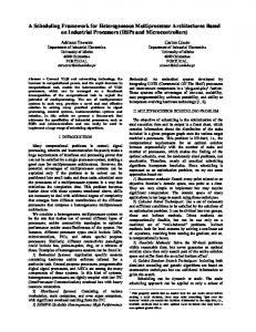
Flow time Θ(log P ) [3, 4] O(1) using (1 + ²)-speed processors [12]

Flow time plus energy O(log P ) using (1 + ²)-speed processors [18] O(1) using (1 + ²)-speed processors [this paper]

Table 1: The competitive ratios of non-migratory online algorithms for minimizing flow time and flow time plus energy. faster. If migration is allowed, SRPT can achieve a competitive ratio one or even smaller, when using sufficiently fast processors [21, 23]. It is worth-mentioning that non-migratory algorithms are preferred in practice because migrating jobs requires overheads and is avoided in many applications. Bunde [9] is the first to study multi-processor scheduling that takes both flow time and energy into consideration, his work is about offline approximation for jobs of unit size. Recently, Lam et al. [18] gave the first online algorithm for minimizing flow time plus energy for jobs of arbitrary size; their algorithm is non-migratory and is O(log P )-competitive when using processors with slightly higher maximum speed. They also showed an Ω(log P ) lower bound if extra speed is not allowed. The literature also contains multi-processor results on optimizing other classical objectives together with energy.1 To save energy in the multi-processor setting, one would like to balance the load of the processors so as to avoid running any processor at high speed, and it is natural to consider some kind of roundrobin strategy. Lam et al. [18] in particular considered the online algorithm CRR (classified round robin), which divides jobs into different classes according to their sizes and dispatches jobs of the same class to the processors in a round-robin fashion. They showed that CRR can lead to an O(log P )-competitive algorithm for flow time plus energy. In the bounded speed model, this algorithm requires the processors to have maximum speed (1 + ²)T for any ² > 0. As mentioned before, when flow time is the only concern, (1 + ²) times faster processors can lead to O(1)competitive algorithm even if the online algorithm is required to be non-migratory [12]. Thus, it is natural to ask whether there exists an O(1)-competitive algorithm for flow time plus energy when extra speed is allowed. Our contribution. In this paper, we give an enhanced analysis of CRR for optimizing flow time plus energy on m ≥ 2 processors, and show that CRR can be O(1)-competitive when using processors with slightly higher maximum speed. Table 1 shows a summary of non-migratory results on scheduling for flow time with or without energy concern. The core of our analysis is to prove that there always exists a non-migratory schedule that dispatches jobs according to CRR and whose flow time plus energy is within a constant factor (instead of a factor of O(log P )) of the optimal migratory offline schedule. As a result, we can dispatch jobs in an online fashion by using CRR. And we can approximate the optimal schedule of each processor by using the online algorithm BPS [5, 7] or SRPT-AJC [19] separately for each processor. Since these algorithms are O(1)-competitive for minimizing flow time plus energy in the single-processor setting, they can support CRR to give a competitive result for the multi-processor setting. The performance of CRR plus SRPT-AJC, denoted as CRR-SA, in the bounded speed 1

Pruhs et al. [26] and Bunde [9] both studied offline algorithms for the makespan objective. Albers et al. [2] studied online algorithms for scheduling jobs with restricted deadlines.

3

model (where T denotes the maximum speed) is summarized as below.2 It is convenient to define a constant η² = (1 + ²)α [(1 + ²)α−1 + (1 − 1/α)(2 + ²)/²2 ] for any ² > 0. Following [19], β is defined α−1 as 2(α + 1)/(α − (1+α) 1/(α−1) ). • Against the optimal (offline) non-migratory schedule: For any ² > 0, CRR-SA can be (2η² β)competitive for minimizing flow time plus energy, when the maximum allowable speed is relaxed to (1 + ²)2 T . E.g., if α = 2 and ² = 0.6, the competitive ratio is about 96; if α = 3 and ² = 0.1, the competitive ratio is 1504. • Against the optimal (offline) migratory schedule: The competitive ratio becomes 5η² β. Both the analyses in [18] and in this paper stem from an offline result to eliminate migration.3 Roughly speaking, the analysis in [18] relies on a transformation of an arbitrary job set to an “mparallel” job set, in which jobs can be divided into groups of m jobs with same release time. For m-parallel job set, it is relatively easy to obtain an optimal non-migratory schedule that dispatches jobs according to CRR using extra speed. Yet transforming an arbitrary job set to an m-parallel job set and vice versa require a non-trivial technique to modify the release times of jobs forward and backward. Such transformation increases the flow time plus energy of the resulting schedule by a factor of O(log P ), and it cannot be improved by using extra speed. In this paper, instead of relying on such transformation, we have an observation that we can focus on some special schedules called “immediate-start” schedules, from which we can derive a much simpler algorithm to construct CRR schedules and exploit the extra speed to show that the flow time plus energy increases by only a constant factor (rather than an O(log P ) factor). Remarks for fixed-speed scheduling. The analysis of CRR also reveals its performance in the context of traditional flow-time scheduling, where processors are of fixed-speed and the concern is on flow time only. In this case, CRR (plus SRPT for individual processor) would give a nonmigratory online algorithm which, when compared with the optimal migratory algorithm, can have a competitive ratio of one or even any constant arbitrarily smaller than one, when using sufficiently fast processors. The competitive ratio can be (56.72/s) when using s-speed processors for s ≥ 56.72.4 Note that if migration is allowed, the efficiency can be much better as McCullough and Torng [21] have showed that the migratory algorithm SRPT is 1s -competitive when using s1 speed processors, where s ≥ 2 − m .

1.1

Preliminaries

Definitions and notations. Given a job set J , we want to schedule J on a pool of m ≥ 2 processors.

Note that jobs are sequential in nature and cannot be executed by more than one processor in parallel. All processors are identical and a job can be executed on any processor. Preemption is allowed and a preempted job can be resumed at the point of preemption. We differentiate two 2

Our analysis can also be applied to the unbounded speed model, but it is of less interest. The cost of eliminating migration has been investigated in the classical setting such as deadline scheduling [11,17] and flow time scheduling [3, 4]. 4 Precisely, we can show that for any ² > 0 such that ²52 (2 + ²) ≥ 1, CRR using processors of speed (1 + ²)2 is 5 (2 + ²)-competitive. Combining with the result of McCullough and Torng [21] that SRPT is 1s -competitive for ²2 single processor when using processor of speed s, this implies CRR using processors of speed s(1 + ²)2 is s²52 (2 + ²)competitive. By changing variables, we can show that with σ = 56.72, CRR using processors of speed s ≥ σ is √ √ 5σ( σ+1) 5σ( σ+1) √ √ -competitive, and ≈ 56.72. 2 2 s( σ−1) ( σ−1) 3

4

types of schedules: a migratory schedule can move partially-executed jobs from one processor to another processor without any penalty, and a non-migratory schedule cannot. We use r(j) and p(j) to denote respectively the release time and work requirement (or size) of P job j. We let p(J ) = j∈J p(j) be the total size of J . The time required to complete job j using a processor with fixed speed s is p(j)/s. With respect to a schedule S for a job set J , we use the notations max-speed(S), EJ (S) and FJ (S) to denote the maximum speed, energy usage, and total flow time, respectively. It is convenient to define GJ (S) = FJ (S)+EJ (S). When the context is clear, we will omit the subscript J . Note that F (S) is the sum, over all jobs, of the time since a job is released until it is completed, or equivalently, the integration over time of the number of unfinished jobs. As processor speed can vary dynamically and the time to execute a job j is not necessarily equal to p(j), we define the execution time of job j to be the flow time minus the waiting time of j, and define the total execution time of S to be the sum of the execution time over all jobs in S. Properties of m-processor schedules. The following lemma shows a lower bound on G(S) which depends on p(J ), irrelevant of the number of processors. Lemma 1. For any m-processor schedule S for a job set J , G(S) ≥

α p(J ). (α−1)1−1/α

Proof. Suppose that a job j in S has flow time t. The energy usage for j is minimized if j is run at constant speed p(j)/t throughout, and it is at least (p(j)/t)α t = p(j)α /tα−1 . Since t + p(j)α /tα−1 is minimized when t = (α − 1)1/α p(j), we have t + p(j)α /tα−1 ≥ (α−1)α1−1/α p(j). Summing over all jobs, we obtain the desired lower bound. We also observe the following property of any optimal schedule. Lemma 2. Any optimal schedule runs a job at the same speed throughout its lifespan. Proof. This is due to the convexity of the power function sα . In any migratory or non-migratory schedule, if a job j is not run at the same speed throughout its lifespan, we can always reduce the energy consumption as follows. Let I be the set of time intervals during which j is run, and let s(t) be the speed that j Ris run at time t (note by at most one processor at t). By ¡R that j is processed ¢α α Jensen’s Inequality, t∈I s(t) dt > |I| · t∈I s(t)dt/|I| , i.e., running j at the average speed over the intervals in I reduces the energy. Critical speed. Without loss of generality, we can assume that at any time an optimal schedule

never runs a job at speed less than the critical speed, defined as 1/(α − 1)1/α [1], and the maximum speed T is at least the critical speed. The assumption stems from an observation (Lemma 4) that a multi-processor schedule can be transformed without increasing the flow time plus energy so that it never runs a job j at speed less than the critical speed. Lemma 4 makes use of a result by Albers and Fujiwara [1] (Lemma 3) that when scheduling a single job j on a single processor for minimizing total flow time plus energy, j should be executed at the critical speed, i.e., 1/(α − 1)1/α . Lemma 3. [1] At any time after a job j has been run on a processor for a while, suppose that we want to further execute j for another x > 0 units of work and minimize the flow time plus energy incurred in this period. The optimal strategy is to let the processor always run at the critical speed.

5

Lemma 4. Given any m-processor schedule S for a job set J , we can construct an m-processor schedule S 0 for J such that S 0 never runs a job at speed less than the critical speed and G(S 0 ) ≤ G(S). Moreover, S 0 needs migration if and only if S does; and max-speed(S 0 ) is at most max{max-speed(S), 1/(α − 1)1/α }. Proof. Assume that there is a time interval I in S during which a processor i is running a job j below the critical speed. If S needs migration, we transform S to a migratory schedule S1 for J such that job j is always scheduled in processor i. This can be done by swapping the schedules of processor i and other processors for different time intervals. If S does not need migration, job j is entirely scheduled in processor i and S1 is simply S. In both cases, G(S1 ) = G(S). We can then improve G(S1 ) by modifying the schedule of processor i as follows. Let x be the amount of work of j processed during I on processor i. First, we schedule this amount of work of j at the critical speed. Note that the time required is shortened. Then we move the remaining schedule of j backward to fill up the time shortened. By Lemma 3, the flow time plus energy for j is preserved. Other jobs in J are left intact. To obtain the schedule S 0 , we repeat this process to eliminate all such intervals I. We can assume that the maximum speed T is at least the critical speed. Otherwise, any multiprocessor schedule including the optimal one would always run a job at the maximum speed. It is because when running a job below the critical speed, the slower the speed, the more total flow time plus energy is incurred. In other words, the problem is reduced to minimizing flow time alone.

2

The online algorithm

This section presents the definition of the online algorithm CRR-SA, which produces a nonmigratory schedule for m ≥ 2 processors. The following three sections are devoted to proving that, when compared with the optimal non-migratory or migratory schedule, this algorithm is O(1)-competitive for flow time plus energy if the maximum allowable speed is slightly relaxed. Consider any fixed constant ² > 0. A job is said to be in class k if its size is in the range ((1 + ²)k−1 , (1 + ²)k ]. In a CRR(²) schedule, jobs of the same class are dispatched upon their arrival to the m processors using a round-robin strategy, and different classes are handled independently. Jobs once dispatched to a processor will be processed there until they finish. Thus a CRR(²) schedule is non-migratory in nature. The intuition of using a CRR schedule comes from a new offline result that there is a CRR schedule such that the total flow time plus energy is O(1) times that of the optimal (non-migratory or migratory) offline schedule and the maximum allowable speed is only slightly higher. Details are stated in Theorem 5 below (Sections 3, 4 and 5 are devoted to proving this theorem). Recall that the constant η² is defined as (1 + ²)α [(1 + ²)α−1 + (1 − 1/α)(2 + ²)/²2 ]. Theorem 5. Given a job set J , let O1 and O2 be respectively an optimal non-migratory schedule and an optimal migratory schedule for J using maximum speed T . Then, for any ² > 0, i. we can construct from O1 a CRR(²) schedule S1 for J such that G(S1 ) ≤ 2η² G(O1 ), and max-speed(S1 ) ≤ (1 + ²)2 × max-speed(O1 ); and ii. we can construct from O2 a CRR(²) schedule S2 for J such that G(S2 ) ≤ 5η² G(O2 ), and max-speed(S2 ) ≤ (1 + ²)2 × max-speed(O2 ). 6

Notice that the CRR schedule stated in Theorem 5 cannot be constructed online. Nevertheless, with Theorem 5, it is natural to design an online algorithm that first dispatches jobs using the policy CRR(²), and then schedules jobs on each processor independently in a way that is competitive in the single-processor setting. For the latter we make use of the single-processor algorithm SRPT-AJC [19]. Below we review the algorithm SRPT-AJC and define the multi-processor algorithm CRR-SA. The definition of SRPT-AJC is for reference only, in this paper we only need to know its performance. Algorithm SRPT-AJC. At any time, run the job with the smallest remaining work at

speed n1/α , where n denotes the number of unfinished jobs at the current time. If n1/α exceeds the maximum allowable speed T , just use the maximum speed T . Algorithm CRR-SA. Jobs are dispatched to the m processors with the CRR(²) policy.

Jobs in each processor are scheduled independently using SRPT-AJC. For a single processor, SRPT-AJC performs well in minimizing flow time plus energy. Lemma 6. [19] For minimizing flow time plus energy of a single processor in the bounded speed α−1 model, SRPT-AJC is β-competitive, where β = 2(α + 1)/(α − (1+α) 1/(α−1) ). Analysis of CRR-SA. With Theorem 5 and Lemma 6, we can easily derive the performance of CRR-SA against the optimal non-migratory or migratory algorithm.

Corollary 7. In the bounded speed model, the performance of CRR-SA for minimizing flow time plus energy on m ≥ 2 processors is as follows. For any ² > 0, i. Against a non-migratory optimal schedule, CRR-SA is 2η² β-competitive when using processors with maximum speed relaxed to (1 + ²)2 T . ii. Against a migratory optimal schedule, CRR-SA is 5η² β-competitive when using processors with maximum speed relaxed to (1 + ²)2 T . Proof. Let O be the optimal non-migratory schedule for a job set J . Consider any ² > 0. By Theorem 5 (i), there exists a CRR(²) schedule S for J such that G(S) ≤ 2η² G(O) and max-speed(S) ≤ (1 + ²)2 × max-speed(O). Let S 0 be the CRR(²) schedule produced by CRR-SA for J . Applying Lemma 6 to individual processors, we conclude that G(S 0 ) ≤ βG(S) ≤ 2η² βG(O), and max-speed(S 0 ) ≤ (1 + ²)2 × max-speed(O). The analysis of the migratory case is the same.

3

Restricted but useful optimal schedules

The remaining three sections are devoted to proving Theorem 5. In essence, for any ² > 0, we want to construct a CRR(²) schedule from an optimal schedule with a mild increase in flow time plus energy and in maximum speed. In this section, we introduce two notions to restrict the possible optimal (non-migratory or migratory) schedules so as to ease the construction. • A job set J is said to be power-of-(1 + ²) if every job in J has size (1 + ²)k for some k. • For any job set J and schedule S, we say that S is immediate-start if every job starts at exactly its release time in J . 7

In general, an optimal schedule may not be immediate-start. The rest of this section shows that it suffices to focus on job sets that are power-of-(1 + ²) and admit optimal schedules that are also immediate-start (such schedules will be referred to as immediate-start, optimal schedules). See Corollary 10 below for a technical summary. The job size restriction is relatively easy to observe as we can exploit a slightly higher maximum speed (Lemma 8). The immediate-start property is non-trivial and perhaps counter-intuitive (Lemma 9). Technically speaking, the results below (Lemmas 8, 9 and Corollary 10) hold in both the migratory and the non-migratory setting. To simplify the presentation of this section, we will not mention whether schedules are migratory or non-migratory. One should read the lemmas and proofs by assuming all schedules are either migratory or non-migratory. Lemma 8. Given a job set J , we can construct a power-of-(1 + ²) job set J 0 such that i. any schedule S1 for J defines a schedule S10 for J 0 such that G(S10 ) ≤ (1 + ²)α G(S1 ) and max-speed(S10 ) ≤ (1 + ²) × max-speed(S1 ); and ii. any schedule S20 for J 0 defines a schedule S2 for J with G(S2 ) ≤ G(S20 ) and max-speed(S2 ) = max-speed(S20 ). Proof. J 0 can be constructed from J by rounding up the size of each job in J to the nearest power of (1 + ²). (i) S1 naturally defines a schedule S10 for J 0 as follows. Whenever S1 runs a job j at speed s, S10 runs the corresponding job in S 0 at speed s0 = s × (1 + ²)dlog1+² p(j)e /p(j). Note that s0 ≤ (1 + ²)s, E(S10 ) ≤ (1 + ²)α E(S1 ), and F (S10 ) = F (S1 ). (ii) is obvious as we can apply any schedule S20 for J 0 to schedule J with extra idle time. We now explain why we can focus on optimal schedules that are immediate-start. Unless otherwise stated, an optimal schedule O below means a schedule that has the smallest flow time plus energy among all schedules with maximum speed not exceeding max-speed(O). To ease the discussion, we add a subscript J to the notations F, E, and G to denote that the job set under concern is J . Given a power-of-(1 + ²) job set J1 and an optimal schedule O1 for J1 , Algorithm MakeISO constructs a power-of-(1 + ²) job set J2 and an immediate-start, optimal schedule O2 for J2 and Lemma 9 states the properties of the constructed schedule. Algorithm MakeISO. We first construct O2 from J1 and O1 . The idea is to repeatedly pick two jobs of the same size and swap their schedules in O1 . More specifically, each time we consider all jobs in J1 of a particular size, and swap their schedules so that their release times and start times in O2 are in the same order (note that the speed at any time stays unchanged and ties are broken by job ids). That is, for all i, the job with the i-th smallest release time will take up the schedule of the job with the i-th smallest start time; note that the i-th smallest start time can never be earlier than the i-th smallest release time. Thus, O2 is also a valid schedule for J1 . Next, we modify J1 to J2 , by replacing the release time of each job j with its start time in O2 . Note that the release time of j can only be delayed (and never gets advanced). Any schedule for J2 (including O2 ) is also a valid schedule for J1 . We now show the following properties of the job set and the schedule constructed by MakeISO. Lemma 9. Given a power-of-(1 + ²) job set J1 and an optimal schedule O1 for J1 , Algorithm MakeISO constructs a power-of-(1 + ²) job set J2 and an immediate-start, optimal schedule O2 for J2 with max-speed(O2 ) ≤ max-speed(O1 ). Furthermore, any CRR(²) schedule S2 for J2 defines a CRR(²) schedule S1 for J1 , and if GJ2 (S2 ) ≤ γGJ2 (O2 ) for some γ ≥ 1, then GJ1 (S1 ) ≤ γGJ1 (O1 ). 8

Proof. By construction, O2 is an immediate-start schedule for J2 . We now analyze the relationship between O1 and O2 and show that CRR preserves performance. O1 and O2 incur the same flow time plus energy for J1 . Since O1 and O2 use the same speed at any time, EJ1 (O1 ) = EJ1 (O2 ). Furthermore, at any time, O1 completes a job if and only if O2 completes a (possibly different) job, and thus O1 and O2 always have the same number of unfinished jobs. This means that FJ1 (O1 ) = FJ1 (O2 ) and GJ1 (O1 ) = GJ1 (O2 ). O2 is optimal for J2 (in terms of flow time plus energy). Suppose on the contrary that there is a schedule O0 for J2 with GJ2 (O0 ) < GJ2 (O2 ). Any schedule for J2 , including O0 and O2 , is also a valid schedule for J1 . Note that EJ1 (O0 ) = EJ2 (O0 ), and FJ1 (O0 ) = FJ2 (O0 ) + d, where d is the total delay of release times of all jobs in J2 (when comparing with J1 ). Therefore, GJ1 (O0 ) = GJ2 (O0 ) + d, and similarly for O2 . Thus, if GJ2 (O0 ) < GJ2 (O2 ), then GJ1 (O0 ) = GJ2 (O0 ) + d < GJ2 (O2 ) + d = GJ1 (O2 ) = GJ1 (O1 ) . This contradicts the optimality of O1 for J1 . CRR preserves performance. Consider any CRR(²) schedule S2 for J2 satisfying GJ2 (S2 ) ≤ γGJ2 (O2 ), for some γ ≥ 1. By definition, jobs of the same class are also of same size and have the same order of release times in J1 and J2 . Therefore, S2 is also an CRR(²) schedule for J1 . For total flow time plus energy, GJ1 (S2 ) = GJ2 (S2 ) + d ≤ γGJ2 (O2 ) + d ≤ γ(GJ2 (O2 ) + d) = γGJ1 (O2 ) = γGJ1 (O1 ) . Thus the lemma follows. In summary, the two lemmas above allow us to focus on power-of-(1 + ²) job sets that admit immediate-start, optimal schedules. Corollary 10. Let J be a job set and let O be an optimal schedule for J . For any ² > 0, there exists a power-of-(1 + ²) job set J 0 and a schedule O0 for J 0 that is immediate-start and optimal among all schedules with maximum speed (1 + ²) × max-speed(O). Furthermore, any CRR(²) schedule S 0 for J 0 defines a CRR(²) schedule S for J , and if GJ 0 (S 0 ) ≤ γGJ 0 (O0 ) for some γ ≥ 1, then GJ (S) ≤ γ(1 + ²)α GJ (O). Proof. By Lemma 8 (i), we construct from J and O a power-of-(1 + ²) job set J1 and a schedule S1 for J1 with GJ1 (S1 ) ≤ (1 + ²)α GJ (O) and max-speed(S1 ) ≤ (1 + ²) × max-speed(O). Let O1 be the optimal schedule for J1 with maximum speed (1 + ²) × max-speed(O). Then GJ1 (O1 ) ≤ GJ1 (S1 ) ≤ (1 + ²)α GJ (O). Next we apply Lemma 9 to J1 and O1 , and we obtain J 0 and an immediate start, optimal schedule O0 with maximum speed at most max-speed(O1 ), which is at most (1 + ²)max-speed(O). Furthermore, by Lemma 9 and Lemma 8 (ii), S 0 defines a CRR(²) schedule S for J such that if GJ 0 (S 0 ) ≤ γGJ 0 (O0 ) for some γ ≥ 1, then GJ (S) ≤ γGJ1 (O1 ) ≤ γ(1 + ²)α GJ (O). In the rest of this paper, we further exploit the fact that any optimal schedule runs a job at the same speed throughout its lifespan (Lemma 2). Also, without loss of generality, at any time an optimal schedule never runs a job at speed less than the critical speed, defined as 1/(α − 1)1/α [1], and the maximum speed T is at least the critical speed (see Section 1.1 for justification). 9

4

Constructing CRR schedules

This section presents an algorithm, called MakeCRR, to construct a CRR schedule from an optimal non-migratory or migratory schedule S ∗ for a job set J . By Corollary 10, we focus on the case where J consists of power-of-(1 + ²) jobs only and S ∗ is immediate-start. Note that in a CRR(²) schedule for J , jobs in each class are of identical size, and the round robin policy is effectively applied independently to every subset of jobs of the same size. It is non-trivial to prove that MakeCRR only increases the flow time and energy of the schedule by a moderate amount. Before we detail the algorithm, it is useful to observe the nature of the CRR schedule S to be constructed. The ordering of job execution in S could be very different from S ∗ . Roughly speaking, S only makes reference to the speed used by S ∗ . Recall that in S ∗ , a job is run at the same speed throughout its lifespan. For any job, S determines its speed as the average of a certain subset of (b + 1)m jobs in S ∗ , where b = 1 or 4 depending on whether S ∗ is non-migratory or migratory. The constant b arises from an upper bound of the number of jobs of the same size that have started but not yet finished at any time. We assume that the processors are numbered from 0 to m − 1. Algorithm MakeCRR. The algorithm has a parameter λ > 0 to control the extra speed (we will eventually set λ = ² to derive the desired result). The construction runs in multiple rounds, from the smallest job size to the largest. Let S0 denote the intermediate schedule, which is initially empty and eventually becomes S. We modify S0 in each round to include more jobs. In the round for size p, suppose that J contains n jobs {j1 , j2 , . . . , jn } of size p, arranged in increasing order of release times. It is convenient to define jn+1 = j1 , jn+2 = j2 , etc. For i = 1 to n, let xi be the average speed in S ∗ of the fastest m jobs among the following (b + 1)m jobs: ji , ji+1 , . . . , ji+(b+1)m−1 . We modify S0 by adding a schedule for ji in processor (i mod m): it can start as early as at its release time, runs at constant speed (1+λ)xi , and occupies the earliest possible times, while avoiding times already committed to earlier jobs for processor (i mod m). Performance of the constructed schedule S. To study the performance of S constructed by Algorithm MakeCRR, we need to be very specific about the properties of the job set J and the optimal schedule S ∗ . By Corollary 10, we assume that J consists of power-of-(1 + ²) jobs only and S ∗ is immediate-start. Furthermore, if S ∗ is non-migratory, it is useful to observe the following property. Property 11. Consider any optimal non-migratory schedule for J on m ≥ 2 processors. At any time, for each job size, there are at most m jobs which have started but not yet finished. We call this property m-proceeding. Property 11 holds because in any optimal non-migratory schedule (no matter whether it is immediate-start or not), jobs of the same size dispatched to a processor must work in a FirstCome-First-Serve manner. Otherwise we can shuffle the execution order to First-Come-First-Serve and reduce the total flow time, and the schedule is not optimal. Note that the m-proceeding property may not hold for an optimal migratory schedule. Nevertheless, we observe a weaker property. In Section 5, we will prove that there exists an optimal migratory schedule for J that is 4m-proceeding and immediate-start. Now we are ready to state the performance of the schedule S constructed by Algorithm MakeCRR. Roughly speaking, if S ∗ is immediate-start and m-proceeding (or 4m-proceeding), then S

10

is a CRR schedule with comparable performance. Details are as follows. It is useful to define µ² = (1 + ²)α−1 + (1 − 1/α)(2 + ²)/²2 for any ² > 0. Note that η² = (1 + ²)α µ² . Lemma 12. Consider any ² > 0. Given a power-of-(1 + ²) job set J with an optimal (migratory or non-migratory) schedule S ∗ that is immediate-start and bm-proceeding for some b ≥ 1, Algorithm MakeCRR (with λ = ²) constructs a CRR(²) schedule S for J such that G(S) ≤ (b + 1)µ² G(S ∗ ), and max-speed(S) ≤ (1 + ²) × max-speed(S ∗ ). 5 The rest of this section is devoted to proving Lemma 12. In Section 4.1, we analyze the energy usage. The analysis of flow time is based on an upper bound on the execution time S spends on jobs of certain classes within a period of time. This upper bound is stated and proved in Section 4.2. With this upper bound, we can analyze the flow time in Section 4.3. Before going into the details of Lemma 12, we show how to exploit Lemma 12 to construct a CRR schedule from any (unrestricted) job set and optimal schedule with the flow time and energy as stated in Theorem 5 (which was first mentioned in Section 2). Theorem 5. Given a job set J , let O1 and O2 be respectively an optimal non-migratory schedule and an optimal migratory schedule for J using maximum speed T . Then, for any ² > 0, i. we can construct from O1 a CRR(²) schedule S1 for J such that G(S1 ) ≤ 2η² G(O1 ), and max-speed(S1 ) ≤ (1 + ²)2 × max-speed(O1 ); and ii. we can construct from O2 a CRR(²) schedule S2 for J such that G(S2 ) ≤ 5η² G(O2 ), and max-speed(S2 ) ≤ (1 + ²)2 × max-speed(O2 ). Proof. We prove the non-migratory case only. The migratory case can be proven in the same way. First of all, we apply Corollary 10 on J and O1 , and we obtain a power-of-(1 + ²) job set J 0 and an immediate-start, optimal non-migratory schedule O0 for J 0 with maximum speed (1 + ²) × max-speed(O1 ). Recall that every optimal non-migratory schedule including O0 is m-proceeding. Next, we apply Algorithm MakeCRR to J 0 and O0 and construct a CRR(²) schedule S 0 for J 0 . By Lemma 12, GJ 0 (S 0 ) ≤ 2µ² GJ 0 (O0 ), and max-speed(S 0 ) ≤ (1 + ²) × max-speed(O0 ). By Corollary 10, S 0 also defines a CRR(²) schedule S1 for J such that GJ (S1 ) ≤ 2(1 + ²)α µ² GJ (O1 ). Note that max-speed(S1 ) ≤ (1 + ²) × max-speed(O0 ) ≤ (1 + ²)2 × max-speed(O1 ).

4.1

Speed and energy

We now start to prove Lemma 12, in which the given job set J consists of power-of-(1+²) jobs, S ∗ is an optimal schedule that is immediate-start and bm-proceeding, and S is the schedule constructed by Algorithm MakeCRR. We first note that in S, the speed of a job is (1 + ²) times the average speed of m jobs in S ∗ , so max-speed(S) ≤ (1 + ²) × max-speed(S ∗ ). Next, we consider the energy. Lemma 13. The energy used by S produced by Algorithm MakeCRR is at most (b + 1)(1 + ²)α−1 G(S ∗ ). 5

In general, if Algorithm MakeCRR uses an arbitrary λ, then we have G(S) ≤ (b + 1)((1 + λ)α−1 + (1 − 1/α)(2 + ²)/λ²)G(S ∗ ), and max-speed(S) ≤ (1 + λ) × max-speed(S ∗ ).

11

Proof. We first note that the energy incurred by running a job of size p at constant speed s is sα p/s = sα−1 p, which is a convex function of the speed. Consider m jobs of size p being run at different constant speeds, and let x be their average speed. Running a job of size p at speed x incurs energy at most 1/m times the total energy for running these m jobs. If we further increase the speed to (1 + ²)x, the power increases by a factor of (1 + ²)α , and the running time decreases by a factor of (1 + ²). Thus, the energy usage increases by a factor of (1 + ²)α−1 . In S, running a job at (1 + ²) times the average speed of m jobs in S ∗ requires no more energy than (1 + ²)α−1 /m times the sum of the energy usage of those m jobs in S ∗ . To bound E(S), we use a simple charging scheme: for a job j in S, we charge to every one of the m jobs j 0 chosen for determining the speed of j in Algorithm MakeCRR; the amount to be charged is 1/m times of the energy usage of j 0 in S ∗ . By Algorithm MakeCRR, each job can be charged by at most (b + 1)m jobs. Thus, (1 + ²)α−1 (b + 1)mE(S ∗ ) m ≤ (b + 1)(1 + ²)α−1 E(S ∗ )

E(S) ≤

≤ (b + 1)(1 + ²)α−1 G(S ∗ ) .

4.2

Upper bound on job execution time of S

To analyze the flow time of a job in S, we attempt to upper bound the execution time of other jobs dispatched to the same processor during its lifespan. Lemmas 14 and 15 below look technical, yet the key observation is quite simple—For any processor z, if we consider all jobs that S dispatches to z during an interval I, excluding the last (b + 1) jobs of each class (size), their total execution time is at most `/(1 + ²), where ` is the length of I. Consider any job h0 ∈ J . Let h1 , h2 , . . . , hn be all the jobs in J such that r(h0 ) ≤ r(h1 ) ≤ · · · ≤ r(hn ) and they have the same size as h0 . Suppose that n ≥ im for some i ≥ b + 1. We focus on two sets of jobs: {h0 , h1 , . . . , him−1 } and {h0 , hm , h2m , . . . , h(i−b−1)m }. The latter contains jobs dispatched to the same processor as h0 . Lemma 14 below gives an upper bound on the execution time of S for {h0 , hm , h2m , . . . , h(i−b−1)m } with respect to S ∗ . Roughly speaking, this lemma stems from the fact that S ∗ is immediate-start and bm-proceeding as well as Algorithm MakeCRR sets the speed of S as (1 + ²) times the average speed of certain jobs in S ∗ . Lemma 14. For any job h0 and i ≥ b + 1, suppose him exists. Let t be the execution time of S ∗ for the jobs h0 , h1 , . . . , him−1 during the interval [r(h0 ), r(him )]. Then in the entire schedule of S, the total execution time of the jobs h0 , hm , . . . , h(i−b−1)m is at most t/m(1 + ²). Proof. Since S ∗ is immediate-start, jobs h0 , . . . , him−1 each starts within the interval [r(h0 ), r(him )]. As S ∗ is bm-proceeding, at time r(him ), at most bm jobs among these im jobs have not yet finished, or equivalently, S ∗ has completed at least (i − b)m jobs. Let ∆ denote a set of any (i − b)m such completed jobs. Based on release times, we partition ∆ accordingly into i − b subsets ∆0 , ∆1 , . . . , ∆i−b−1 , each of size exactly m. ∆0 contains the m jobs with smallest release times in ∆, ∆1 contains jobs with the next m smallest release times in ∆, etc. Since ∆ misses out only bm jobs in {h0 , h1 , . . . , him−1 }, each ∆u , for u ∈ {0, . . . , i − b − 1}, is a subset of the (b + 1)m jobs {hum , hum+1 , . . . , hum+(b+1)m−1 }. Because the speed used by S for hum is (1 + ²) times the average speed of the m fastest jobs in hum , hum+1 , . . . , hum+(b+1)m−1 used by S ∗ , 12

which is faster than (1 + ²) times the average speed of ∆u in S ∗ , it follows that the execution time of hum in S is at most 1/m(1 + ²) times the total execution time of ∆u in S ∗ . Summing over all u ∈ {0, . . . , i − b − 1}, the execution time of S for h0 , hm , . . . , h(i−b−1)m is no more than 1/m(1 + ²) times the total execution time of ∆ in S ∗ . In S ∗ , ∆ is only executed during [r(h0 ), r(him )], and the lemma follows. Below is the main result of this section (to be used for analyzing the flow time of S in Section 4.3). Basically, we have proved in Lemma 14 that for any processor z, we can bound the execution time of all jobs that S dispatches to z during an interval I, excluding the last (b + 1) jobs of each class (size). The remaining jobs can be bounded by the fact that the speed used by S ∗ is at least the critical speed 1/(α − 1)1/α (see Section 1.1). Lemma 15. Consider any k and any time interval I of length `. For jobs of size at most (1 + ²)k that are released during I, the total execution time of any processor in S for these jobs is at most `/(1 + ²) + (b + 1)(1 + ²)k+1 · (α − 1)1/α /²(1 + ²). Proof. Consider a particular k 0 ≤ k. Let yk0 be the total execution time over all processors that 0 S ∗ uses for jobs of size (1 + ²)k during the interval I. Consider a particular processor z in S; 0 suppose that S dispatches i jobs of size (1 + ²)k to processor z during I, and denote these i jobs as J 0 = {h00 , h0m , . . . , h0(i−1)m }, arranged in the order of their release times. We claim that the execution time of processor z in S for these i jobs is at most yk0 /m(1 + ²) plus the execution time of S for the last b + 1 jobs of J 0 . This is obvious if J 0 contains b + 1 or fewer jobs. It remains to consider the case when J 0 has i ≥ b + 2 jobs. By Lemma 14, if t is the execution time of S ∗ for h00 , h01 , . . . , h0(i−1)m−1 during [r(h00 ), r(h0(i−1)m )], then S uses no more than t/m(1 + ²) time to execute h00 , h0m , . . . , h0(i−b−2)m . The claim then follows by noticing that t ≤ yk0 , and we only have b + 1 jobs h0(i−b−1)m · · · h0(i−1)m not being counted. Now we sum over all k 0 ≤ k the upper bound of these flow times, i.e., yk0 /m(1 + ²) plus the P execution time of S for the last b + 1 jobs in J 0 . The sum of the first part is k0 ≤k yk0 /m(1 + ²). P P Note that k0 ≤k yk0 is the execution time of S ∗ during I, so k0 ≤k yk0 ≤ m|I| = m`, and the sum of the first part is P ` k0 ≤k yk0 ≤ . m(1 + ²) 1+² The sum of the second part is over at most b+1 jobs for each k 0 . Recall that the speed used by S ∗ is at least the critical speed 1/(α − 1)1/α (see Section 1.1), and the speed used by S is (1 + ²) times the average of some job speeds in S ∗ . Thus the speed used by S for any job is at least (1+²)/(α−1)1/α , 0 0 and the execution time of each job of size (1 + ²)k is at most (1 + ²)k (α − 1)1/α /(1 + ²). Summing over all k 0 the execution time for these jobs, we have 0 k X (b + 1)(1 + ²)k (α − 1)1/α (b + 1)(1 + ²)k+1 (α − 1)1/α < . 1+² ²(1 + ²) 0

k =0

The lemma follows by summing the two parts.

4.3

Flow time

In this section, we show that the flow time of each job in S is O(1/²2 ) times of its job size (Lemma 16), which implies that the total flow time is O(1/²2 )G(S ∗ ) (Corollary 17). Together 13

with Lemma 13, Lemma 12 can be proved. We first bound the flow time of a job of a particular job size in S, making use of Lemma 15. Lemma 16. In S, the flow time of a job of size (1+²)k is at most (b+1)(2+²)(1+²)k (α−1)1/α /²2 . Proof. Consider a job j of size (1 + ²)k that is scheduled on some processor z in S. Let r = r(j), and f be the flow time of j in S, i.e., j completes at time r + f . To determine f , we focus on the scheduling of processor z in the intermediate schedule S0 immediate after Algorithm MakeCRR has scheduled j. Note that f is due to jobs that have been executed in S during [r, r + f ]. They can be partitioned into two subsets: J1 for jobs released at or before r, and J2 for jobs released during (r, r + f ]. Let f1 and f2 be the contribution on f by J1 and J2 , respectively, i.e., f = f1 + f2 . We first consider J1 . Let t be the last time before r such that processor z is idle right before t in S0 . Thus all jobs executed by processor z at or after t, and hence all jobs in J1 , must be released at or after t. By Lemma 15, the execution time of processor z for jobs in J1 is no more than (r − t)/(1 + ²) + [(b + 1)(1 + ²)k+1 (α − 1)1/α /²(1 + ²)]. Since processor z is busy throughout [t, r), the amount of execution time for jobs in J1 remaining at r is at most r − t (b + 1)(1 + ²)k+1 (α − 1)1/α + − (r − t) 1+² ²(1 + ²) ≤

(b + 1)(1 + ²)k+1 (α − 1)1/α . ²(1 + ²)

This implies f1 ≤ (b + 1)(1 + ²)k+1 (α − 1)1/α /²(1 + ²). Next we consider J2 . Since Algorithm MakeCRR schedules jobs from the smallest to the largest size, jobs in J2 are of size at most (1 + ²)k−1 . We apply Lemma 15 to the interval [r, r + f ] for jobs of size at most (1 + ²)k−1 . The execution time of processor z for jobs in J2 , i.e., f2 , is no more than f (b + 1)(1 + ²)k (α − 1)1/α + . 1+² ²(1 + ²) Then we have f = f1 + f2 ≤

f (b + 1)(2 + ²)(1 + ²)k (α − 1)1/α + , ²(1 + ²) 1+²

immediately implying f ≤ (b + 1)(2 + ²)(1 + ²)k (α − 1)1/α /²2 . Summing over all jobs and recalling that G(S ∗ ) ≥ following corollary.

α (α−1)1−1/α

p(J ) (see Lemma 1), we have the

Corollary 17. The total flow time incurred by S produced by Algorithm MakeCRR is at most ((b + 1)(1 − 1/α)(2 + ²)/²2 )G(S ∗ ). By Lemma 13 and Corollary 17, we have G(S) = E(S)+F (S) ≤ (b+1)[(1+²)α−1 +(1−1/α)(2+ ²)/²2 ]G(S ∗ ) = (b + 1)µ² G(S ∗ ). We have also noted that max-speed(S) ≤ (1 + ²) × max-speed(S ∗ ). Hence, Lemma 12 follows.

14

5

Optimal migratory schedules

Algorithm MakeCRR and Lemma 12 can be applied to an optimal migratory schedule as long as it is immediate-start and bm-proceeding for some integer b ≥ 1. Note that the m-proceeding property or even the 4m-proceeding property does not hold for every optimal migratory schedule. Nevertheless, Lemma 18 below shows that at least one optimal schedule satisfies the 4m-proceeding property (i.e., at any time, there are at most 4m jobs of the same size started but not yet completed). Once we know the existence of such schedule, we can apply the construction in Algorithm MakeISO and Lemma 9 to further modify the job set and the schedule to obtain an optimal migratory schedule that is 4m-proceeding and immediate-start (since the only manipulation done by Algorithm MakeISO is to swap the schedule of pairs of jobs). The rest of the arguments then follow, leading to Theorem 5 (ii). Lemma 18. For any job set J , there exists an optimal migratory schedule S ∗ that is 4m-proceeding. The rest of this section is devoted to proving the above lemma. Recall that m-proceeding property holds for every optimal non-migratory schedule. For optimal migratory schedules, we find that some of them, which we call lazy-start optimal migratory schedules, satisfy the 4m-proceeding property. The definition is as follows: Given a schedule S, we define its “start time sequence” to be the sequence of start time of each job, sorted in the increasing order of time. Among all optimal migratory schedules (which may or may not be immediate-start), a lazy-start optimal schedule is the one with lexicographically maximum start time sequence. Such a schedule has the following property. Lemma 19. In a lazy-start optimal schedule, suppose a job j1 starts at time t, while another job j2 of the same size that has already started before t but has not finished at t is not running at t. Then after t, j1 runs whenever j2 runs. Proof. Suppose the contrary, and let t0 be the first time after t that j2 runs but j1 does not. Let p0 be the amount of work processed for j1 during [t, t0 ] when j2 is not running. We divide the analysis into three cases, each arriving at a contradiction. Case 1: j1 is not yet completed by t0 . We can exchange some x > 0 units of work of j2 starting from t0 with the x units of work of j1 starting from t, without changing processor speed at any time. The start time of j1 is thus delayed without changing the start times of other jobs or increasing the energy or flow time, so the original schedule is not lazy-start. Case 2: j1 is completed by t0 , and the amount of work processed for j2 after t0 is at most p0 .

We can exchange all work of j2 after t0 with some work of j1 starting from t. The completion times of j1 and j2 are exchanged, but the total flow time and energy is preserved. The start time of j1 is delayed without changing the start times of other jobs, so the original schedule is not lazy-start. Case 3: j1 is completed by t0 , and the amount of work processed for j2 after t0 is more than p0 . Since j1 and j2 are of the same size, these conditions imply that there must be some work

processed for j1 when both j1 and j2 are running. Furthermore, j2 must be running slower than j1 during this period, otherwise the total amount of work processed for j2 would be larger than the size of j1 , so the two jobs cannot be of the same size. Since jobs run at constant speed in optimal schedules, the speed of j1 is higher than the speed of j2 . Note that j1 lags behind j2 at t but is ahead of j2 at t0 . So there must be a time t0 ∈ (t0 , t) such that j1 and j2 has been processed for the same amount of work. Exchange the scheduling of j1 15

and j2 after t0 gives a schedule with the completion time of j1 and j2 exchanged, while the energy consumption and flow time remain the same. But now j1 and j2 are not running at constant speed, so the schedule is not optimal. Now we are ready to prove Lemma 18 by showing that a lazy-start optimal migratory schedule is 4m-proceeding. Proof of Lemma 18. Given a job set J , let S be a lazy-start optimal migratory schedule. Suppose, for the sake of contradiction, that at some time in S, there are 4m jobs started but not yet finished. Consider these 4m jobs. At the time when the (m + i)-th job j starts, at least i jobs which started earlier must be idle. For each such idling job j 0 , Lemma 19 dictates that after r(j), whenever j 0 runs, j must also be running. In this case, we say that j 0 implies j. Since there are 4m jobs, there are 1 + 2 + · · · + 3m = 32 m(3m + 1) such relations. Thus some job j0 implies at least 23 m(3m + 1)/4m > m other jobs. After all these other jobs are released, they must all run whenever j0 runs. This contradicts that there are only m processors. The lemma follows.

References [1] S. Albers, and H. Fujiwara. Energy-efficient algorithms for flow time minimization. ACM Transactions on Algorithm, 3(4), 2007. [2] S. Albers, F. Muller, and S. Schmelzer. Speed Scaling on parallel processors. In Proceedings of Symposium on Parallelism in Algorithms and Architectures, pages 289–298, 2007. [3] N. Avrahami, and Y. Azar. Minimizing total flow time and total completion time with immediate dispatching. Algorithmica, 47(3):253–268, 2007. [4] B. Awerbuch, Y. Azar, S. Leonardi, and O. Regev. Minimizing the flow time without migration. SIAM Journal on Computing, 31(5):1370–1382, 2002. [5] N. Bansal, H. L. Chan, T. W. Lam, and L. K. Lee. Scheduling for speed bounded processors. In Proceedings of International Colloquium on Automata, Languages and Programming, pages 409-420, 2008. [6] N. Bansal, T. Kimbrel, and K. Pruhs. Dynamic speed scaling to manage energy and temperature. Journal of the ACM, 54(1), 2007. [7] N. Bansal, K. Pruhs and C. Stein. Speed scaling for weighted flow time. In Proceedings of ACM-SIAM Symposium on Discrete Algorithms, pages 805–813, 2007. [8] D. M. Brooks, P. Bose, S. E. Schuster, H. Jacobson, P. N. Kudva, A. Buyuktosunoglu, J. D. Wellman, V. Zyuban, M. Gupta, and P. W. Cook. Power-aware microarchitecture: Design and modeling challenges for next-generation microprocessors. IEEE Micro, 20(6):26–44, 2000. [9] D. P. Bunde. Power-aware scheduling for makespan and flow. Journal of Scheduling, 12(5):489– 500, 2009.

16

[10] H. L. Chan, W. T. Chan, T. W. Lam, L. K. Lee, K. S. Mak, and P. W. H. Wong. Energy efficient online deadline scheduling. In Proceedings of ACM-SIAM Symposium on Discrete Algorithms, pages 795–804, 2007. [11] H. L. Chan, T. W. Lam and K. K. To. Nonmigratory online deadline scheduling on multiprocessors. SIAM Journal on Computing, 34(3):669–682, 2005. [12] C. Chekuri, A. Goel, S. Khanna, and A. Kumar. Multi-processor scheduling to minimize flow time with ² resource augmentation. In Proceedings of ACM Symposium on Theory of Computing, pages 363–372, 2004. [13] C. Chekuri, S. Khanna, and A. Zhu. Algorithms for minimizing weighted flow time. In Proceedings of ACM Symposium on Theory of Computing, pages 84–93, 2001. [14] D. Grunwald, P. Levis, K. I. Farkas, C. B. Morrey, and M. Neufeld. Policies for dynamic clock scheduling. In Proceedings of Symposium on Operating Systems Design and Implementation, pages 73–86, 2000. [15] S. Irani and K. Pruhs. Algorithmic problems in power management. SIGACT News, 32(2):63– 76, 2005. [16] S. Irani, S. Shukla, and R. K. Gupta. Algorithms for power savings. ACM Transactions on Algorithm, 3(4), 2007. [17] B. Kalyanasundaram and K. Pruhs. Eliminating migration in multi-processor scheduling. Journal of Algorithms, 38:2–24, 2001. [18] T. W. Lam, L. K. Lee, I. K. K. To, and P. W. H. Wong. Non-migratory multi-processor scheduling for response time and energy. IEEE Transactions on Parallel and Distributed Systems, 19(11):1527-1539, 2008. [19] T. W. Lam, L. K. Lee, I. K. K. To, and P. W. H. Wong. Speed scaling functions for flow time scheduling based on active job count. In Proceedings of European Symposium on Algorithms, pages 647–659, 2008. [20] S. Leonardi, and D. Raz. Approximating total flow time on parallel machines. Journal of Computer and System Sciences, 73(6):875–891, 2007. [21] J. McCullough and E. Torng. SRPT optimally utilizes faster machines to minimize flow time. ACM Transactions on Algorithms, 5(1), 2008. [22] T. Mudge. Power: A first-class architectural design constraint. Computer, 34(4):52–58, 2001. [23] C. A. Phillips, C. Stein, E. Torng, and J. Wein. Optimal time-critical scheduling via resource augmentation. Algorithmica, 32(2):163–200, 2002. [24] P. Pillai and K. G. Shin. Real-time dynamic voltage scaling for low-power embedded operating systems. In Proceedings of ACM Symposium on Operating Systems Principles, pages 89–102, 2001.

17

[25] K. Pruhs, J. Sgall, and E. Torng. Online scheduling. In J. Leung, editor, Handbook of Scheduling: Algorithms, Models and Performance Analysis, pages 15-1–15-41. CRC Press, 2004. [26] K. Pruhs, R. van Stee, and P. Uthaisombut. Speed scaling of tasks with precedence constraints. Theory of Computing Systems, 43(1):67–80, 2008. [27] K. Pruhs, P. Uthaisombut, and G. Woeginger. Getting the best response for your erg. ACM Transactions on Algorithms, 4(3), 2008. [28] M. Weiser, B. Welch, A. Demers, and S. Shenker. Scheduling for reduced CPU energy. In Proceedings of Symposium on Operating Systems Design and Implementation, pages 13–23, 1994. [29] F. Yao, A. Demers, and S. Shenker. A scheduling model for reduced CPU energy. In Proceedings of Symposium on Foundations of Computer Science, pages 374–382, 1995.

18