Improving Gate-Level Simulation of Quantum Circuits

Improving Gate-Level Simulation of Quantum Circuits∗

arXiv:quant-ph/0309060v2 29 Nov 2003

George F. Viamontes, Igor L. Markov, and John P. Hayes {gviamont, imarkov, jhayes}@eecs.umich.edu The University of Michigan, Advanced Computer Architecture Laboratory Ann Arbor, MI 48109-2122, USA February 1, 2008

Abstract Simulating quantum computation on a classical computer is a difficult problem. The matrices representing quantum gates, and the vectors modeling qubit states grow exponentially with an increase in the number of qubits. However, by using a novel data structure called the Quantum Information Decision Diagram (QuIDD) that exploits the structure of quantum operators, a useful subset of operator matrices and state vectors can be represented in a form that grows polynomially with the number of qubits. This subset contains, but is not limited to, any equal superposition of n qubits, any computational basis state, n-qubit Pauli matrices, and n-qubit Hadamard matrices. It does not, however, contain the discrete Fourier transform (employed in Shor’s algorithm) and some oracles used in Grover’s algorithm. We first introduce and motivate decision diagrams and QuIDDs. We then analyze the runtime and memory complexity of QuIDD operations. Finally, we empirically validate QuIDD-based simulation by means of a general-purpose quantum computing simulator QuIDDPro implemented in C++. We simulate various instances of Grover’s algorithm with QuIDDPro, and the results demonstrate that QuIDDs asymptotically outperform all other known simulation techniques. Our simulations also show that well-known worst-case instances of classical searching can be circumvented in many specific cases by data compression techniques.

∗ Earlier results of this work were reported at ASPDAC ’03 [18]. New material includes significantly better experimental results and a description of a class of matrices and vectors which can be manipulated in polynomial time and memory using QuIDDPro.

1

1 Introduction Richard Feynman observed in the 1980s that simulating quantum mechanical processes on a standard classical computer seems to require super-polynomial memory and time [12]. For instance, a complex vector of size 2n is needed to represent all the information in n quantum states, and square matrices of size 22n are needed to model (simulate) the time evolution of the states [14]. Consequently, Feynman proposed quantum computing which uses the quantum mechanical states themselves to simulate quantum processes. The key idea is to replace bits with quantum states called qubits as the fundamental units of information. A quantum computer can operate directly on exponentially more data than a classical computer with a similar number of operations and information units. Thus in addressing the problem of simulating quantum mechanical processes more efficiently, Feynman discovered a new computing model that can outperform classical computation in certain cases. Software simulation has long been an invaluable tool for the design and testing of digital circuits. This problem too was once thought to be computationally intractable. Early simulation and synthesis techniques for n-bit circuits often required O(2n ) runtime and memory, with the worst-case complexity being fairly typical. Later algorithmic advancements brought about the ability to perform circuit simulation much more efficiently in practical cases. One such advance was the development of a data structure called the Reduced Ordered Binary Decision Diagram (ROBDD) [5], which can greatly compress the Boolean description of digital circuits and allow direct manipulation of the compressed form. Software simulation may also play a vital role in the development of quantum hardware by enabling the modeling and analysis of large-scale designs that cannot be implemented physically with current technology. Unfortunately, straightforward simulation of quantum designs by classical computers executing standard linear-algebraic routines requires O(2n ) time and memory [12, 14]. However, just as ROBDDs and other innovations have made the simulation of very large classical computers tractable, new algorithmic techniques can allow the efficient simulation of quantum computers. The goal of the work reported here is to develop a practical software means of simulating quantum computers efficiently on classical computers. We propose a new data structure called the Quantum Information Decision Diagram (QuIDD) which is based on decision diagram concepts that are well-known in the context of simulating classical computer hardware [6, 2, 5]. As we demonstrate, QuIDDs allow simulations of n-qubit systems to achieve run-time and memory complexities that range from O(1) to O(2n ), and the worst case is not typical. In the important case of Grover’s quantum search algorithm [11], we show that our QuIDD-based simulator outperforms all other known simulation techniques. The paper is organized as follows. Section 2 outlines previous work on decision diagrams and the modeling of quantum computation on classical computers. In Section 3 we present our QuIDD data structure. Section 4 analyzes the runtime and memory complexity of QuIDD operations, while Section 5 describes some experimental results using QuIDDs. Finally, in Section 6 we present our conclusions and ideas for future work.

2 Background This section first presents the basic concepts of decision diagrams, assuming only a rudimentary knowledge of computational complexity and graph theory. It then reviews previous research on simulating quantum mechanical matrix operations.

2.1 Binary Decision Diagrams The binary decision diagram (BDD) was introduced by Lee in 1959 [13] in the context of classical logic circuit design. This data structure represents a Boolean function f (x1 , x2 , ..., xn ) by a directed acyclic graph (DAG); see Figure 1. By convention, the top node of a BDD is labeled with the name of the function f represented by the BDD. Each variable xi of f is associated with one or more nodes with two outgoing edges labeled then (solid line) and else (dashed line). The then edge of node xi denotes an assignment of logic 1 to the xi , while the else edge represents an assignment of logic 0. These nodes are called internal nodes and are labeled by the corresponding variable xi . The edges of the BDD point downward, implying a top-down assignment of values to the Boolean variables depicted by the internal nodes.

2

f

f x0

x0 x1

f = x0 · x1 + x1 1 (a)

x1

x1 0

1

0

(b)

f

1

x1

0

1

(c)

0 (d)

Figure 1: (a) A logic function, (b) its BDD representation, (c) its BDD representation after applying the first reduction rule, and (d) its ROBDD representation.

At the bottom of the BDD are terminal nodes containing the logic values 1 or 0. They denote the output value of the function f for a given assignment of its variables. Each path through the BDD from top to bottom represents a specific assignment of 0-1 values to the variables x1 , x2 , ..., xn of f , and ends with the corresponding output value f (x1 , x2 , ..., xn ). The original BDD data structure conceived by Lee has exponential worst-case memory complexity Θ(2n ), where n is the number of Boolean variables in a given logic function. Moreover, exponential memory and runtime are required in many practical cases, making this data structure impractical for simulation of large logic circuits. To address this limitation, Bryant developed the Reduced Ordered BDD (ROBDD) [5], where all variables are ordered, and decisions are made in that order. A key advantage of the ROBDD is that variable-ordering facilitates an efficient implementation of reduction rules that automatically eliminate redundancy from the basic BDD representation and may be summarized as follows: 1. There are no nodes v and v′ such that the subgraphs rooted at v and v′ are isomorphic 2. There are no internal nodes with then and else edges that both point to the same node An example of how the rules transform a BDD into an ROBDD is shown in Figure 1. The subgraphs rooted at the x1 nodes in Figure 1b are isomorphic. By applying the first reduction rule, the BDD in Figure 1b is converted into the BDD in Figure 1c. Notice that in this new BDD, the then and else edges of the x0 node now point to the same node. Applying the second reduction rule eliminates the x0 node, producing the ROBDD in Figure 1d. Intuitively it makes sense to eliminate the x0 node since the output of the original function is determined solely by the value of x1 . An important aspect of redundancy elimination is the sensitivity of ROBDD size to the variable ordering. Finding the optimal variable ordering is an NP-complete problem, but efficient ordering heuristics have been developed for specific applications. Moreover, it turns out that many practical logic functions have ROBDD representations that are polynomial (or even linear) in the number of input variables [5]. Consequently, ROBDDs have become indispensable tools in the design and simulation of classical logic circuits.

2.2 BDD Operations Even though the ROBDD is often quite compact, efficient algorithms are necessary to make it practical for circuit simulation. Thus, in addition to the foregoing reduction rules, Bryant introduced a variety of ROBDD operations whose complexities are bounded by the size of the ROBDDs being manipulated [5]. Of central importance is the Apply operation, which performs a binary operation with two ROBDDs, producing a third ROBDD as the result. It can be used, for example, to compute the logical AND of two functions. Apply is implemented by a recursive traversal of the two ROBDD operands. For each pair of nodes visited during the traversal, an internal node is added to the resultant ROBDD using the three rules depicted in Figure 2. To

3

understand the rules, some notation must be introduced. Let v f denote an arbitrary node in an ROBDD f . If v f is an internal node, Var(v f ) is the Boolean variable represented by v f , T (v f ) is the node reached when traversing the then edge of v f , and E(v f ) is the node reached when traversing the else edge of v f . Rule 1

Rule 2

Rule 3

xi

xi

xi

Apply(T(v f ),vg ,op)

Apply(v f ,T(vg ),op)

Apply(T(v f ),T(vg ),op)

Apply(E(vf ),vg ,op)

xi ≺ x j

Apply(v f ,E(vg ),op)

xi ≻ x j

Apply(E(v f ),E(vg ),op)

xi = x j

Figure 2: The three recursive rules used by the Apply operation which determine how a new node should be added to a resultant ROBDD. In the figure, xi = Var(v f ) and x j = Var(vg ). The notation xi ≺ x j is defined to mean that xi precedes x j in the variable ordering. Clearly the rules depend on the variable ordering. To illustrate, consider performing Apply using a binary operation op and two ROBDDs f and g. Apply takes as arguments two nodes, one from f and one from g, and the operation op. This is denoted as Apply(v f , vg , op). Apply compares Var(v f ) and Var(vg ) and adds a new internal node to the ROBDD result using the three rules. The rules also guide Apply’s traversal of the then and else edges (this is the recursive step). For example, suppose Apply(v f , vg , op) is called and Var(v f ) ≺ Var(vg ). Rule 1 is invoked, causing an internal node containing Var(v f ) to be added to the resulting ROBDD. Rule 1 then directs the Apply operation to call itself recursively with Apply(T (v f ), vg , op) and Apply(E(v f ), vg , op). Rules 2 and 3 dictate similar actions but handle the cases when Var(v f ) ≻ Var(vg ) and Var(v f ) = Var(vg ). To recurse over both ROBDD operands correctly, the initial call to Apply must be Apply(Root( f ), Root(g), op) where Root( f ) and Root(g) are the root nodes for the ROBDDs f and g. The recursion stops when both v f and vg are terminal nodes. When this occurs, op is performed with the values of the terminals as operands, and the resulting value is added to the ROBDD result as a terminal node. For example, if v f contains the value logical 1, vg contains the value logical 0, and op is defined to be ⊕ (XOR), then a new terminal with value 1 ⊕ 0 = 1 is added to the ROBDD result. Terminal nodes are considered after all variables are considered. Thus, when a terminal node is compared to an internal node, either Rule 1 or Rule 2 will be invoked depending on which ROBDD the internal node is from. ROBDD variants have been adopted in several contexts outside the domain of logic design. Of particular relevance to this work are Multi-Terminal Binary Decision Diagrams (MTBDDs) [6] and Algebraic Decision Diagrams (ADDs) [2]. These data structures are compressed representations of matrices and vectors rather than logic functions, and the amount of compression achieved is proportional to the frequency of repeated values in a given matrix or vector. Additionally, some standard linear-algebraic operations, such as matrix multiplication, are defined for MTBDDs and ADDs. Since they are based on the Apply operation, the efficiency of these operations is proportional to the size in nodes of the MTBDDs or ADDs being manipulated. Further discussion of the MTBDD and ADD representations is deferred to Subsection 3.1 where the general structure of the QuIDD is described.

2.3 Previous Linear-Algebraic Techniques Quantum-circuit simulators must support linear-algebraic operations such as matrix multiplication, the tensor product, and the projection operators. They typically employ array-based methods to multiply matrices and so require exponential computational resources in the number of qubits. Such methods are often insensitive to the actual values stored, and even sparse-matrix storage offers little improvement for quantum operators with no zero matrix elements, such as Hadamard operators. Several clever matrix methods have been developed for quantum simulation. For example, one can simulate k-input quantum gates on an n-qubit state vector (k ≤ n) without explicitly storing a 2n × 2n matrix representation. The basic idea is to simulate the full-fledged matrix-vector multiplication by a series of simpler operations. To illustrate, consider simulating a quantum circuit in which a 1-qubit Hadamard

4

operator is applied to the third qubit of the state-space |00100i. The state vector representing this statespace has 25 elements. A naive way to apply the 1-qubit Hadamard is to construct a 25 × 25 matrix of the form I ⊗ I ⊗ H ⊗ I ⊗ I and then multiply this matrix by the state vector. However, rather than compute (I ⊗ I ⊗ H ⊗ I ⊗ I)|00100i, one can simply compute |00i ⊗ H|1i ⊗ |00i, which produces the same result using a 2 × 2 matrix H. The same technique can be applied when the state-space is in a superposition, such as α|00100i + β|00000i. In this case, to simulate the application of a 1-qubit Hadamard operator to the third qubit, one can compute |00i ⊗ H(α|1i + β|0i) ⊗ |00i. As in the previous example, a 2 × 2 matrix is sufficient. While the above method allows one to compute a state space symbolically, in a realistic simulation environment, state vectors may be much more complicated. Shortcuts that take advantage of the linearity of matrix-vector multiplication are desirable. For example, a single qubit can be manipulated in a state vector by extracting a certain set of two-dimensional vectors. Each vector in such a set is composed of two probability amplitudes. The corresponding qubit states for these amplitudes differ in value at the position of the qubit being operated on but agree in every other qubit position. The two-dimensional vectors are then multiplied by matrices representing single qubit gates in the circuit being simulated. We refer to this technique as qubit-wise multiplication because the state-space is manipulated one qubit at a time. Obenland implemented a technique of this kind as part of a simulator for quantum circuits [15]. His method applies one- and two-qubit operator matrices to state vectors of size 2n . Unfortunately, in the best case where k = 1, this only reduces the runtime and memory complexity from O(22n ) to O(2n ), which is still exponential in the number of qubits. Gottesman developed a simulation method involving the Heisenberg representation of quantum computation which tracks the commutators of operators applied by a quantum circuit [9]. With this model, the state vector need not be represented explicitly because the operators describe how an arbitrary state vector would be altered by the circuit. Gottesman showed that simulation based on this model requires only polynomial memory and runtime on a classical computer in certain cases. However, it appears limited to the Clifford and Pauli groups of quantum operators, which do not form a universal gate library. Other advanced simulation techniques including MATLAB’s “packed” representation, apply data compression to matrices and vectors, but cannot perform matrix-vector multiplication on compressed matrices and vectors. A notable exception is Greve’s simulation of Shor’s algorithm which uses BDDs [10]. Probability amplitudes of individual qubits are modeled by single decision nodes. This only captures superpositions where every participating qubit is rotated by ±45 degrees from |0i toward |1i. Another BDD-based technique was recently proposed by Al-Rabadi et al. [1] which can perform multi-valued quantum logic. A drawback of this technique is that it is limited to synthesis of quantum logic gates rather than simulation of their behavior. Though Greve’s and Al-Rabadi et al.’s BDD representations cannot simulate arbitrary quantum circuits, the idea of modeling quantum states with a BDD-based structure is appealing and motivates our approach. Unlike previous techniques, this approach is capable of simulating arbitrary quantum circuits while offering performance improvements as demonstrated by the results presented in Sections 4 and 5.

3 QuIDD Theory The Quantum Information Decision Diagram (QuIDD) was born out of the observation that vectors and matrices which arise in quantum computing exhibit repeated structure. Complex operators obtained from the tensor product of simpler matrices continue to exhibit common substructures which certain BDD variants can capture. MTBDDs and ADDs, introduced in Subsection 2.2, are particularly relevant to the task of simulating quantum systems. The QuIDD can be viewed as an ADD or MTBDD with the following properties: 1. The values of terminal nodes are restricted to the set of complex numbers 2. Rather than contain the values explicitly, QuIDD terminal nodes contain integer indices which map into a separate array of complex numbers. This allows the use of a simpler integer function for Apply-based operations, along with existing ADD and MTBDD libraries [17], greatly reducing implementation overhead. 3. The variable ordering of QuIDDs interleaves row and column variables, which favors compression of block patterns (see Subsection 3.2)

5

Vector representation

I0

(a)

0

1/2 00 1/2 01 1/2 10 1/2 11

1/2

I1 0

1

I1 2

3

0.80 −0.10 0.44 0.26

0

0

1

I0

(b)

2

3

0.26 00 0.44 01 −0.10 10 0.80 11

(c)

I1

I1

0

1

1/2 00 −1/2 01 −1/2 10 1/2 11

−1/2 1/2 0

1

QuIDD representation Figure 3: Sample QuIDDs for state vectors of (a) best, (b) worst and (c) midrange size. 4. Bahar et al. note that ADDs can be padded with 0’s to represent arbitrarily sized matrices [2]. No such padding is necessary in the quantum domain where all vectors and matrices have sizes that are a power of 2 (see Subsection 3.2) As we demonstrate using our QuIDD-based simulator QuIDDPro these properties greatly enhance performance of quantum computational simulation.

3.1 Vectors and Matrices Figure 3 shows the QuIDD structure for three 2-qubit states. We consider the indices of the four vector elements to be binary numbers, and define their bits as decision variables of QuIDDs. A similar definition is used for ADDs [2]. For example, traversing the then edge (solid line) of node I0 in Figure 3c is equivalent to assigning the value 1 to the first bit of the 2-bit vector index. Traversing the else edge (dotted line) of node I1 in the same figure is equivalent to assigning the value 0 to the second bit of the index. These traversals bring us to the terminal value − 21 , which is precisely the value at index 10 in the vector representation. QuIDD representations of matrices extend those of vectors by adding a second type of variable node and enjoy the same reduction rules and compression benefits. Consider the 2-qubit Hadamard matrix annotated with binary row and column indices shown in Figure 4a. In this case there are two sets of indices: The first (vertical) set corresponds to the rows, while the second (horizontal) set corresponds to the columns. We assign the variable name Ri and Ci to the row and column index variables respectively. This distinction between the two sets of variables was originally noted in several works including that of Bahar et al. [2]. Figure 4b shows the QuIDD form of this sample matrix where it is used to modify the state vector |00i = (1, 0, 0, 0) via matrix-vector multiplication, an operation discussed in more detail in Subsection 3.4.

3.2 Variable Ordering As explained in Subsection 2.1, variable ordering can drastically affect the level of compression achieved in BDD-based structures such as QuIDDs. The CUDD programming library [17], which is incorporated into QuIDDPro, offers sophisticated dynamic variable-reordering techniques that achieve performance improvements in various BDD applications. However, dynamic variable reordering has significant time overhead, whereas finding a good static ordering in advance may be preferable in some cases. Good variable orderings are highly dependent upon the structure of the problem at hand, and therefore one way to seek out a good ordering is to study the problem domain. In the case of quantum computing, we notice that all matrices

6

R0

R0 R1  00

         

01 10 11

1 2

1 2

1 2

1 2

− 12

1 2

1 2

1 2

− 12

1 2 00

− 12 01

− 12 10

1 2



  1  −2    1  −2   

C0

C0

*

R1

3

R1 C1

C1

C1

3

2

1 2 11

0 0

1

0

1

1

−1/2 1/2 3

2

C0C1 (a)

(b)

Figure 4: (a) 2-qubit Hadamard, and (b) its QuIDD representation multiplied by |00i = (1, 0, 0, 0). Note that the vector and matrix QuIDDs share the entries in a terminal array that is global to the computation. and vectors contain 2n elements where n is the number of qubits represented. Additionally, the matrices are square and non-singular [14]. McGeer et al. demonstrated that ADDs representing certain rectangular matrices can be operated on efficiently with interleaved row and column variables [7]. Interleaving implies the following variable ordering: R0 ≺ C0 ≺ R1 ≺ C1 ≺ ... ≺ Rn ≺ Cn . Intuitively, the interleaved ordering causes compression to favor regularity in block sub-structures of the matrices. We observe that such regularity is created by tensor products that are required to allow multiple quantum gates to operate in parallel and also to extend smaller quantum gates to operate on larger numbers of qubits. The tensor product A ⊗ B multiplies each element of A by the whole matrix B to create a larger matrix which has dimensions MA · MB by NA · NB . By definition, the tensor product will propagate block patterns in its operands. To illustrate the notion of block patterns and how QuIDDs take advantage of them, consider the tensor product of two one-qubit Hadamard operators: 

√ (1/√2) (1/ 2)

√   √ (1/ √2) (1/√2) ⊗ −1/ 2 (1/ 2)

√  (1/ √2) −1/ 2

=

 

1/2  1/2    1/2 1/2

 1/2 −1/2  1/2 −1/2



1/2 1/2 1/2 −1/2 −1/2 −1/2 −1/2 1/2

    

The above matrices have been separated into quadrants, and each quadrant represents a block. For the Hadamard matrices depicted, three of the four blocks are equal in both of the one-qubit matrices and also in the larger two-qubit matrix (the equivalent blocks are surrounded by parentheses). This repetition of equivalent blocks demonstrates that the tensor product of two equal matrices propagates block patterns. In the case of the above example, the pattern is that all but the lower-right quadrant of an n-qubit Hadamard operator are equal. Furthermore, the structure of the two-qubit matrix implies a recursive block sub-structure, which can be seen by recursively partitioning each of the quadrants in the two-qubit matrix:



√ (1/√2) (1/ 2)

√ √   (1/√2) (1/ √2) ⊗ −1/ 2 (1/ 2)

 

(1/2) (1/2)

 √    (1/ √2) =   −1/ 2    (1/2) (1/2)

(1/2) −1/2



(1/2) −1/2





(1/2) (1/2)

(−1/2) (−1/2)

(1/2) −1/2

 

(−1/2) 1/2

      

The only difference between the values in the two-qubit matrix and the values in the one-qubit matrices √ is a factor of 1/ 2. Thus, we can recursively define the Hadamard operator as follows:

7

H

n

H

R0

1

R0

−1/2 1/2 C0

C 2H

0

C0

n−1

C 1H

n−1

0

(a)

1

1 (b)

Figure 5: (a) n-qubit Hadamard QuIDD depicted next to (b) 1-qubit Hadamard QuIDD. Notice that they are isomorphic except at the terminals.

H n−1

⊗ H n−1

=



C1 H n−1 C1 H n−1 C1 H n−1 C2 H n−1



√ √ where C1 = 1/ 2 and C2 = −1/ 2. Other operators constructed via the tensor product can also be defined recursively in a similar fashion. Since three of the four blocks in an n-qubit Hadamard operator are equal, significant redundancy is exhibited. The interleaved variable ordering property allows a QuIDD to explicitly represent only two distinct blocks rather than four as shown in Figure 5. As we demonstrate in Sections 4 and 5, compression of equivalent block sub-structures using QuIDDs offers major performance improvements for many of the operators that are frequently used in quantum computation. In the next Subsection, we describe an algorithm which implements the tensor product for QuIDDs and leads to the compression just described.

3.3 Tensor Product With the structure and variable ordering in place, operations involving QuIDDs can now be defined. Most operations defined for ADDs also work on QuIDDs with some modification to accommodate the QuIDD properties. The tensor (Kronecker) product has been described by Clarke et al. for MTBDDs representing various arithmetic transform matrices [6]. Here we reproduce an algorithm for the tensor product of QuIDDs based on the Apply operation that bears similarity to Clarke’s description. Recall that the tensor product A ⊗ B produces a new matrix which multiplies each element of A by the entire matrix B. Rows (columns) of the tensor product matrix are component-wise products of rows (columns) of the argument matrices. Therefore it is straightforward to implement the tensor product operation on QuIDDs using the Apply function with an argument that directs Apply to multiply when it reaches the terminals of both operands. However, the main difficulty here lies in ensuring that the terminals of A are each multiplied by all the terminals of B. From the definition of the standard recursive Apply routine, we know that variables which precede other variables in the ordering are expanded first [5, 6]. Therefore, we must first shift all variables in B in the current order after all of the variables in A prior to the call to Apply. After this shift is performed, the Apply routine will then produce the desired behavior. Apply starts out with A ∗ B and expands A alone until Aterminal ∗ B is reached for each terminal in A. Once a terminal of A is reached, B is fully expanded, implying that each terminal of A is multiplied by all of B. The size of the resulting QuIDD and the runtime for generating it given two operands of sizes a and b (in number of nodes) is O(ab) because the tensor product simply involves a variable shift of complexity O(b), followed by a call to Apply, which Bryant showed to have time and memory complexity O(ab) [5].

3.4 Matrix Multiplication Matrix multiplication can be implemented very efficiently by using Apply to implement the dot-product operation. This follows from the observation that multiplication is a series of dot-products between the rows

8

of one operand and the columns of the other operand. In particular, given matrices A and B with elements ai j and bi j , their product C = AB can be computed element-wise by ci j = Σnj=1 ai j b ji . Matrix multiplication for QuIDDs is an extension of the Apply function that implements the dot-product. One call to Apply will not suffice because the dot-product requires two binary operations to be performed, namely addition and multiplication. To implement this we simply use the matrix multiplication algorithm defined by Bahar et al. for ADDs [2] but modified to support the QuIDD properties. The algorithm essentially makes two calls to Apply, one for multiplication and the other for addition. Another important issue in efficient matrix multiplication is compression. To avoid the same problem that MATLAB encounters with its “packed” representation, ADDs do not require decompression during matrix multiplication. In the work of Bahar et al., this is addressed by tracking the number i of “skipped” variables between the parent node and its child node in each recursive call. To illustrate, suppose that Var(v f ) = x2 and Var(T (v f )) = x5 . In this situation, i = 5 − 2 = 3. A factor of 2i is multiplied by the terminal-terminal product that is reached at the end of a recursive traversal [2]. The pseudo-code presented for this algorithm in subsequent work of Bahar et al. suggests time-complexity O((ab)2 ) where a and b are the sizes, i.e., the number of decision nodes, of two ADD operands [2]. As with all BDD algorithms based on the Apply function, the size of the resulting ADD is on the order of the time complexity, meaning that the size is also O((ab)2 ). In the context of QuIDDs, we use a modified form of this algorithm to multiply operators by the state vector, meaning that a and b will be the sizes in nodes of a QuIDD matrix and QuIDD state vector, respectively. If either a or b or both are exponential in the number of qubits in the circuit, the QuIDD approach will have exponential time and memory complexity. However, in Section 4 we formally argue that many of the operators which arise in quantum computing have QuIDD representations that are polynomial in the number of qubits. Two important modifications must be made to the ADD matrix multiply algorithm in order to adapt it for QuIDDs. To satisfy QuIDD properties 1 and 2, the algorithm must treat the terminals as indices into an array rather than the actual values to be multiplied and added. Also, a variable ordering problem must be accounted for when multiplying a matrix by a vector. A QuIDD matrix is composed of interleaved row and column variables, whereas a QuIDD vector only depends on column variables. If the ADD algorithm is run as described above without modification, the resulting QuIDD vector will be composed of row instead of column variables. The structure will be correct, but the dependence on row variables prevents the QuIDD vector from being used in future multiplications. Thus, we introduce a simple extension which transposes the row variables in the new QuIDD vector to corresponding column variables. In other words, for each Ri variable that exists in the QuIDD vector’s support, we map that variable to Ci .

3.5 Other Linear-Algebraic Operations Matrix addition is easily implemented by calling Apply with op defined to be addition. Unlike the tensor product, no special variable order shifting is required for matrix addition. Another interesting operation which is nearly identical to matrix addition is element-wise multiplication ci j = ai j bi j . Unlike the dotproduct, this operation involves only products and no summation. This algorithm is implemented just like matrix addition except that op is defined to be multiplication rather than addition. In quantum computer simulation, this operation is useful for matrix-vector multiplications with a diagonal matrix like the Conditional Phase Shift in Grover’s algorithm [11]. Such a shortcut considerably improves upon full-fledged matrix multiplication. Interestingly enough, element-wise multiplication, and matrix addition operations for QuIDDs can perform, without the loss of efficiency, respective scalar operations. That is because a QuIDD with a single terminal node can be viewed both as a scalar value and as a matrix or vector with repeated values. Since matrix addition, element-wise multiplication, and their scalar counterparts are nothing more than calls to Apply, the runtime complexity of each operation is O(ab) where a and b are the sizes in nodes of the QuIDD operands. Likewise, the resulting QuIDD has memory complexity O(ab) [5]. Another relevant operation which can be performed on QuIDDs is the transpose. It is perhaps the simplest QuIDD operation because it is accomplished by swapping the row and column variables of a QuIDD. The transpose is easily extended to the complex conjugate transpose1 by first performing the transpose of a QuIDD and then conjugating its terminal values. The runtime and memory complexity of these operations 1 The

complex conjugate transpose is also known as the Hermitian conjugate or the adjoint.

9

is O(a) where a is the size in nodes of the QuIDD undergoing a transpose. To perform quantum measurement (see Subsection 3.6) one can use the inner product, which can be faster than multiplying by projection matrices and computing norms. Using the transpose, the inner product can be defined for QuIDDs. The inner product of two QuIDD vectors, e.g., hA|Bi, is computed by matrix multiplying the transpose of A with B. Since matrix multiplication is involved, the runtime and memory complexity of the inner product is O((ab)2 ), where a and b are the sizes in nodes of A and B respectively. Our current QuIDD-based simulator QuIDDPro supports matrix multiplication, the tensor product, measurement, matrix addition, element-wise multiplication, scalar operations, the transpose, the complex conjugate transpose, and the inner product.

3.6 Measurement Measurement can be defined for QuIDDs using a combination of operations. After measurement, the state vector is described by: q

Mm |ψi

† hψ|Mm Mm |ψi

Mm is a measurement operator and can be represented by a QuIDD matrix, and the state vector |ψi can be represented by a QuIDD vector. The expression in the numerator involves a QuIDD matrix multiplication. In the denominator, Mm† is the complex conjugate transpose of Mm , which is also defined for QuIDDs. Mm† Mm and Mm† Mm |ψi are matrix multiplications. hψ|Mm† Mm |ψi is an inner product which produces a QuIDD with a single terminal node. Taking the square root of the value in this terminal node is straightforward. To complete the measurement, scalar division is performed with the QuIDD in the numerator and the single terminal QuIDD in the denominator as operands. Let a and b be the sizes in nodes of the measurement operator QuIDD and state vector QuIDD, respectively. Performing the matrix multiplication in the numerator has runtime and memory complexity O((ab)2 ). The scalar division between the numerator and denominator also has the same runtime and memory complexity since the denominator is a QuIDD with a single terminal node. However, computing the denominator will have runtime and memory complexity O(a16 b6 ) due to the matrix-vector multiplications and inner product.

4 Complexity Analyses In this section we prove that the QuIDD data structure can represent a large class of state vectors and operators using an amount of memory that is linear in the number of qubits rather than exponential. Further, we prove that the QuIDD operations required in quantum circuit simulation, i.e., matrix multiplication, the tensor product, and measurement, have both runtime and memory that is linear in the number of qubits for the same class of state vectors and operators. In addition to these complexity issues, we also analyze the runtime and memory complexity of simulating Grover’s algorithm using QuIDDs.

4.1 Complexity of QuIDDs and QuIDD Operations The key to analyzing the runtime and memory complexity of the QuIDD-based simulations lies in describing the mechanics of the tensor product. Indeed, the tensor product is the means by which quantum circuits can be represented with matrices. In the following analysis, the size of a QuIDD is represented by the number of nodes rather than actual memory consumption. Since the amount of memory used by a single QuIDD node is a constant, size in nodes is relevant for asymptotic complexity arguments. Actual memory usage in megabytes of QuIDD simulations is reported in Section 5. Figure 6 illustrates the general form of a tensor product between two QuIDDs A and B. In(A) represents the internal nodes of A, while a1 through ax denote terminal nodes. The notation for B is similar. In(A) is the root subgraph of the tensor product result because of the interleaved variable ordering defined for QuIDDs and the variable shifting operation of the tensor product (see Subsection 3.3). Suppose that A depends on the variables R0 ≺ C0 ≺ . . . ≺ Ri ≺ Ci , and B depends on the variables R0 ≺ C0 ≺ . . . ≺ R j ≺ C j . In performing A ⊗ B, the variables on which B depends will be shifted to Ri+1 ≺ Ci+1 ≺ . . . ≺

10

A

C=A B

In(A)

In(A)

Term(A) a1

...

ax ...

In(B)

B

In(B) Term(C)

In(B)

a 1* b 1

...

a 1* b y

a x*b 1

...

a x*b y

Term(B) b1

...

by

Figure 6: General form of a tensor product between two QuIDDs A and B.

Rk+i+1 ≺ Ck+i+1 . The tensor product is then completed by calling Apply(A, B, ∗). Due to the variable shift on B, Rule 1 of the Apply function will be used after each comparison of a node from A with a node from B until the terminals of A are reached. Using Rule 1 for each of these comparisons implies that only nodes from A will be added to the result, explaining the presence of In(A). Once the terminals of A are reached, Rule 2 of Apply will then be invoked since terminals are defined to appear last in the variable ordering. Using Rule 2 when the terminals of A are reached implies that all the internal nodes from B will be added in place of each terminal of A, causing x copies of In(B) to appear in the result (recall that there are x terminals in A). When the terminals of B are reached, they are multiplied by the appropriate terminals of A. Specifically, the terminals of a copy of B will each be multiplied by the terminal of A that its In(B) replaced. The same reasoning holds for QuIDD vectors as vectors differ in that they depend only on Ri variables. Figure 6 suggests that the size of a QuIDD constructed via the tensor product depends on the number of terminals in the operands. The more terminals a left-hand tensor operand contains, the more copies of the right-hand tensor operand’s internal nodes will be added to the result. More formally, consider the tensor product of a series of QuIDDs ⊗ni=1 Qi = (. . . ((Q1 ⊗ Q2 ) ⊗ Q3 ) ⊗ . . . ⊗ Qn ). Note that the ⊗ operation is associative (thus parenthesis do not affect the result), but it is not commutative. The number of nodes in this tensor product is described by the following lemma. Lemma 4.1 Given QuIDDs {Qi }ni=1 , the tensor-product QuIDD ⊗ni=1 Qi contains n 2 |In(Q1 )| + Σni=2 |In(Qi )||Term(⊗i−1 j=1 Q j )| + |Term(⊗i=1 Qi )| nodes. Proof. This formula can be verified by induction. For the base case, n = 1, there is a single QuIDD Q1 . Putting this information into the formula eliminates the summation term, leaving |In(Q1 )| + |Term(Q1 )| as the total number of nodes in Q1 . This is clearly correct since, by definition, a QuIDD is composed of its internal and terminal nodes. To complete the proof, we now show that if the formula is true for Qn then it’s true for Qn+1 . The inductive hypothesis for Qn is | ⊗ni=1 Qi | = |In(Q1 )| + Σni=2 |In(Qi )||Term(⊗i−1 j=1 Q j )| + 2 |In(A)|

denotes the number of internal nodes in A, while |Term(A)| denotes the number of terminal nodes in A.

11

|Term(⊗ni=1 Qi )|. For Qn+1 the number of nodes is: |(⊗ni=1 Qi ) ⊗ Qn+1| = | ⊗ni=1 Qi | − |Term(⊗ni=1Qi )| + |In(Qn+1)||Term(⊗ni=1 Qi )| + |Term(⊗n+1 i=1 Qi )| Notice that the number of terminals in ⊗ni=1 Qi are subtracted from the total number of nodes in ⊗ni=1 Qi and multiplied by the number of internal nodes in Qn+1 . The presence of these terms is due to Rule 2 of Apply which dictates that in the tensor-product (⊗ni=1 Qi ) ⊗ Qn+1 , the terminals of ⊗ni=1 Qi are replaced by copies of Qn+1 where each copy’s terminals are multiplied by a terminal from ⊗ni=1 Qi . The last term simply accounts for the total number of terminals in the tensor-product. Substituting the inductive hypothesis made earlier for the term | ⊗ni=1 Qi | produces: n n |In(Q1 )| + Σni=2|In(Qi )||Term(⊗i−1 j=1 Q j )| + |Term(⊗i=1 Qi )| − |Term(⊗i=1 Qi )|+ n+1 n |In(Qn+1 )||Term(⊗i=1 Qi )| + |Term(⊗i=1 Qi )| i−1 n+1 = |In(Q1 )| + Σn+1 i=2 |In(Qi )||Term(⊗ j=1 Q j )| + |Term(⊗i=1 )|

Thus the number of nodes in Qn+1 is equal to the original formula we set out to prove for n + 1 and the induction is complete. 2 Lemma 4.1 suggests that if the number of terminals in ⊗i=1 Qi increases by a certain factor with each Qi , then ⊗ni=1 Qi must grow exponentially in n. If, however, the number of terminals stops changing, then ⊗ni=1 Qi must grow linearly in n. Thus, the growth depends on matrix entries because terminals of A ⊗ B are products of terminal values of A by terminal values of B and repeated products are merged. If all QuIDDs Qi have terminal values from the same set Γ, the product’s terminal values are products of elements from Γ. Definition 4.2 Consider finite non-empty sets of complex numbers Γ1 and Γ2 , and define their all-pairs product as {xy | x ∈ Γ1 , y ∈ Γ2 }. One can verify that this operation is associative, and therefore the set Γn of all n-element products is well defined for n > 0. We then call a finite non-empty set Γ ⊂ C persistent iff the size of Γn is constant for all n > 0. For example, the set Γ = {c, −c} is persistent for any c because Γn = {cn , −cn }. In general any set closed under multiplication is persistent, but that is not a necessary condition. In particular, for c 6= 0, the persistence of Γ is equivalent to the persistence of cΓ. Another observation is that Γ is persistent if and only if Γ ∪ {0} is persistent. An important example of a persistent set is the set consisting of 0 and all n-th degree roots of unity Un = {e2πik/n |k = 0..n − 1}, for some n. Since roots of unity form a group, they are closed under multiplication and form a persistent set. In the Appendix, we show that every persistent set is either cUn for some n and c 6= 0, or {0} ∪ cUn. The importance of persistent sets is underlined by the following theorem. Theorem 4.3 Given a persistent set Γ and a constant C, consider n QuIDDs with at most C nodes each and terminal values from a persistent set Γ. The tensor product of those QuIDDs has O(n) nodes and can be computed in O(n) time. Proof. The first and the last terms of the formula in Lemma 4.1 are bounded by C and |Γ| respectively. As the sizes of terminal sets in the middle term are bounded by |Γ|, the middle term is bounded by |Γ| ∑ni=2 |In(Qi )| < |Γ|c since each |In(Qi )| is a constant. The tensor product operation A ⊗ B for QuIDDs involves a shift of variables on B followed by Apply(A, B, ∗). If B is a QuIDD representing n qubits, then B depends on O(n) variables.3 This implies that the runtime of the variable shift is O(n). Bryant proved that the asymptotic runtime and memory complexity of Apply(A, B, binary op) is O(|A||B|) [5]. Lemma 4.1 and the fact that we are considering QuIDDs with at most C nodes and terminals from a persistent set Γ imply that |A| = O(n) and |B| = O(1). Thus, Apply(A, B, ∗) has asymptotic runtime and memory complexity O(n), leading to an overall asymptotic runtime and memory complexity of O(n) for computing ⊗ni=1 Qi . 2 Importantly, the terminal values do not need to form a persistent set themselves for the theorem to hold. If they are contained in a persistent set, then the sets of all possible m-element products (i.e. m ≤ n for

3 More

accurately, B depends on exactly 2n variables if it is a matrix QuIDD and n variables if it is a vector QuIDD.

12

|0>

H

H

X

X

H

|0>

H

H

X

X

H

X

H

X

H

ORACLE |0>

H

H

X

|0>

H

H

X

|0>

|1>

Oracle "work" qubit−space

H

H

CONDITIONAL PHASE SHIFT

|0>

H

H

R Iterations (Boyer’s Formula)

Figure 7: Circuit-level implementation of Grover’s algorithm

all n-element products in a set Γ) eventually stabilize in the sense that their sizes do not exceed that of Γ. However, this is only true for a fixed m rather than for the sets of products of m elements and fewer. For QuIDDs A and B, the matrix-matrix and matrix-vector product computations are not as sensitive to terminal values, but depend on sizes of the QuIDDs. Indeed, the memory and time complexity of this operation is O(|A|2 |B|2 ) [2]. Theorem 4.4 Consider measuring an n-qubit QuIDD state vector |ψi using a QuIDD measurement operator M, where both |ψi and M are constructed via the tensor product of an arbitrary sequence of O(1)-sized QuIDD vectors and matrices, respectively. If the terminal node values of the O(1) − sized QuIDD vectors or operators are in a persistent set Γ, then the runtime and memory complexity of measuring the QuIDD state vector is O(n22 ). Proof. In Subsection 3.6, we showed that runtime and memory complexity for measuring a state vector QuIDD is O(a16 b6 ), where a and b be the sizes in nodes of the measurement operator QuIDD and state vector QuIDD, respectively. From Theorem 4.3, the asymptotic memory complexity of both a and b is O(n), leading to an overall runtime and memory complexity of O(n22 ). 2 The class of QuIDDs described by Theorem 4.3 and its corollaries, with terminals taken from the set {0} ∪ cU, encompasses a large number of practical quantum state vectors and operators. These include, but are not limited to, any equal superposition of n qubits, any sequence of n qubits in the computational basis states, n-qubit Pauli matrices, and n-qubit Hadamard matrices. The above results suggest a polynomialsized QuIDD representation of any quantum circuit on n qubits in terms of such gates if the number of gates is limited by a constant. In other words, the above sufficient conditions apply if the depth (length) of the circuit is limited by a constant. Our simulation technique may use polynomial memory and runtime in other circumstances as well, as shown in the next Subsection.

4.2 Complexity of Grover’s Algorithm using QuIDDs To investigate the power of the QuIDD representation, we used QuIDDPro to simulate Grover’s algorithm [11], one of the two major quantum algorithms that have been developed to date. Grover’s algorithm searches for a subset of items in an unordered database of N items. The only selection criterion available is a black-box predicate that can be evaluated on any item in the database. The complexity of this evaluation

13

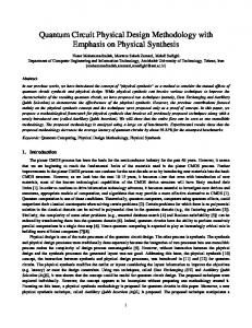
(query) is unknown, and the overall complexity analysis is performed in terms of queries. In the classical domain, any algorithm for such an unordered search must query the predicate √ Ω(N) times. However, Grover’s algorithm can perform the search with quantum query complexity O( N), a quadratic improvement. This assumes that a quantum version of the search predicate can be evaluated on a superposition of all database items. A quantum circuit representation of the algorithm involves five major components: an oracle circuit, a conditional phase shift operator, sets of Hadamard gates, the data qubits, and an oracle qubit. The oracle circuit is a Boolean predicate that acts as a filter, flipping the oracle qubit when it receives as input an n bit sequence representing the items being searched for. In quantum circuit form, the oracle circuit is represented as a series of controlled NOT gates with subsets of the data qubits acting as the control qubits and the oracle qubit receiving the action of the NOT gates. Following the oracle circuit, Hadamard gates put the n data qubits into an equal superposition of all 2n items in the database where 2n = N. Then a sequence of gates H ⊗n−1CH ⊗n−1, where C denotes the conditional phase shift operator, are applied iteratively to the data qubits. Each iteration is termed a Grover iteration [14]. Grover’s algorithm must be stopped after a particular number of iterations when the probability amplitudes of the states representing the items sought are sufficiently boosted. There must be enough iterations to ensure a successful measurement, but after a certain point the probability of successful measurement starts fading, and later changes periodically. In our experiments, we used the tight bound on the number of iterationspformulated by Boyer et al. [4] when the number of solutions M is known in advance: ⌊π/4θ⌋ where θ = M/N. The power of Grover’s algorithm lies in the fact that the data qubits store all N = 2n items in the database as a superposition, allowing the oracle circuit to “find” all items being searched for simultaneously. A circuit implementing Grover’s algorithm is shown in Fig. 7. The algorithm can be summarized as follows: Let N denote the number of elements in the database. 1. Initialize n = ⌈log2 N⌉ qubits to |0i and the oracle qubit to |1i. 2. Apply the Hadamard transform (H gate) to all qubits to put them into a uniform superposition of basis states. 3. Apply the oracle circuit. The oracle circuit can be implemented as a series of one or more CNOT gates representing the search criteria. The inputs to the oracle circuit feed into the control portions of the CNOT gates, while the oracle qubit is the target qubit for all of the CNOT gates. In this way, if the input to this circuit satisfies the search criteria, the state of the oracle qubit is flipped. For a superposition of inputs, those input basis states that satisfy the search criteria flip the oracle qubit in the composite state-space. The oracle circuit uses ancillary qubits as its workspace, reversibly returning them to their original states (shown as |0i in Fig 7). These ancillary qubits will not be operated on by any other step in the algorithm. 4. Apply the H gate to all qubits except the oracle qubit. 5. Apply the Conditional Phase-Shift gate on all qubits except the oracle qubit. This gate negates the probability amplitude of the |000 . . .0i basis state, leaving that of the others unaffected. It can be realized using a combination of X, H and Cn−1 -NOT gates as shown. A decomposition of the Cn−1 -NOT into elementary gates is given in [3]. 6. Apply the H gate to all gates except the oracle qubit. q

N ⌋ and M is the number of keys 7. Repeat steps 3-6 (a single Grover iteration) R times, where R = ⌊ π4 M matching the search criteria [4]. 8. Apply the H gate to the oracle qubit in the last iteration. Measure the first n qubits to obtain the index of the matching key with high probability.

Using explicit vectors and matrices to simulate the above procedure would incur memory and runtime complexities of Ω(2n ). However, this is not necessarily the case when using QuIDDs. To show this, we present a step-by-step complexity analysis for a QuIDD-based simulation of the procedure. Steps 1 and 2 Theorem 4.3 implies that the memory and runtime complexity of step 1 is O(n) because the initial state vector only contains elements in cUk ∪ {0} and is constructed via the tensor product. Step 2 is simply a matrix multiplication of an n-qubit Hadamard matrix with the state vector constructed in step 1. The Hadamard matrix has memory complexity O(n) by Theorem 4.3. Since the state vector also has memory complexity O(n), further matrix-vector multiplication in step 2 has O(n4 ) memory and runtime

14

complexity because computing the product of two QuIDDs A and B takes O((|A||B|)2 ) time and memory [2]. This upper-bound can be trivially tightened, however. The function of these steps is to put the qubits into an equal superposition. For the n data qubits, this produces a QuIDD with O(1) nodes because an 1 . Also, n-qubit state vector representing an equal superposition has only one distinct element, namely 2n/2 applying a Hadamard matrix to the single oracle qubit results in a QuIDD with O(1) nodes because in the worst-case, the size of a 1-qubit QuIDD is clearly a contant. Since the tensor product is based on the Apply algorithm (see Subsection 3.3), the result of tensoring the QuIDD representing the data qubits in an equal superposition with the QuIDD for the oracle qubit is a QuIDD containing O(1) nodes. Steps 3-6 In step 3, the state vector is matrix-multiplied by the oracle matrix. Again, the complexity of multiplying two arbitrary QuIDDs A and B is O((|A||B|)2 ) [2]. The size of the state vector in step 3 is O(1). If the size of the oracle is represented by |A|, then the memory and runtime complexity of step 3 is O(|A|2 ). Similarly, steps 4, 5, and 6 will have polynomial memory and runtime complexity in terms of |A| and n.4 Thus we arrive at the O(|A|16 n14 ) worst-case upper-bound for the memory and runtime complexity of the simulation at step 6. Judging from our empirical data, this bound is typically very loose and pessimistic. Lemma 4.5 The memory and runtime complexity of a single Grover iteration in a QuIDD-based simulation is O(|A|16 n14 ). Proof. Steps 3 − 6 make up a single Grover iteration. Since the memory and runtime complexity of a QuIDD-based simulation after completing Step 6 is O(|A|16 n14 ), the memory and runtime complexity of a single Grover iteration is O(|A|16 n14 ). 2 q N ⌋ Step 7 Step 7 does not involve a quantum operator, but rather it repeats a Grover iteration R = ⌊ π4 M times. As a result, Step 7 induces an exponential runtime for the simulation, since the number of Grover iterations is a function of N = 2n . This is acceptable though because an actual quantum computer would also require exponentially many Grover iterations in order to measure one of the matching keys with a high probability [4]. Ultimately this is the reason why Grover’s algorithm only offers a quadratic and not an exponential speedup over classical search. Since Lemma 4.5 shows that the memory and runtime complexity of a single Grover iteration is polynomial in the size of the oracle QuIDD, one might guess that the memory complexity of Step 7 is exponential like the runtime. However, it turns out that the size of the state vector does not change from iteration to iteration, as shown below. Lemma 4.6 The internal nodes of the state vector QuIDD at the end of any Grover iteration i are equal to the internal nodes of the state vector QuIDD at the end of Grover iteration i + 1. Proof. Each Grover iteration increases the probability of the states representing matching keys while simultaneously decreasing the probability of the states representing non-matching keys. Therefore, at the end of the first iteration, the state vector QuIDD will have a single terminal node for all the states representing matching keys and one other terminal node, with a lower value, for the states representing non-matching keys (there may be two such terminal nodes for non-matching keys, depending on machine precision). The internal nodes of the state vector QuIDD cannot be different at the end of subsequent Grover iterations because a Grover iteration does not change the pattern of probability amplitudes, but only their values. In other words, the same matching states always point to a terminal node whose value becomes closer to 1 after each iteration, while the same non-matching states always point to a terminal node (or nodes) whose value (or values) becomes closer to 0. 2 Lemma 4.7 The total number of nodes in the state vector QuIDD at the end of any Grover iteration i is equal to the total number of nodes in the state vector QuIDD at the end of Grover iteration i + 1. Proof. In proving Lemma 4.6, we showed that the only change in the state vector QuIDD from iteration to iteration is the values in the terminal nodes (not the number of terminal nodes). Therefore, the number of nodes in the state vector QuIDD is always the same at the end of every Grover iteration. 2 Corollary 4.8 In a QuIDD-based simulation, the runtime and memory complexity of any Grover iteration i is equal to the runtime and memory complexity of Grover iteration i + 1. 4 As noted in step 5, the Conditional Phase-Shift operator can be decomposed into the tensor product of single qubit matrices, giving it memory complexity O(n).

15

Proof. Each Grover iteration is a series of matrix multiplications between the state vector QuIDD and several operator QuIDDs (Steps 3−6). The work of Bahar et al. shows that matrix multiplication with ADDs has runtime and memory complexity that is determined solely by the number of nodes in the operands (see Section 3.4) [2]. Since the total number of nodes in the state vector QuIDD is always the same at the end of every Grover iteration, the runtime and memory complexity of every Grover iteration is the same. 2 Lemmas 4.6 and 4.7 imply that Step 7 does not necessarily induce memory complexity that is exponential in the number of qubits. This important fact is captured in the following theorem. Theorem 4.9 The memory complexity of simulating Grover’s algorithm using QuIDDs is polynomial in the size of the oracle QuIDD and the number of qubits.5 Proof. The runtime and memory complexity of a single Grover iteration is O(|A|16 n14 ) (Lemma 4.5), which includes the initialization costs of Steps 1 and 2. Also, the structure of the state vector QuIDD does not change from one Grover iteration to the next (Lemmas 4.6 and 4.7). Thus, the overall memory complexity of simulating Grover’s algorithm with QuIDDs is O(|A|16 n14 ), where |A| is the number of nodes in the oracle QuIDD and n is the number of qubits. 2 While any polynomial-time quantum computation can be simulated in polynomial space, the commonlyused linear-algebraic simulation requires Ω(2n ) space. Also note that the case of an oracle searching for a unique solution (originally considered by Grover) implies that |A| = n. Here, most of the searching will be done while constructing the QuIDD of the oracle, which is an entirely classical operation. As we demonstrate experimentally in Section 5, for some oracles, simulating Grover’s algorithm with QuIDDs has memory complexity Θ(n). Furthermore, simulation using QuIDDs has worst-case runtime complexity O(R|A|16 n14 ), where R is the number of Grover iterations as defined earlier. If |A| grows polynomially with n, this runtime complexity is the same as that of an ideal quantum computer, up to a polynomial factor.

5 Empirical Validation This section discusses problems that arise when implementing a QuIDD-based simulator. It also presents experimental results obtained from actual simulation.

5.1 Implementation Issues Full support of QuIDDs requires the use of complex arithmetic, which can lead to serious problems if numerical precision is not adequately addressed. Complex Number Arithmetic. At an abstract level, ADDs can support terminals of any numerical type, but CUDD’s implementation of ADDs does not. For efficiency reasons, CUDD stores node information in C unions which are interpreted numerically for terminals and as child pointers for internal nodes. However, it is well-known that unions are incompatible with the use of C++ classes because their multiple interpretations hinder the binding of correct destructors. In particular, complex numbers in C++ are implemented as a templated class and are incompatible with CUDD. This was one of the motivations for storing terminal values in an external array (QuIDD property 2). Numerical Precision. Another important issue is the precision of complex numeric types. Over the course of repeated multiplications, the values of some terminals may become very small and induce roundoff errors if the standard IEEE double precision floating-point types are used. This effect worsens for larger circuits. Unfortunately, such round-off errors can significantly affect the structure of a QuIDD by merging terminals that are only slightly different or not merging terminals whose values should be equal, but differ by a small computational error. The use of approximate comparisons with an epsilon works in certain cases but does not scale well, particularly for creating an equal superposition of states (a standard operation in 1 quantum circuits). In an equal superposition, a circuit with n qubits will contain the terminal value 2n/2 in the state vector. With the IEEE double precision floating-point type, this value will be rounded to 0 at 5 We

do not account for the resources required to construct the QuIDD of the oracle.

16

Circuit Size n 20 30 40 50 60 70 80 90 100

Hadamards Initial Repeated 80 83 120 123 160 163 200 203 240 243 280 283 320 323 360 363 400 403

Conditional Phase Shift 21 31 41 51 61 71 81 91 101

Oracles 1 2 99 108 149 168 199 228 249 288 299 348 349 408 399 468 449 528 499 588

Table 1: Size of QuIDDs (# of nodes) for Grover’s algorithm. n = 2048, preventing the use of epsilons for approximate comparison past n = 2048. Furthermore, a static value for epsilon will not work well for different sized circuits. For example, ε = 10−6 may work well for n = 35, but not for n = 40 because at n = 40, all values may be smaller than 10−6 . Therefore, to address the problem of precision, QuIDDPro uses an arbitrary precision floating-point type from the GMP library [8] with the C++ complex template. Precision is then limited to the available amount of memory in the system.

5.2 Results for Simulating Grover’s Algorithm Before starting simulation of an instance of Grover’s algorithm, we construct the QuIDD representations of Hadamard operators by incrementally tensoring together one-qubit versions of their matrices n − 1 times to get n-qubit versions. All other QuIDD operators are constructed similarly. Table 1 shows sizes (in nodes) of respective QuIDDs at n-qubits, where n = 20..100. We observe that memory usage grows linearly in n, and as a result QuIDD-based simulations of Grover’s algorithm are not memory-limited even at 100 qubits. Note that this is consistent with Theorem 4.3. With the operators constructed, simulation can proceed. Tables 2a and 2b show performance measurements for simulating Grover’s algorithm with an oracle circuit that searches for one item out of 2n . QuIDDPro achieves asymptotic memory savings compared to qubit-wise implementations (see Subsection 2.3) of Grover’s algorithm using Blitz++, a high-performance numerical linear algebra library for C++ [19], MATLAB, and Octave, a mathematical package similar to MATLAB. The overall runtimes are still exponential in n because Grover’s algorithm entails an exponential number of iterations, even on an actual quantum computer [4]. We also studied a “mod-1024” oracle circuit that searches for elements whose ten least significant bits are 1 (see Tables 3a and 3b). Results were produced on a 1.2GHz AMD Athlon with 1GB RAM running Linux. Memory usage for MATLAB and Octave is lower-bounded by the size of the state vector and conditional phase shift operator; Blitz++ and QuIDDPro memory usage is measured as the size of the entire program. Simulations using MATLAB and Octave past 15 qubits timed out at 24 hours.

5.3 Impact of Grover Iterations To verify that the QuIDDPro simulation resulted in the exact number of Grover iterations required to generate the highest probability of measuring the items being sought as per the Boyer et al. formulation [4], we tracked the probabilities of these items as a function of the number of iterations. For this experiment, we used four different oracle circuits, each with 11,12, and 13 qubit circuits. The first oracle is called “Oracle N” and represents an oracle in which all the data qubits act as controls to flip the oracle qubit (this oracle is equivalent to Oracle 1 in the last subsection). The other oracle circuits are “Oracle N-1”, “Oracle N-2”, and “Oracle N-3”, which all have the same structure as Oracle N minus 1,2, and 3 controls, respectively. As described earlier, each removal of a control doubles the number of items being searched for in the database. For example, Oracle N-2 searches for 4 items in the data set because it recognizes the bit pattern 111...1dd. Table 4 shows the optimal number of iterations produced with the Boyer et al. formulation for all the instances tested. Figure 8 plots the probability of successfully finding any of the items sought against the number of Grover iterations. In the case of Oracle N, we plot the probability of measuring the single item being searched for. Similarly, for Oracles N-1, N-2, and N-3, we plot the probability of measuring any one

17

n 10 11 12 13 14 15 16 17 18 19 20 21 22 23 24 25 26 27 28 29 30 31 32 33 34 35 36 37 38 39 40

Oracle 1: Runtime (s) Oct MAT B++ 80.6 6.64 0.15 2.65e2 22.5 0.48 8.36e2 74.2 1.49 2.75e3 2.55e2 4.70 1.03e4 1.06e3 14.6 4.82e4 6.76e3 44.7 > 24hrs > 24hrs 1.35e2 > 24hrs > 24hrs 4.09e2 > 24hrs > 24hrs 1.23e3 > 24hrs > 24hrs 3.67e3 > 24hrs > 24hrs 1.09e4 > 24hrs > 24hrs 3.26e4 > 24hrs > 24hrs > 24hrs > 24hrs > 24hrs > 24hrs > 24hrs > 24hrs > 24hrs > 24hrs > 24hrs > 24hrs > 24hrs > 24hrs > 24hrs > 24hrs > 24hrs > 24hrs > 24hrs > 24hrs > 24hrs > 24hrs > 24hrs > 24hrs > 24hrs > 24hrs > 24hrs > 24hrs > 24hrs > 24hrs > 24hrs > 24hrs > 24hrs > 24hrs > 24hrs > 24hrs > 24hrs > 24hrs > 24hrs > 24hrs > 24hrs > 24hrs > 24hrs > 24hrs > 24hrs > 24hrs > 24hrs > 24hrs > 24hrs > 24hrs > 24hrs > 24hrs > 24hrs > 24hrs > 24hrs > 24hrs > 24hrs (a)

QP 0.33 0.54 0.83 1.30 2.01 3.09 4.79 7.36 11.3 17.1 26.2 39.7 60.5 92.7 1.40e2 2.08e2 3.12e2 4.72e2 7.07e2 1.08e3 1.57e3 2.35e3 3.53e3 5.23e3 7.90e3 1.15e4 1.71e4 2.57e4 3.82e4 5.64e4 8.23e4

n 10 11 12 13 14 15 16 17 18 19 20 21 22 23 24 25 26 27 28 29 30 31 32 33 34 35 36 37 38 39 40

Oracle 1: Oct 2.64e-2 5.47e-2 0.105 0.213 0.426 0.837 1.74 3.34 4.59 13.4 27.8 55.6 NA NA NA NA NA NA NA NA NA NA NA NA NA NA NA NA NA NA NA

Peak Memory Usage (MB) MAT B++ QP 1.05e-2 3.52e-2 9.38e-2 2.07e-2 8.20e-2 0.121 4.12e-2 0.176 0.137 8.22e-2 0.309 0.137 0.164 0.559 0.137 0.328 1.06 0.137 0.656 2.06 0.145 1.31 4.06 0.172 2.62 8.06 0.172 5.24 16.1 0.172 10.5 32.1 0.172 NA 64.1 0.195 NA 1.28e2 0.207 NA 2.56e2 0.207 NA 5.12e2 0.223 NA 1.02e3 0.230 NA > 1.5GB 0.238 NA > 1.5GB 0.254 NA > 1.5GB 0.262 NA > 1.5GB 0.277 NA > 1.5GB 0.297 NA > 1.5GB 0.301 NA > 1.5GB 0.305 NA > 1.5GB 0.320 NA > 1.5GB 0.324 NA > 1.5GB 0.348 NA > 1.5GB 0.352 NA > 1.5GB 0.371 NA > 1.5GB 0.375 NA > 1.5GB 0.395 NA > 1.5GB 0.398 (b)

Table 2: Simulating Grover’s algorithm with n qubits using Octave (Oct), MATLAB (MAT), Blitz++ (B++) and our simulator QuIDDPro (QP). > 24hrs indicates that the runtime exceeded our cutoff of 24 hours. > 1.5GB indicates that the memory usage exceeded our cutoff of 1.5GB. Simulation runs that exceed the memory cutoff can also exceed the time cutoff, though we give memory cutoff precedence. NA indicates that after a cutoff of one week, the memory usage was still steadily growing, preventing a peak memory usage measurement.

of the 2, 4, and 8 items being searched for, respectively. By comparing the results in Table 4 with those in Figure 8, it can be easily verified that QuIDDPro uses the correct number of iterations at which measurement is most likely to produce items sought. Also notice that the probabilities, as a function of the number of iterations, follow a sinusoidal curve. It is therefore important to terminate at the exact optimal number of iterations not only from an efficiency standpoint but also to prevent the probability amplitudes of the items being sought from lowering back down toward 0.

18

n 13 14 15 16 17 18 19 20 21 22 23 24 25 26 27 28 29 30 31 32 33 34 35 36 37 38 39 40

Oracle 2: Runtime (s) Oct MAT B++ 1.39e3 1.31e2 2.47 3.75e3 7.26e2 5.42 1.11e4 4.27e3 11.7 3.70e4 2.23e4 24.9 > 24hrs > 24hrs 53.4 > 24hrs > 24hrs 1.13e2 > 24hrs > 24hrs 2.39e2 > 24hrs > 24hrs 5.15e2 > 24hrs > 24hrs 1.14e3 > 24hrs > 24hrs 2.25e3 > 24hrs > 24hrs 5.21e3 > 24hrs > 24hrs 1.02e4 > 24hrs > 24hrs 2.19e4 > 24hrs > 24hrs > 1.5GB > 24hrs > 24hrs > 1.5GB > 24hrs > 24hrs > 1.5GB > 24hrs > 24hrs > 1.5GB > 24hrs > 24hrs > 1.5GB > 24hrs > 24hrs > 1.5GB > 24hrs > 24hrs > 1.5GB > 24hrs > 24hrs > 1.5GB > 24hrs > 24hrs > 1.5GB > 24hrs > 24hrs > 1.5GB > 24hrs > 24hrs > 1.5GB > 24hrs > 24hrs > 1.5GB > 24hrs > 24hrs > 1.5GB > 24hrs > 24hrs > 1.5GB > 24hrs > 24hrs > 1.5GB (a)

Oracle 2: Peak Memory Usage (MB) n Oct MAT B++ QP 13 0.218 8.22e-2 0.252 0.137 14 0.436 0.164 0.563 0.141 15 0.873 0.328 1.06 0.145 16 1.74 0.656 2.06 0.172 17 3.34 1.31 4.06 0.176 18 4.59 2.62 8.06 0.180 19 13.4 5.24 16.1 0.180 20 27.8 10.5 32.1 0.195 21 55.6 NA 64.1 0.199 22 NA NA 1.28e2 0.207 23 NA NA 2.56e2 0.215 24 NA NA 5.12e2 0.227 25 NA NA 1.02e3 0.238 26 NA NA > 1.5GB 0.246 27 NA NA > 1.5GB 0.256 28 NA NA > 1.5GB 0.266 29 NA NA > 1.5GB 0.297 30 NA NA > 1.5GB 0.301 31 NA NA > 1.5GB 0.305 32 NA NA > 1.5GB 0.324 33 NA NA > 1.5GB 0.328 34 NA NA > 1.5GB 0.348 35 NA NA > 1.5GB 0.352 36 NA NA > 1.5GB 0.375 37 NA NA > 1.5GB 0.375 38 NA NA > 1.5GB 0.395 39 NA NA > 1.5GB 0.398 40 NA NA > 1.5GB 0.408 (b)

QP 0.617 0.662 0.705 0.756 0.805 0.863 0.910 0.965 1.03 1.09 1.15 1.21 1.28 1.35 1.41 1.49 1.55 1.63 1.71 1.78 1.86 1.94 2.03 2.12 2.21 2.29 2.37 2.47

Table 3: Simulating Grover’s algorithm with n qubits using Octave (Oct), MATLAB (MAT), Blitz++ (B++) and our simulator QuIDDPro (QP). > 24hrs indicates that the runtime exceeded our cutoff of 24 hours. > 1.5GB indicates that the memory usage exceeded our cutoff of 1.5GB. Simulation runs that exceed the memory cutoff can also exceed the time cutoff, though we give memory cutoff precedence. NA indicates that after a cutoff of one week, the memory usage was still steadily growing, preventing a peak memory usage measurement. Oracle N N −1 N −2 N −3

11 Qubits 25 17 12 8

12 Qubits 35 25 17 12

13 Qubits 50 35 25 17

Table 4: Number of Grover iterations at which Boyer et al. [4] predict the highest probability of measuring one of the items sought.

19

2 Target Items (Oracle N-1)

11 qubits 12 qubits 13 qubits

50

100

150

probability

probability

1 Target Item (Oracle N) 1 0.9 0.8 0.7 0.6 0.5 0.4 0.3 0.2 0.1 0

200

1 0.9 0.8 0.7 0.6 0.5 0.4 0.3 0.2 0.1 0

250

11 qubits 12 qubits 13 qubits

20 40 60 80 100 120 140 160

# of Grover iterations

# of Grover iterations 8 Target Items (Oracle N-3)

11 qubits 12 qubits 13 qubits

20

40

60

80

probability

probability

4 Target Items (Oracle N-2) 1 0.9 0.8 0.7 0.6 0.5 0.4 0.3 0.2 0.1 0

100

120

1 0.9 0.8 0.7 0.6 0.5 0.4 0.3 0.2 0.1 0

11 qubits 12 qubits 13 qubits

10

# of Grover iterations

20

30

40

50

60

70

80

# of Grover iterations

Figure 8: Probability of successful search for one, two, four and eight items as a function of the number of iterations after which the measurement is performed (11, 12 and 13 qubits). Note that the minima and maxima of the empirical sine curves match the predictions in Table 4.

6 Conclusions and Future Work We proposed and tested a new technique for simulating quantum circuits using a data structure called a QuIDD. We have shown that QuIDDs enable practical, generic and reasonably efficient simulation of quantum computation. Their key advantages are faster execution and lower memory usage. In our experiments, QuIDDPro achieves exponential memory savings compared to other known techniques. This result is a first step in part of our ongoing research which explores the limitations of quantum computing. Classical computers have the advantage that they are not subject to quantum measurement and errors. Thus, when competing with quantum computers, classical computers can simply run ideal error-free quantum algorithms (as we did in Section 5), allowing techniques such as QuIDDs to exploit the symmetries found in ideal quantum computation. On the other hand, quantum computation still has certain operators which cannot be represented using only polynomial resources on a classical computer, even with QuIDDs. Examples of such operators include the quantum Fourier Transform and its inverse which are used in Shor’s number factoring algorithm [16]. Figure 9 shows the growth in number of nodes of the N by N inverse Fourier Transform as a QuIDD. Since N = 2n where n is the number of qubits, this QuIDD exhibits exponential growth with a linear increase in qubits. Therefore, the Fourier Transform will cause QuIDDPro to have exponential runtime and memory requirements when simulating Shor’s algorithm. Another challenging aspect of quantum simulation that we are currently studying is the impact of errors due to defects in circuit components, and environmental effects such as decoherence. Error simulation appears to be essential for modelling actual quantum computational devices. It may, however, prove to be difficult since errors can alter the symmetries exploited by QuIDDs.

20

Size of N x N Inverse Fourier Matrix as a QuIDD 700000

Data N^2

600000

# of nodes

500000 400000 300000 200000 100000 0 0

100

200

300

400

500

600

700

800

N

Figure 9: Growth of inverse Fourier Transform matrix in QuIDD form. N = 2n for n qubits.

References [1] A. N. Al-Rabadi et al., “Multiple-Valued Quantum Logic,” 11th International Workshop on Post Binary ULSI, Boston, MA., May 2002. [2] R. I. Bahar et al., “Algebraic Decision Diagrams and their Applications,” Journal of Formal Methods in System Design, Vol. 10, Number 2/3, April/May 1997. [3] A. Barenco et al., “Elementary gates for quantum computation”, Los Alamos Quantum Physics Archive, http://xxx.lanl.gov/abs/quant-ph/9503016, Mar. 1995. [4] M. Boyer, G. Brassard, P. Hoyer and A. Tapp, “Tight bounds on quantum searching,” 4th Workshop on Physics and Computation, Nov. 1996. [5] R. Bryant, “Graph-Based Algorithms for Boolean Function Manipulation,” IEEE Trans. on Computers, Vol. C35, pp. 677-691, Aug 1986. [6] E. Clarke et al., “Multi-Terminal Binary Decision Diagrams and Hybrid Decision Diagrams,” in T. Sasao and M. Fujita, eds, Representations of Discrete Functions, pp. 93-108, Kluwer, 1996. [7] E. Clarke, M. Fujita, P. C. McGeer, K. McMillan, J. Yang, “Multi-Terminal Binary Decision Diagrams: An Efficient Data Structure for Matrix Representation,” IWLS ’93, pp. 6a:1-15, May 1993. [8] “GNU MP (GMP): Arithmetic Without Limitations,” http://www.swox.com/gmp/ [9] D. Gottesman, “The Heisenberg representation of quantum computers,” Plenary speech at the 1998 International Conference on Group Theoretic Methods in Physics, http://xxx.lanl.gov/abs/quant-ph/9807006. [10] D. Greve, “QDD: a quantum computer emulation library,” 1999 http://thegreves.com/david/QDD/qdd.html [11] L. Grover, “Quantum Mechanics Helps In Searching For A Needle In A Haystack,” Phys. Rev. Lett. (79), pp. 325-8, 1997. [12] A. J. G. Hey, ed., Feynman and Computation: Exploring the Limits of Computers, Perseus Books, 1999. [13] C.Y. Lee, “Representation of switching circuits by binary decision diagrams,” Bell System Tech. J., Vol. 38, pp. 985-999, 1959.

21

[14] M. A. Nielsen and I. L. Chuang, Quantum Computation and Quantum Information, Cambridge Univ. Press, 2000. [15] K. M. Obenland and A. M. Despain, “A Parallel Quantum Computer Simulator,” High Performance Computing, 1998. [16] P. W. Shor, “Polynomial-time algorithms for prime factorization and discrete logarithms on a quantum computer,” SIAM J. of Computing, Vol. 26, p. 1484, 1997. [17] F. Somenzi, “CUDD: CU Decision Diagram Package,” ver. 2.3.0, Univ. of Colorado at Boulder, 1998. [18] G. F. Viamontes, M. Rajagopolan, I. L. Markov and J. P. Hayes, “Gate-level Simulation of Quantum Circuits”, In Proc. of ACM/IEEE Asia and South-Pacific Design Automation Conf. (ASPDAC), pp. 295301, Kitakyushu, Japan, January 2003. [19] T. Veldhuizen, “Arrays in Blitz++”, in Proc. 2nd Intl. Symp. on Computing in OO Parallel Environments, 1998. http://www.oonumerics.org/blitz/

Appendix: A Characterization of Persistent Sets The following sequence of lemmas leads to a complete characterization of persistent sets from Definition 4.2. We start by observing that adding 0 to or removing 0 from a set does not affect its persistence. Lemma A.1 All elements of a persistent set Γ that does not contain 0 must have the same magnitude. Proof. In order for Γ to be persistent, the set of magnitudes of elements from Γ must also be persistent. Therefore, it suffices to show that each persistent set of positive real numbers contains no more than one element. Assume, by contradiction, such a persistent set with at least two elements r and s. Then among n-element products from Γ, we find all numbers of the form rn−k sk for k = 0..n. If we order r and s so that r < s, then it becomes clear that they are all different because rn−k+1 sk−1 < rn−k sk . 2 ′ ′ Lemma A.2 All persistent sets without 0 are of the form cΓ , where c 6= 0 and Γ is a finite persistent subset of the unit circle in the complex plane C, containing 1 and closed under multiplication. Vice versa, for all such sets Γ′ and c 6= 0, cΓ′ is persistent.

Proof. Take a persistent set Γ that does not contain 0, pick an element z ∈ Γ and define Γ′ = Γ/z, which is persistent by construction. Γ′ is a subset of the unit circle because all numbers in Γ have the same magnitude. Due to the fact that z/z = 1 ∈ Γ′ , the set of n-element products contains every element of Γ′ . Should the product of two elements of Γ′ fall beyond the set, Γ′ cannot be persistent. 2 ′ Lemma A.3 A finite persistent subset Γ ∋ 1 of the unit circle that is closed under multiplication must be of the form Un (roots of unity of degree n).

Proof. If Γ′ = {1}, then n = 1, and we are done. Otherwise consider an arbitrary element z 6= 1 of Γ′ and observe that all powers of z must also be in Γ′ . Since Γ′ is finite, zm = zk for some m 6= k, hence zm−k = 1, and z is a root of unity. Therefore Γ′ is closed under taking the inverse, and forms a group. It follows from group theory, that a finite subgroup of C is necessarily of the form Un for some n. 2 Theorem A.4 Persistent sets are either of the form cUn for some c 6= 0 and n, or {0} ∪ cUn.

22