Incremental Elasticity For Array Databases Jennie Duggan MIT CSAIL
[email protected]
ABSTRACT Relational databases benefit significantly from elasticity, whereby they execute on a set of changing hardware resources provisioned to match their storage and processing requirements. Such flexibility is especially attractive for scientific databases because their users often have a no-overwrite storage model, in which they delete data only when their available space is exhausted. This results in a database that is regularly growing and expanding its hardware proportionally. Also, scientific databases frequently store their data as multidimensional arrays optimized for spatial querying. This brings about several novel challenges in clustered, skewaware data placement on an elastic shared-nothing database. In this work, we design and implement elasticity for an array database. We address this challenge on two fronts: determining when to expand a database cluster and how to partition the data within it. In both steps we propose incremental approaches, affecting a minimum set of data and nodes, while maintaining high performance. We introduce an algorithm for gradually augmenting an array database’s hardware using a closed-loop control system. After the cluster adds nodes, we optimize data placement for n-dimensional arrays. Many of our elastic partitioners incrementally reorganize an array, redistributing data only to new nodes. By combining these two tools, the scientific database efficiently and seamlessly manages its monotonically increasing hardware resources.
1. INTRODUCTION Scientists are fast becoming first-class users of data management tools. They routinely collect massive amounts of data from sensors and process it into results that are specific to their discipline. These users are poorly served by relational DBMSs; as a result many prefer to roll their own solutions. This ad-hoc approach, in which every project builds its own data management framework, is detrimental as it exacts considerable overhead for each new undertaking. It also inhibits the sharing of experimental results and their techniques. This problem is only worsening as science becomes increasingly data-centric. Permission to make digital or hard copies of all or part of this work for personal or classroom use is granted without fee provided that copies are not made or distributed for profit or commercial advantage and that copies bear this notice and the full citation on the first page. Copyrights for components of this work owned by others than ACM must be honored. Abstracting with credit is permitted. To copy otherwise, or republish, to post on servers or to redistribute to lists, requires prior specific permission and/or a fee. Request permissions from
[email protected]. SIGMOD/PODS’14 June 22 - 27 2014, Salt Lake City, UT, USA Copyright 2014 ACM 978-1-4503-2376-5/14/06 ...$15.00.
Michael Stonebraker MIT CSAIL
[email protected]
Such users want to retain all of their data; they only selectively delete information when it is necessary [11, 30]. Their storage requirements are presently very large and growing exponentially. For example, the Sloan Digital Sky Survey produced 25 TB of data over 10 years. The Large Synoptic Survey Telescope, however, projects that it will record 20 TB of new data every night [16]. Also, the Large Hadron Collider is on track to generate 25 petabytes per year [1]. Scientists use sensors to record a physical process, and their raw data is frequently comprised of multidimensional arrays. For example, telescopes record 2D sets of pixels denoting light intensity throughout the sky. Likewise, seismologists use sensor arrays to record data about subsurface areas of the earth. Simulating arrays on top of a relational system may be an inefficient substitute for representing ndimensional data natively [29]. Skewed data is a frequent quandary for scientific databases, which need to distribute large arrays over many hosts. Zipf’s law observes that information frequently obeys a power distribution [33], and this axiom has been verified in the physical and social sciences [26]. For instance, Section 3.2 details a database of ship positions; in it the vessels congregate in and around major ports waiting to load or unload. In general, our experience is that moderate to high skew is present in most science applications. There has been considerable research on elasticity for relational databases [14, 13, 18]. Skew was addressed for elastic, transactional workloads in [27], however this work supports neither arrays nor long-running, analytical queries. Our study examines a new set of challenges for monotonically growing databases, where the workload is sensitive to the spatial arrangement of array data. We call this gradual expansion of database storage requirements and corresponding hardware incremental elasticity, and it is the focus of this work. Here, the number of nodes and data layout are carefully tuned to reduce workload duration for inserts, scale out operations, and query execution. Incremental elasticity in array data stores presents several novel challenges not found in transactional studies. While past work has emphasized write-intensive queries, and managing skew in transactions, this work addresses storage skew, or ensuring that each database partition is of approximately the same size. Because the scientific database’s queries are read-mostly, its limiting factor is often I/O and network bandwidth, prioritizing thoughtful planning of data placement. Evenly partitioned arrays may enjoy increased parallelism in their query processing. In addition, such databases benefit significantly from collocating contiguous array data, owing to spatial querying [29]. Our study targets a broad class of elastic platforms; it is agnostic to whether the data
is stored in a public cloud, a private collection of servers that grow organically with load, or points in between. We research an algorithm that determines when to scale out an elastic array database using a control loop. It evaluates the recent resource demand from a workload, and compensates for increased storage requirements. The algorithm is tuned to each workload such that it minimizes cluster cost in node hours provisioned. The main contributions of this work are: • Extend partitioning schemes for skew-awareness, ndimensional clustering, and incremental reorganization. • Introduce an algorithm for efficiently scaling out scientific databases. • Evaluate this system on real data using a mix of sciencespecific analytics and conventional queries. This paper is organized as follows. The study begins with an introduction to the array data model and how it affects incremental elasticity. Next, we explore two motivating use cases for array database elasticity, and present a workload model abstracted from them. Elastic partitioning schemes immediately follow in Section 4. Section 5 describes our approach for incrementally expanding a database cluster. Our evaluation of the partitioners and node provisioner is in Section 6. Lastly, we survey the related work and conclude.
2. ARRAY DATA MODEL In this section, we briefly describe the architecture on which we implement and evaluate our elasticity. Our prototype is designed for the context of SciDB [2]; its features are detailed in [10]. It executes distributed array-centric querying on a shared-nothing architecture. An array database is optimized for complex analytics. In addition to select-project-join queries, the system caters to scientific workloads, using both well known math-intensive operations and user-defined functions. Singular value decomposition, matrix multiplication, and fast fourier transforms are examples of such queries. Their data access patterns are iterative and spatial, rather than index lookups and sequential scans. SciDB has a shared-nothing architecture, which supports scalability for distributed data stores. This loosely coupled construction is crucial for high availability and flexible database administration. The approach is a natural choice for elasticity - such systems can simply scale out to meet workload demand with limited overhead. Scientists prefer a no-overwrite storage model [30]. They want to make their experiments easily reproducible. Hence, they retain all of their prior work, even when it is erroneous, resulting in a monotonically growing data store. Storage and query processing in SciDB is built from the ground up on an array data model. Each array has dimensions and attributes, and together they define the logical layout of this data structure. For example, a user may define a 2D array of (x, y) points to describe an image. An array has one or more named dimensions. Dimensions specify a contiguous array space, either with a declared range, or unbounded, as in a time series. A combination of dimension values designates the location of a cell, which contains any number of scalar attributes. The array’s declaration lists a set of named attributes and their types, as in a relational table declaration.
Chunk"2" X"
(1,1)"
Y" 1.3"
1"
9"
4"
7"
3"
6"
2.7"
3.5"
7.2"
4.2"
2.5"
(4,4)"
Figure 1: Array example in a scientific database with four 2x2 chunks. Individual array cells may be empty or occupied, and only non-empty cells are stored in the database. Hence the array’s on disk footprint is a function of the number of cells it contains, rather than the declared array size. Scientists frequently query their data spatially, exploiting relationships between cells based on their position in array space. Therefore, chunks, or n-dimensional subarrays, are the unit of I/O and memory allocation for this database. In each array dimension, the user defines a chunk interval or stride. This specifies the length of the chunk in logical cells. Physical chunk size is variable, and corresponds to the number of non-empty cells that it stores. A single chunk is on the order of tens of megabytes in size [10]. SciDB vertically partitions its arrays on disk; each physical chunk stores exactly one attribute. This organization has been demonstrated to achieve one to two orders of magnitude speedup for relational analytics [31]. Array databases exploit the same principles; their queries each typically access a small subset of an array’s attributes. The data distribution within an array is either skewed or unskewed. The latter have approximately the same number of cells in each of its chunks. In contrast, skewed arrays have some chunks that are densely packed and others with little or no data. Figure 1 shows an example of an array in this database. Its SciDB schema is: A[x=1:4,2, y=1:4,2] Array A is a 4x4 array with a chunk interval of 2 in each dimension. The array has two dimensions: x and y, each of which ranges from 1..4, inclusive. This schema has two attributes: an integer, i, and a float named j. It stores 6 nonempty cells, with the first containing (1, 1.3). The attributes are stored separately, owing to vertical partitioning. This array is skewed - the data primarily resides in the center, and its edges are sparse. To balance this array among two nodes, the database might assign the first chunk to one host and store the remaining three on the other. Therefore, each partition would serve exactly three cells. In summary, the array data model is designed to serve multidimensional data structures. Its vertically partitioned, n-dimensional chunking is optimized for complex analytics, which often query the data spatially. Its shared-nothing architecture makes SciDB scalable for distributed array storage and parallel query processing. In the next section, we will discuss how this database serves two real scientific workloads.
3. USE CASES AND WORKLOAD MODEL In this section, we examine two motivating use cases for elastic scientific databases and present a benchmark for each. The first consists of satellite imagery for modeling the earth’s surface, and the second uses marine vessel tracks for oceanography. We also introduce our cyclic workload model, which is derived from the use cases. The model enables us to evaluate our elastic array partitioners and assess the goodness of competing provisioning plans.
3.1
Remote Sensing
MODIS (Moderate Resolution Imaging Spectroradiometer) is an instrument aboard NASA’s satellites that records images of the entire earth’s surface every 1-2 days [3]. It measures 36 spectral bands, which scientists use to model the atmosphere, land, and sea. We focus on the first two bands of MODIS data because queries that model visible light reference them frequently, such as calculating the land’s vegetation index. Each array (or “band”) has the following schema: Band[time=0,*,1440, longitude=-180,180,12, latitude=-90,90,12]
Both of our bands have three dimensions: latitude, longitude and time. The time is in minutes, and it is chunked in one day intervals. Latitude and longitude each have a stride of 12◦ . We elected this schema because its chunks have an average disk footprint of 50 MB; this chunk size is optimized for high I/O performance as found in [29]. This array consists of measurements (si value, radiance, reflectance), provenance (platform id, resolution), and uncertainty information from the sensors. Taken together, they provide all of the raw information necessary to conduct experiments that model the earth’s surface. Inserts arrive once per day in our experiments, this is patterned after the rate at which MODIS collects data. MODIS has a uniform data distribution. If we divide lat/long space into 8 equally-sized subarrays, the average collection of chunks is 80 GB in size with a standard deviation of 8 GB. The data is quite sparse, having less than 1% of its cells occupied. This sparsity comes about because scientists choose a high fixed precision for the array’s dimensions, which are indexed by integers.
3.2
Marine Science
Our second case study concerns ship tracks using the Automatic Identification System [23] from the U.S. Coast Guard. We studied the years 2009-2012 from the National Oceanic and Atmospheric Administration’s Marine Cadastre repository [5]; the U.S. government uses this data for coastal science and management. The International Maritime Organization requires all large ships to be outfitted with an AIS transponder, which emits broadcasts at a set frequency. The messages are received by nearby ships, listening stations, and satellites. The Coast Guard monitors AIS from posts on coasts, lakes, and rivers around the US. The ship tracks array is defined as: Broadcast[time=0,*,43200, longitude=-180,-66,4, latitude=0,90,4]
Broadcasts are stored in a 3D array of latitude, longitude and time, where time is divided into 30-day intervals, and recorded in minutes. The latitude and longitude dimensions encompass the US and surrounding waters. Each broadcast publishes the vessel’s position, speed, course, rate of turn, status (e.g., in port, underway), ship id, and voyage id. The broadcast array is the majority of AIS’s data, however it also has a supporting vessel array. This data structure has a single dimension: vessel id. It identifies the ship type, its dimensions (i.e., length and width), and whether it is carrying hazardous materials. The vessel array is small (25 MB), and replicated over all cluster nodes. AIS data is chunked into 4◦ x4◦ x30 day subarrays; their stored size is extremely skewed. The chunks have a median size of 924 bytes, with a standard deviation of 232 megabytes. Nearly 85% of the data resides in just 5% of the chunks. This skew is a product of ships congregating near major ports. In contrast, MODIS has only slight skew; the top 5% of chunks constitute only 10% of the data. AIS injects new tracks into the database once every 30 days, reflecting the monthly rate at which NOAA reports this data.
3.3
Workload Benchmarks
Our workloads have two benchmarks: one tests conventional analytics and the other science-oriented operations. The first, Select-Project-Join, evaluates the database’s performance on cell-centric queries, which is representative of subsetting the data. The science benchmark measures database performance on domain-specific processing for each workload, which often accesses the data spatially. Both benchmarks refer to the newest data more frequently, “cooking” the measurements into data products. The individual benchmark queries are available at [4]. The MODIS benchmark extends the MODBASE study [28], which is based on interviews with environmental scientists. Its workload first interrogates the array space and the contents of its cells generating derived arrays such as the normalized difference vegetation index (NDVI). It then constructs several earth science specific projections, including a model for deforestation and a regridding the sparse data into a coarser, dense image. AIS is used by the Bureau of Ocean Management to study the environment. Their studies include coastline erosion modeling and estimating the noise levels in whale migration paths. We evaluate their use case by studying the density of ships grouped by geographic region, generating maps of the types of ships emitting messages, and providing up-to-date lists of distinct ships.
3.3.1 Select-Project-Join Selection: The MODIS selection test returns 1/16th of its lat/long space, at the lower left-hand corner of the Band 1 array. This experiment tests the database’s efficiency when executing a highly parallelizable operator. AIS draws from the broadcast array, filtering it to a densely trafficked area around the port of Houston, to assess the database’s ability to cope with skew. Sort: For MODIS, our benchmark calculates the quantile of Band 1’s radiance attribute based on a uniform, random sample; this is a parallelized sort and it summarizes the distribution of the array’s light measurements. AIS calculates a sorted log of the distinct ship identifiers from the broadcast array. Both of these operations test how the cluster reacts to non-trivial aggregation.
Join: MODIS computes a vegetation index by joining its two bands where they have cells at the same position in array space. It is executed over the most recent day of data. AIS generates a 3D map of recent ship ids and their their type (e.g., commercial, military). It joins Broadcast with the Vessel array by the ship id attribute.
3.3.2 Science Analytics Statistics: MODIS’s benchmark takes a rolling average of the light levels on Band 1 at the polar ice caps over the past several days for environmental monitoring. AIS computes a coarse-grained map of track counts where the ships are in motion for identifying locations that are vulnerable to coast erosion. Both are designed to evaluate group-by aggregation over dimension space. Modeling: The remote sensing use case executes k-means clustering over the lat/long and NDVI of the Amazon rainforest to identify regions of deforestation. The ship tracking workload models vessel voyage patterns using non-parametric density estimation; it identifies the k-nearest neighbors for a sample of ships selected uniformly at random, flagging hightraffic areas for further exploration. Complex Projection: The satellite imagery workload executes a windowed aggregate of the most recent day’s vegetation index, a MODBASE query. The aggregate yields an image-ready projection by evaluating a window around each pixel, where its sample space is partially overlapping with that of other pixels, generating a smooth picture. The marine traffic workload predicts vessel collisions by plotting each ship’s position several minutes into the future based on their most recent trajectory and speed.
3.4
Cyclic Workload Model
As we have seen, elastic array databases grow monotonically over time. Scientists regularly collect new measurements, insert them into the database, and execute queries to continue their experiments. To capture this process, our workload model consists of three phases: data ingest, reorganization, and processing. We call each iteration of this model a workload cycle. Each workload starts with an empty data store, which is gradually filled with new chunks. Both workloads insert data regularly, prompting the database to scale out periodically. Although the system is routinely receiving new chunks, it never updates preexisting ones, owing to SciDB’s no-overwrite storage model. In the first phase, the data is received in batches, and each insert is of variable size. For example, shipping traffic has seasonal patterns; it peaks around the holidays. Bulk data loads are common in scientific data management [12], as scientists often collect measurements from sensors at fixed time intervals, such as when a satellite passes its base station. Inserts are submitted to a coordinator node, and it distributes the incoming chunks over the entire cluster. During this phase, the database first determines whether the it is under-provisioned for the incoming insert, i.e., its load exceeds its capacity. If so, the provisioner calculates how many nodes to add, using the algorithm in Section 5. It then redistributes the preexisting chunks, and finally inserts the new ones using an algorithm in Section 4. In determining when and how to scale out, the system uses storage as a surrogate for load. Disk size approximates the I/O and network bandwidth used for each workload’s
queries, since both are a function of their input size. Also, storage skew strongly influences the level of parallelism a database executes, making it a reliable indicator for both workload resource demand and performance. After new data has been ingested, the database executes a query workload. In this step, the scientists continue their experiments, querying both the new data and prior results, and they may store their findings for future reference, further expanding the database’s storage. The elasticity planner in Section 5 both allocates sufficient storage capacity for the database and seeks to minimize the overhead associated with elasticity. We assess the cost of a provisioning plan in node hours. Consider a database that has executed φ workload cycles, where iteration i it has Ni nodes provisioned, an insert time of Ii , ri for its reorganization duration, and a query workload latency of wi . Hence, this configuration’s cost is: cost =
φ X
Ni (Ii + ri + wi )
(1)
i=1
This metric sums the time for each iteration, and multiplies it by the number of cluster nodes, computing the effective time used by this workload. By estimating this cost, the provisioner approximates the hardware requirements of an ongoing workload.
4. ELASTIC PARTITIONERS FOR SCIENTIFIC ARRAYS Well-designed data placement is essential for efficiently managing an elastic array database cluster. A good partitioner balances the storage load evenly among its nodes, while minimizing the cost of redistributing chunks as the cluster expands. In this section, we visit several algorithms to manage the distribution of a growing collection of data on a shared-nothing cluster. In this work, we propose and evaluate a variety of range and hash partitioners. Range partitioning stores arrays clustered in dimension space, which expedites group-by aggregate queries and ones that access data contiguously, as is common in linear algebra. Also, many science workloads query data spatially and benefit greatly from preserving the logical layout of their inputs. Hash partitioning is wellsuited for fine-grained storage planning. It places chunks one at a time, rather than having to subdivide planes in array space. Hence, equi-joins and most “embarrassingly parallel” operations are best served by hash partitioning.
4.1
Features of Elastic Array Partitioners
Elastic and global partitioners expose an interesting trade off between locally and globally optimal partitioning plans. Most global partitioners guarantee that an equal number of chunks will be assigned to each node, however they do so with a high reorganization cost, since they shift data among most or all of the cluster nodes. In addition, this class of approaches are not skew-aware; they only reason about logical chunks, rather than physical storage size. Elastic data placement dynamically revises how chunks are assigned to nodes in an expanding cluster. It also makes efficient use of network bandwidth, because data moves between a small subset of nodes in the cluster. Table 1 identifies four features of elastic data placement for multidimensional arrays. Each of these characteristics
Partitioner Append Consistent Hash Extendible Hash Hilbert Curve Incr. Quadtree K-d Tree Uniform Range
Incremental Scale Out X X X X X X
Fine-Grained Partitioning X X
SkewAware X
n-Dimensional Clustering
X X X X
X X X X
Table 1: Taxonomy of array partitioners. speeds up the database’s cluster scale out, query execution, or both. The partitioning schemes in Section 4.2 implement a subset of these traits. Partitioners having incremental scale out execute a localized reorganization of their array when the database expands. Here, data is only transferred from preexisting nodes to new ones, and not rebalanced globally. All of our algorithms, except Uniform Range, bear this trait. Fine-grained partitioning, in which the partitioner assigns one chunk at a time to each host, is used to scatter storage skew, which often spans adjacent chunks. Hash algorithms subdivide their partitioning space with chunk-level granularity for better load balancing. Such approaches come at a cost, however, because they do not preserve array space on each node for spatial querying. Many of the elastic partitioners are also skew-aware, meaning they use the present data distribution to guide their repartitioning plans at each scale out. Skewed arrays have chunks with great variance in their individual sizes. Hence, when a reorganization is required, elastic partitioners identify the most heavily loaded nodes and split them, passing on approximately half of their contents to new cluster additions. This rebalancing is skew resistant, as it evaluates where to split the data’s partitioning table based on the storage footprint on each host. Schemes that have n-dimensional partitioning subdivide the array based on its logical space. Storing contiguous chunks on the same host reduces the query execution time of spatial operations [29]. This efficiency, however, often comes at a load balancing cost, because the partitioners divide array space by broad ranges.
4.2
Elastic Partitioning Algorithms
We now introduce several partitioners for elastic arrays, each bearing one or more of the features in Table 1. These partitioners are optimized for a wide variety of workloads, from simple point-by-point access on uniformly distributed data to spatial querying on skewed arrays. Append: One approach for range partitioning an array with efficient load balancing is an append-only strategy. During inserts, the partitioner sends each new chunk to the first node that is not at capacity. The coordinator maintains a sum of the storage allocated on the receiving host, spilling over to the next one when its current target is full. Append is analogous to traditional range partitioning because it stores chunks sorted by their insert order. This partitioner works equally well for skewed and uniform data distributions, because it adjusts its partitioning table based on storage size, rather than logical chunk count. Append’s partitioning table consists of a list of ranges, one per node. When new data is inserted, the database generates chunks at the end of the preexisting array. Adding a new node is a constant time operation for Append; it creates a new range entry in the partitioning table on its first write.
This approach is attractive because it has minimal overhead for data reorganization. When a new node is added, it picks up where its predecessor left off, making this an efficient option for a frequently expanding cluster. On the other hand, Append has poor performance if the cluster adds several nodes at once, because it only gradually makes use of the new hosts. Also, it is grouped by just one possible dimension: time, using insert order, hence any other dimensions are unlikely to be collocated. In addition, the append partitioner may have poor query performance if new data is accessed at more frequently, as in “cooking” operations which convert raw measurements into data products. The vegetation index in Section 3.3 is one such example. Consistent Hash: For data that is evenly distributed throughout an array, Consistent Hash [24] is a beneficial partitioning strategy. This hash map is distributed around the circumference of a circle. Nodes and chunks are hashed to an integer, which designates their position on the circle’s edge. The partitioner determines a chunk ci ’s destination node by tracing the edge, starting at ci ’s hashed position. The chunk is assigned to the first node it encounters. When a new node is inserted, it hashes itself on the circular hash map. The partitioner then traces its map, reassigning chunks from several preexisting nodes to the new addition. This produces a partitioning layout with an approximately equal number of chunks per node. It executes lookup and insert operations in constant time, proportional to the duration of a hash operation. Consistent Hash strives to send an equal number of chunks to each node. It does not, however, address storage skew. Its chunk-to-node assignments are made independent of the array’s data distribution. It also does not cater to spatial querying, because its partitions using a hash function, rather than the data’s position in array space. Extendible Hash: Extendible Hash [19] is designed for distributing skewed data for point querying. The algorithm begins with a set of hash buckets, one per node. When the cluster scales out, the partitioner splits the hash buckets of the most heavily burdened nodes, partially redistributing their contents to the new hosts. The algorithm determines a chunk’s host assignment by evaluating the bits of its hashed value, from least to most significant. If the partitioner has two servers, the first host serves all chunks having hashes with the last bit equal to zero, whereas the remaining chunks are stored on the other node. Subsequent repartitionings slice the hash space by increasingly significant bits. This approach uses the present data distribution to plan its repartitioning operations, therefore it is skew-aware. Because it refers to a flat partitioning table, Incremental Hash does not take into account the array’s multidimensional structure. This makes for a more even data distribution at the expense of spatial query performance. Hilbert Curve: For point skew, where small fragments of array space have most of the data, we propose a partitioner based on the Hilbert space-filling curve. This continuous curve serializes an array’s chunk order such that the Euclidean distance between neighboring chunks on the curve is minimized. The algorithm assigns ranges of chunks based on this order to each node, hence it partitions at a finer granularity than approaches that slice on dimension ranges. In its most basic form, the Hilbert Curve is only applicable to 2D squares; our partitioner uses a generalized implemen-
y#