via two additional computers, as can be seen in Fig. 2. The servicehost runs the GridSolve agent (gs-agent) and optionally, the proxy (gs-proxy). A separate host ...
INTERACTIVE GRID-ACCESS USING MATLAB M. Hardt1 , M. Zapf2 , N.V. Ruiter2 1 Steinbuch Centre for Computing (SCC), 2 Institute for Data Processing and Electronics (IPE)
both at Forschungszentrum Karlsruhe, Postfach 3640, 76021 Karlsruhe Germany
Abstract At Forschungszentrum Karlsruhe an ultrasound computer tomograph for breast cancer imaging in 3D is under development. The aim of this project is the support of early diagnosis of breast cancer. The process of reconstructing the 20 GB of measurement data into a visual 3D volume is very compute intensive. The reconstruction algorithms are written in Matlab. As a calculation platform we are using grid technologies based on gLite, which provides a powerful computing infrastructure. This paper will motivate show the way how we access the grid from within Matlab without the requirement of additional licenses for the grid. It will describe the tools and methods that were integrated. We will conclude with a performance evaluation of the presented system
1.
INTRODUCTION
At Forschungszentrum Karlsruhe a 3D ultrasound computer tomograph (USCT, Fig. 1) for early breast cancer diagnosis is currently developed [3][6]. In the western world every 10th woman is affected by breast cancer, which has a mortality rate approaching 30%. The long term goal of the project is to develop a medical device for use in a hospital or at doctor’s surgery, applicable for screening and location of breast cancer already at an early stage. Therefore USCT must be useable as simple and quick as todays X-Ray devices. The current USCT demonstrator consists of 384 ultrasound emitters and 1536 receivers. For each scan of the volume, a single emitter – one at a time – emits a spherical wave that is recorded by all 1536 receivers.
This delivers approximately 600 000 amplitude-scans or A-scans. For increased accuracy, the same volume can be scanned with the emitterreceiver combination rotated in six different positions, resulting in a total of approximately 3.5 million A-scans or 20 GB of data. The availability of suitable algorithms that translate the measured data into a 3D volume is the crucial part of the whole system. The USCT group at FZK therefore develops not only the hardware, but also these reconstruction algorithms. The strategic development platform for this is Matlab. MatlabTM [7] is a problem solving environment, widely used in the fields of science and engineering for prototyping and development of algorithms. Matlab is usually bound to running on only one CPU in one computer, limiting the size of the problem that can be solved. For best performance of USCT, the core of the reconstruction algorithm was rewritten in assembler, utilising the Single Instruction Multiple Data (SIMD) processor extension and a minimal amount of memory transfers [9]. Despite these optimisations, the computation time grows to very large values (see Tab I), depending on the number of A-scans (NA scans ) and the desired output voxel resolution (NP ixel ). The computational complexity is of the order O(NA scans · NP ixel ) For coping with the required amount of computational resources, a uniform interface to compute resources (data and CPU) is being created. The target platform is gLite as it provides access to the largest infrastructure for scientific applications [1].
Figure 1.
Top view of the current demonstrator for 3D USCT
1.1
The grid middleware gLite
We use a gLite installation with the interactive extensions as well as the Message Passing Interface (MPI) that are provided by the Interactive European Grid [5]. This infrastructure is described in detail in [4]. The gLite [2] middleware provides an interface to allocate heterogeneous compute resources on a “per job” basis. Within this so called job paradigm, one job consists of a description of job requirements: dependent input data that has to be already on the grid operating system requirements memory or CPU requirements hardware architecture requirement and a self-contained piece of software that will be executed at a remote batch queue. For job submission gLite provides a specialised computer: the User-Interface (UI). This computer contains client software for submitting jobs as well as the application that is going to executed in the grid. For submitting a job, the UI forwards it to the ResourceBroker Image type Slice image Quick vol. Medium vol. Maximal vol.
NA scans 6 144 3.5 · 106 3.5 · 106 3.5 · 106
Input 35 MB 20 GB 20 GB 20 GB
NP ixel 4 0962 1282 · 100 10242 · 100 4 0962 · 3 410
Output 128 MB 12.5 MB 1.25 GB 426 GB
Time 39 min 36.6 h 10 d 145.8 a
Table I. The required computation time depends linearly on the number of A-Scans and the number of pixels of the requested image. Time values are given for computation on a Pentium IV 3.2 GHz (single core) with 2 GB RAM.
Figure 2. The diagram shows the path of a grid job using the gLite infrastructure. Before execution can start on the WorkerNode (WN), data and application have to be transferred from the User Interface (UI) via the ResourceBroker (RB) (1) to the CE (2) and further to the WN (3). Output has to be transported back along the same path ((3) (4) and (5)).
(RB) ((1) in Fig. 2). The RB has access to several sources of monitoring to find the resource with the best match to the user’s job-description. This resource is typically the headnode of a cluster or Compute Element (CE) in gLite terminology. The CE forwards (3) the job to one of the cluster or WorkerNodes (WN) where the job will be executed. If output was created on the WN it can either be stored and registered in the grid for later use or it has to be transported back along the path (3), (4), (5).
1.2
Limitations of gLite
The infrastructure described above is known to scale from large to very large numbers of resources (see Fig. 3). Being designed to meet these scaling requirements, the useability was not the primary focus. This becomes apparent when trying to use this grid infrastructure with applications for which gLite was not intentionally designed. Examples for such applications could be a scientific problem solving environment (PSE) e.g. Matlab or a spreadsheet calculation program (e.g. Microsoft
Figure 3. European part of the LCG grid. The figures below date from October 2007 and comprise the worldwide installation.
Excel). The differences between this style of applications and the ones that gLite was designed for are manyfold. A typical software consists of two parts: A graphical user interface (GUI) and a backend that processes computations based on the user’s commands. The application can utilize remote resources in the grid. While the GUI would run at the users PC, the compute intensive part of the application would make use of the resources in the grid. For our example of the Excel application this would mean that only the spreadsheet computation runs remotely while the main part of the application remains local. The gLite job paradigm however requires a different structure of applications. This is because firstly the startup of a job in gLite has an overhead in the range of 10 s. Secondly a job is an application, i.e. a self contained application has to be sent to the grid, started on the assigned WorkerNode, to compute the problem, terminate and return the result. Finally, the gLite does not support direct communication between the user and his job. For our example this means that we had to submit the whole Excel application as a job, wait until the computation of the spreadsheet is finished, transfer the result back and then take a look at the result. Quintessentially, the lack of support for direct communication makes interactive useage of the grid very difficult and API-like calls of complex tasks virtually impossible. An additional issue is related to the fact that we utilise computers in many different organisational domains and countries. This leads to the problem that software dependencies might not always be fulfilled. This results in the job to be aborted. Finally, software licenses are not always compatible with distributed computing. While some applications are licensed on a per-user base, that one user can run on as many resources as he likes, other applications require one running license per entity. Many scientific problem solving environments (e.g. Matlab) require one license per computer. This contribution describes how these limitations are overcome. In the following sections we describe the improvements of the functionality of gLite. We will describe the proposed solution in detail in sections 2 and 3. Furthermore, we will prove that the described solution works by presenting the results of a performance evaluation that we conducted using our solution in section 4.
2.
IMPROVING GRID ACCESS
Our goal is being able to use grid resources in a remote procedure call (RPC) like fashion. For this we want to install an RPC tool on gLite resources. This section describes our way how to efficiently allocate gLite resources and how we install the RPC tool.
2.1
Pilot Jobs
This concept is based on sending a number of small jobs through the gLite middleware. Upon start on the WorkerNode (WN) each pilot-job performs initial tests. Only when these tests are successful the pilot-job connects back to a central registry or to a client. Using this scheme avoids the pitfalls that might occur at various levels. Any reason for failure, no matter if it is related to the middleware, to network connectivity problems or to missing software at the destination WorkerNode will cause the pilot-job to fail. Therefore only those jobs that start up successfully will connect back to the registry or client. In order to compensate for the potential failure rate, we submit around 20% more jobs than required. This will eventually lead to enough available resources. Another advantage of pilot-jobs is that an interactive access to the WorkerNodes is possible, because they connect back to a central location and thus provide direct network connectivity. Furthermore, the inefficient handling of scientific data (see Fig. 2) cane be done via the direct network connection as well. This considerably improves the useability of gLite.
2.2
GridSolve
GridSolve [8] is currently developed at the ICL at University of Tennessee in Knoxville. It provides a comfortable interface for calling remote procedures on the Grid (GRPC). It supports various programming languages on the client-side (C, C++, Java, Fortran, Matlab, Octave). The interface provided by GridSolve is very simple to use. The required modifications in the source code can be as simple as: y = problem(x)
=>
y = gs_call(’problem’, x)
This modification will execute the function problem on a remote resource. Gridsolve selects the remote resource from a pool of previously connected servers. The transfer of the input-data (x) to the remote resources and the return of the result (y) are handled by GridSolve.
Asynchronous calls of problem are also possible. The actual parallelisation is done by taking advantage of this interface. Doing this is the task of the software developer. Gridsolve consists of four components: The gs-client is installed on the scientists workstation. It provides the connectivity to the GridSolve system. The gs-server runs as a daemon on all those computers that act as compute resources. In the gLite context these are the workernodes. When started up, the server connects to The gs-agent. It runs as a daemon on a machine that can be reached via the internet from both, the scientists workstation and from the gs-servers on the WorkerNodes. The gs-proxy daemon can be used in case WorkerNodes or the client reside behind firewalls or in private IP subnets. Upon start of the servers, they connect to the agent and report the problems that they can solve. Whenever the client needs to solve a problem he asks the agent which service is available on which server and then directly connects to it and calls the remote service. GridSolve provides client interfaces to various programming languages like C, C++, Java, Fortran and to problem solving environments like R, Octave and Matlab so that users can continue using their accustomed environment. Detailed information about how gridsolve works is provided in [8].
3.
INTEGRATION OF GRIDSOLVE AND GLITE
On one hand we are motivated to use gLite because of the large amount of resources provided and on the other hand we want to use GridSolve because it provides easy access to remote resources. The integration of both platforms promises an API-like access to resources that are made available by gLite. One challenge originates from the fact that the developments of the grid-infrastructure middleware gLite and the gridRPC middleware GridSolve have progressed simultaneously without mutual consideration. Therefore neither system was designed to work with the other one. In order to integrate both software packages, certain integrative tasks have to be performed.
To keep these tasks as reproducible and useful as possible, we have developed a set of tools and created a toolbox that we named giggle (Genuine Integration of GridSolve and gLite).
3.1
Giggle design
We want to use the gLite resources within the GridSolve framework, hence we have to start GridSolve servers on a number of gLite WorkerNodes. This is done by submitting pilot jobs to start a the gs-server daemon which allocates resource for the gs-clients that send the actual compute task. Giggle simplifies the pilot job mechanism for the user by providing predefined jobs that are sent whenever the user requests resources. Using the interactive grid extensions, it is possible to allocate several computers that are either scattered across the grid or confined to one cluster or a combination of both with just one job. Every single pilot will be started on a WorkerNode (WN) by gLite. It is impossible to know which software is installed at that particular WN. This is why giggle downloads and installs a pre-built binary package of GridSolve together with the most commonly used libraries. Currently these packages are downloaded from a webserver. For enhanced speed of startup time and network throughput, caching is supported. Furthermore, shared filesystem clusters benefit from gained installation speed, because in that case only one shared installation per cluster is carried out. After the installation, the gs-server is started. It connects to the gs-agent and is thereafter available for the user. In order to accomplish this, we have defined infrastructure servers, that carry out specific tasks: The user has access to the developers workstation. This is typically his own desktop or laptop computer. Giggle and the GridSolve client (gs-client) have to be installed. A webserver is used to store all software components which have to be installed on the WorkerNodes by giggle. We cannot ship these components via gLite mechanisms because then all packages are transferred via two additional computers, as can be seen in Fig. 2. The servicehost runs the GridSolve agent (gs-agent) and optionally, the proxy (gs-proxy). A separate host is currently required, because of specific firewall requirements which can not be easily integrated with the security requirements of a webserver. Technically the servicehost can run on any publically accessible computer, e.g. the above mentioned webserver or the int.eu.grid RAS server.
Fig. 4 shows these three additional computers and their interaction with the gLite hosts.
3.2
Giggle tools for creating services
Creating services (i.e. making functions available remotely) via the GridSolve mechanism requires in principle only a few steps: definition of the interface and a recompilation using the GridSolve provided tool problem compile. However, while developing our own services for GridSolve on gLite, we found that it is better to include our services into the GridSolve build process and recompile the service together with the whole GridSolve package. This is more stable when installing the service and GridSolve in a different location on several computers. We also found that this approach holds when modifications to the underlying GridSolve sources (e.g. updates, fixes) are done. Thus we have facilitated this process (with the tools gs-service-creator and gs-build-services) within giggle. gs-service-creator ((1) in Fig. 4) generates a directory structure that contains the required files for creation of a new service. The gs-service-creator is template-based. Currently two templates – plain C RPC and Matlab compiler runtime RPC – are supported. Furthermore a mechanism is included that supports the transport of dynamically linked shared libraries to the server. gs-build-services (2) is the tool that organises the compilation of GridSolve and the service. It hides the complexity of integrating our service into the GridSolve build system. The tool compiles the sources in a temporary location, where the GridSolve build specifications are modified to integrate the new service. The compilation process also recompiles GridSolve. This makes the build procedure longer, but we
Figure 4.
Architectural building blocks of giggle and their interaction.
found that this ensures a higher level of reproducibility, flexibility and robustness against changes of the service or the underlying version of GridSolve. The output of the build process is a package (.tar.gz) file that contains the service. Optionally a GridSolve distribution tarball can be created. After a successful build, the generated packages have to be deployed on the webserver to be available for download by grid jobs.
3.3
Giggle tools for resource allocation
The gLite resource allocation is done via the gLite User Interface (UI). We provide three tools that avoid logging into the UI and manage the involved gLite jobs. Furthermore the authentication to the grid is taken care of. gs-glite-start (3) launches the resource allocation. This tool starts a chain of several steps: First it starts up the GridSolve components (gs-agent and optionally the gs-proxy) on the servicehost (3a). Then it instructs (3b) the gLite User Interface (UI) to submit a given number of gLite-jobs (3c) to the resources of the interactive grid project. The jobs download (3d) and install required dependencies and start the GridSolve server. The gs-server connects to the gs-agent. Then the WorkerNode is available to the user via the GridSolve client. gs-glite-info can be used to display a short summary of the gLite jobs. gs-glite-stop (5) When the user is done using the grid, gs-stop-grid frees the allocated resources and terminates the GridSolve daemons. Otherwise resources would remain allocated but unused. Currently these tools rely on passwordless ssh in order to connect to the gLite User Interface machine. There the user commands are translated to gLite commands.
3.4
Giggle tools for the end-user
gs-start-matlab (4) configures a user’s Matlab session so that it can access GridSolve resources. This involves configuring Matlab to find the local GridSolve client installation as well as directing the client to the previously started gs-agent. Please note that Matlab is only taken as an example representative of many other applications. Being available for Java, C, Fortran, Octave
and more the GridSolve client can be used from various programming languages in different applications.
4.
MEASUREMENTS
We have implemented a test-scenario, using pilot-jobs on the int.eu.grid infrastructure in the following way: We submit the pilot-jobs to int.eu.grid. This can easily be done via our GUI, the Migrating Desktop or from the gLite commandline. The int.eu.grid Resource Broker – the CrossBroker – selects the sites where the jobs are sent to. Once a pilot-job is started at a particular WorkerNode, an installation procedure is carried out. It downloads and installs GridSolve, as well as the functions that we want to run on the WorkerNode. This way we minimise the data that requires to travel the path along CE, RB and UI. After the installation, the GridSolve middleware is started. From this point on the user can see the WorkerNodes connected using the GridSolve tools. In our case using gs info since we use the Matlab client-interface. The performance evaluation is based on the CPU intensive loop benchmark. This benchmark allows to specify the number of loops or iterations and the amount of CPUs to be used. Advantages of the loop benchmark are no communication: this is an important factor for scaling linear scaling: two iterations take twice as long as one even distribution: every CPU computes the same amount of iterations. With this benchmark we measured the performance characteristics of our solution. This will resemble both: the overhead introduced by GridSolve as well as an effect that originates from the different speeds of the CPUs that are assigned to the problem. This effect may be called unbalanced allocation. Within this series of measurements we can modify three parameters: Number of gLite WNs. This is different the number of CPUs, because we have no information about how many CPUs are installed in the allocated machines. GridSolve however used all CPUs that are found. Number of processes that we use to solve our problem. Amount of iteration that we want to be computed.
We chose iterations between 10 and 1000 which correspond to 6 s and 10 min runtime on a single Pentium IV-2400 CPU. The iterations were distributed to the resources provided by the production infrastructure of int.eu.grid. Resources were allocated at SAVBA-Bratislava, LIP-Lisbon, IFCA-Santander, Cyfronet-Krakow and FZK-Karlsruhe. Typically we have allocated 5 to 20 WorkerNodes (WNs), most of which contain 2 CPUs. The precise number of CPUs is unknown. We measured the time to compute the iterations over the number of CPUs used. Measurements were repeated 10 times for averaging purposes. The graphs show the inverse of the computing time as a function of the number of processes into which we divided the benchmark. Out of the 10 repetitions of each measurement we show the average of all measurements as well as the maximum and minimum curves. The difference originates from the dynamic nature of the grid. If one server exceeds a time limit, it will be terminated. In this situation GridSolve chooses a different resource where this part is computed again. This leads to a prolonged computation of the whole benchmark, hence a difference between the “min” and the “max” curve. The min curve resembles a better result while the max curve stands for the longest runtime of the benchmark. We refer only to the theoretical and the min curve further in this discussion. The graphs also show a theoretical curve, which is based on the assumption of ideal scaling (i.e. if doubling the number of processes, the result will be computed in half the time). We can observe a difference between the maximum and the minimum curve. The reason for this difference is the unbalanced allocation of CPU speeds that we have mentioned above. Since these effects are of a random nature it is not possible to compare them between the different graphs. Results are shown in Fig. 5 to 7. The comparison between a measurement with a low number of iterations (Fig. 5) and one with more iterations (Fig. 6) (6 s and 5 min respectively) reveals the overhead that is caused by GridSolve. We observed that this overhead depends on the amount of CPUs that we utilise and occurs mostly during submission and collection of results. This is also indicated by the increased computing time for more than 4 CPUs in Fig. 5. In all measurements we can find one point at which the curve stops following the theoretical prediction and continues horizontally. This indicates that the compute time does not decrease even if further increasing the number of parallel processes. This is because at this point the number of available CPUs is smaller than the number of processes. The theoretical curve does not take this effect into account.
In 6 and 7 we can see that even the min-curve grows slower than the optimum (theoretical) curve. This is due to the heterogeneous nature of the grid. In our pool of resources, we have CPUs with different speeds. GridSolve allocates the fastest CPU first and only uses slower CPUs when all fast CPUs are already busy. As the theoretical curve is extrapolated from the performance on only one CPU, it resembles the ideal scaling behaviour. In Fig. 6 this can be observed at 6 and more processes, in Fig. 6 we can see this effect already starting with 4 processes.
Figure 5.
6 gLite WNs allocated. 10 iterations require 6 s on a Pentium-IV CPU.
Figure 6.
500 iterations run 5 min on a Pentium-IV CPU, 30 s on the grid.
5.
DISCUSSION AND CONCLUSION
gLite provides a powerful infrastructure for computing. However, it is very complex and difficult to be used by non gLite experts. Based on the experience of distributing an embarrassingly parallel application we provide a solution for two weak points of gLite using pilot-jo bs. With this solution the job abortions become tolerable. Furthermore, using GridSolve we have been able to show that it is possible to integrate the distributed gLite resources into standard programming languages, using the problem solving environments Matlab as an example. Our performance evaluation reveals that scaling of resource useage works in principle, but certain obstacles are still to overcome. The main obstacle regarding proper scaling is however, the fact that the underlying resources disappear sometimes, so that the failed part has to be computed again. We expect a performance increase of a factor of two or more, by simply improving the reliability of resources. We have reached the goal of using the gLite infrastructure in an interactive, API-like fashion from problem solving environments like Matlab.
Figure 7. With 20 WNs allocated and 1000 iterations we can the system scale to 18 processes.
References
[1] CIO.com. Seven wonders of the IT world. www.cio.com/article/135700/4 http://www.cio.com/article/135700/4 . [2] EGEE Project. gLite website. http://glite.web.cern.ch/glite.
glite.web.cern.ch/glite
[3] Gemmeke, H. and Ruiter, N.V. 3D Ultrasound Computer Tomography for Medical Imaging. Nucl. Instr. Meth., pages A580 p.1057– 1065, 2007. [4] Gomes, J., Borges, G., Hardt, M., Hammad, A. A Grid infrastructure for parallel and interactive applications. Computing and Informaticsi, Vol27, 2008, 173-185, 2008. [5] Interactive European Grid Project. Website. www.interactive-grid.eu http://www.interactive-grid.eu. [6] R. Stotzka, J. W¨ urfel, and T. M¨ uller. Medical imaging by ultrasound–computertomography. In SPIE’s Internl. Symposium Medical Imaging 2002, pages 110 – 119, 2002. [7] The Mathworks. Website. http://www.mathworks.com.
www.mathworks.com
[8] YarKhan, A., Dongarra, J., Seymour, K. GridSolve: The Evolution of Network Enabled Solver http://tinyurl.com/3bma6h. pages 215– 226, 2007. [9] Zapf, M., Schwarzenberg, G.F., Ruiter, N.V. High Throughput SAFT for an Experimental USCT System as MATLAB Implementation with Use of SIMD CPU Instructions. In SPIE San Diego, Proceedings, 2008.