Intro to LINGO's Modeling Language

COPYRIGHT The LINGO software and its related documentation are copyrighted. You may not copy the LINGO software or related documentation except in the manner authorized in the related documentation or with the written permission of LINDO Systems Inc.

TRADEMARKS LINGO is a trademark, and LINDO is a registered trademark, of LINDO Systems Inc. Other product and company names mentioned herein are the property of their respective owners.

DISCLAIMER LINDO Systems, Inc. warrants that on the date of receipt of your payment, the software provided contains an accurate reproduction of the LINGO software and that the copy of the related documentation is accurately reproduced. Due to the inherent complexity of computer programs and computer models, the LINGO software may not be completely free of errors. You are advised to verify your answers before basing decisions on them. NEITHER LINDO SYSTEMS, INC. NOR ANYONE ELSE ASSOCIATED IN THE CREATION, PRODUCTION, OR DISTRIBUTION OF THE LINGO SOFTWARE MAKES ANY OTHER EXPRESSED WARRANTIES REGARDING THE DISKS OR DOCUMENTATION AND MAKES NO WARRANTIES AT ALL, EITHER EXPRESSED OR IMPLIED, REGARDING THE LINGO SOFTWARE, INCLUDING THE IMPLIED WARRANTIES OF MERCHANTABILITY, FITNESS FOR A PARTICULAR PURPOSE, OR OTHERWISE. Further, LINDO Systems, Inc. reserves the right to revise this software and related documentation and make changes to the content hereof without obligation to notify any person of such revisions or changes. Copyright © 2016 by LINDO Systems Inc. All rights reserved. Published by

1415 North Dayton Street Chicago, Illinois 60642 Technical Support: (312) 988-9421 E-mail: [email protected] WWW: http://www.lindo.com

Contents Contents ................................................................................................................................................ iii Preface ................................................................................................................................................. vii New Features ........................................................................................................................................ xi for LINGO 16.0 ...................................................................................................................................... xi 1 Getting Started with LINGO ............................................................................................................ 1 Getting Started on Windows............................................................................................................. 1 Getting Started on a Mac ................................................................................................................. 9 Getting Started on Linux................................................................................................................. 20 Creating and Solving a Model in LINGO ........................................................................................ 32 Examining the Solution Report ....................................................................................................... 46 Intro to LINGO’s Modeling Language ............................................................................................. 48 Additional Modeling Language Features ........................................................................................ 60 Indicating Convexity and Concavity ............................................................................................... 64 Maximum Problem Dimensions ...................................................................................................... 65 How to Contact LINDO Systems .................................................................................................... 66 2 Using Sets ...................................................................................................................................... 67 Why Use Sets?............................................................................................................................... 67 What Are Sets? .............................................................................................................................. 67 The Sets Section of a Model .......................................................................................................... 68 The DATA Section.......................................................................................................................... 74 Set Looping Functions.................................................................................................................... 75 Set-Based Modeling Examples ...................................................................................................... 82 Summary .......................................................................................................................................101 3 Using Variable Domain Functions ..............................................................................................103 Integer Variables ...........................................................................................................................103 Free Variables ...............................................................................................................................122 Bounded Variables ........................................................................................................................127 SOS Variables ...............................................................................................................................128 Cardinality .....................................................................................................................................132 Semicontinuous Variables .............................................................................................................132 Positive Semi-Definite Matrices .....................................................................................................134 4 Data, Init and Calc Sections ........................................................................................................139 The DATA Section of a Model .......................................................................................................139 The INIT Section of a Model..........................................................................................................143 The CALC Section of a Model .......................................................................................................144 Summary .......................................................................................................................................149

iv

CONTENTS

5 Menu Commands..........................................................................................................................151 Accessing Menu Commands .........................................................................................................151 Menu Commands In Brief..............................................................................................................154 Menu Commands In Depth ...........................................................................................................158 1. File Menu...................................................................................................................................158 2. Edit Menu ..................................................................................................................................176 3. Solver Menu ..............................................................................................................................189 4. Window Menu............................................................................................................................309 5. Help Menu .................................................................................................................................313 6 Command-Line Commands .........................................................................................................319 The Commands In Brief ................................................................................................................319 The Commands In Depth ..............................................................................................................321 7 LINGO’s Operators and Functions..............................................................................................421 Standard Operators .......................................................................................................................421 Mathematical Functions ................................................................................................................425 Financial Functions .......................................................................................................................428 Probability Functions .....................................................................................................................428 Variable Domain Functions ...........................................................................................................431 Set Handling Functions .................................................................................................................432 Set Looping Functions...................................................................................................................437 Interface Functions ........................................................................................................................439 Distributions...................................................................................................................................440 Report Functions ...........................................................................................................................447 Date, Time and Calendar Functions ..............................................................................................458 Matrix Functions ............................................................................................................................462 Miscellaneous Functions ...............................................................................................................476 8 Interfacing with External Files .....................................................................................................479 Cut and Paste Transfers ...............................................................................................................479 Text File Interface Functions .........................................................................................................481 LINGO Command Scripts ..............................................................................................................489 Specifying Files in the Command-line ...........................................................................................492 RunLingo .......................................................................................................................................494 Redirecting Input and Output ........................................................................................................497 Managing LINGO Files ..................................................................................................................497 9 Interfacing With Spreadsheets ....................................................................................................499 Importing Data from Spreadsheets................................................................................................499 Exporting Solutions to Spreadsheets ............................................................................................504 OLE Automation Links from Excel .................................................................................................512 Embedding LINGO Models in Excel ..............................................................................................516 Embedding Excel Sheets in LINGO ..............................................................................................522 Summary .......................................................................................................................................526

CONTENTS

v

10 Interfacing with Databases ..........................................................................................................527 ODBC Data Sources .....................................................................................................................528 Importing Data from Databases with @ODBC ..............................................................................535 Importing Data with ODBC in a PERT Model ................................................................................537 Exporting Data with @ODBC ........................................................................................................539 Exporting Data with ODBC in a PERT Model ................................................................................542 11 Interfacing with Other Applications ............................................................................................547 The LINGO Dynamic Link Library..................................................................................................547 User Defined Functions .................................................................................................................591 12 Developing More Advanced Models ...........................................................................................595 Production Management Models ...................................................................................................596 Logistics Models ............................................................................................................................612 Financial Models ...........................................................................................................................619 Queuing Models ............................................................................................................................636 Marketing Models ..........................................................................................................................644 13 Programming LINGO ....................................................................................................................653 Programming Features..................................................................................................................653 Programming Example: Binary Search .........................................................................................687 Programming Example: Markowitz Efficient Frontier .....................................................................691 Programming Example: Cutting Stock...........................................................................................698 Programming Example: Accessing Excel ......................................................................................704 Summary .......................................................................................................................................711 14 Stochastic Programming ...........................................................................................................713 Multistage Decision Making Under Uncertainty .............................................................................713 Recourse Models ..........................................................................................................................715 Scenario Tree ................................................................................................................................717 Monte Carlo Sampling ...................................................................................................................719 Setting up SP Models ....................................................................................................................720 Language Features for SP Models ................................................................................................721 Declaring Distributions ..................................................................................................................723 Gas Buying Example .....................................................................................................................730 Stock Option Example ...................................................................................................................741 Investing Under Uncertainty Example ...........................................................................................750 Chance-Constrained Programs (CCPs) ........................................................................................757 15 On Mathematical Modeling ..........................................................................................................771 Solvers Used Internally by LINGO.................................................................................................771 Type of Constraints .......................................................................................................................772 Local Optima vs. Global Optima ....................................................................................................774 Smooth vs. Nonsmooth Functions.................................................................................................780 Guidelines for Nonlinear Modeling ................................................................................................781

vi

CONTENTS

Appendix A: Additional Examples of LINGO Modeling................................................................783 Appendix B: Error Messages .........................................................................................................873 Appendix C: Bibliography and Suggested Reading.....................................................................925 Acknowledgements ............................................................................................................................927 Index ....................................................................................................................................................929

Preface LINGO is a comprehensive tool designed to make building and solving mathematical optimization models easier and more efficient. LINGO provides a completely integrated package that includes a powerful language for expressing optimization models, a full-featured environment for building and editing problems, and a set of fast built-in solvers capable of efficiently solving most classes of optimization models. LINGO's primary features include: Algebraic Modeling Language LINGO supports a powerful, set-based modeling language that allows users to express math programming models efficiently and compactly. Multiple models may be solved iteratively using LINGO's internal scripting capabilities. Convenient Data Options LINGO takes the time and hassle out of managing your data. It allows you to build models that pull information directly from databases and spreadsheets. Similarly, LINGO can output solution information right into a database or spreadsheet making it easier for you to generate reports in the application of your choice. Complete separation of model and data enhance model maintenance and scalability. Model Interactively or Create Turnkey Applications You can build and solve models within LINGO, or you can call LINGO directly from an application you have written. For developing models interactively, LINGO provides a complete modeling environment to build, solve, and analyze your models. For building turn-key solutions, LINGO comes with callable DLL and OLE interfaces that can be called from user written applications. LINGO can also be called directly from an Excel macro or database application. LINGO currently includes programming examples for C/C++, FORTRAN, Java, C#.NET, VB.NET, ASP.NET, Visual Basic, Delphi, and Excel. Extensive Documentation and Help LINGO provides all of the tools you will need to get up and running quickly. You get the LINGO Users Manual (in printed form and available via the online Help), which fully describes the commands and features of the program. Also included with Super versions and larger is a copy of Optimization Modeling with LINGO, a comprehensive modeling text discussing all major classes of linear, integer and nonlinear optimization problems. LINGO also comes with dozens of realworld based examples for you to modify and expand. Powerful Solvers and Tools LINGO is available with a comprehensive set of fast, built-in solvers for linear, nonlinear (convex & nonconvex), quadratic, quadratically constrained, and integer optimization. You never have to specify or load a separate solver, because LINGO reads your formulation and automatically selects the appropriate one. A general description of the solvers and tools available in LINGO follows:

viii PREFACE General Nonlinear Solver LINGO provides both general nonlinear and nonlinear/integer capabilities. The nonlinear license option is required in order to use the nonlinear capabilities with LINDO API. Global Solver The global solver combines a series of range bounding (e.g., interval analysis and convex analysis) and range reduction techniques (e.g., linear programming and constraint propagation) within a branch-and-bound framework to find proven global solutions to nonconvex nonlinear programs. Traditional nonlinear solvers can get stuck at suboptimal, local solutions. This is no longer the case when using the global solver. Multistart Solver The multistart solver intelligently generates a sequence of candidate starting points in the solution space of NLP and mixed integer NLPs. A traditional NLP solver is called with each starting point to find a local optimum. For non-convex NLP models, the quality of the best solution found by the multistart solver tends to be superior to that of a single solution from a traditional nonlinear solver. A user adjustable parameter controls the maximum number of multistarts to be performed. Barrier Solver The barrier solver is an alternative way for solving linear, quadratic and conic problems. LINGO's state-of-the-art implementation of the barrier method offers great speed advantages for large-scale, sparse models. Simplex Solvers LINGO offers two advanced implementations of the primal and dual simplex methods as the primary means for solving linear programming problems. Its flexible design allows the users to fine tune each method by altering several of the algorithmic parameters. Mixed Integer Solver The mixed integer solver’s capabilities of LINGO extend to linear, quadratic, and general nonlinear integer models. It contains several advanced solution techniques such as cut generation, tree reordering to reduce tree growth dynamically, and advanced heuristic and presolve strategies. Stochastic Solver The stochastic programming solver supports decision making under uncertainty through multistage stochastic models with recourse. The user describes the uncertainty by identifying the distribution functions, either built-in or user-defined, describing each random variable. The stochastic solver will optimize the model to minimize the cost of the initial stage plus the expected cost of future recourse actions over the planning horizon. Advanced sampling modes are also available for approximating continuous distributions. LINGO's stochastic solver also supports chance-constrained models, where one or more sets of constraints are allowed to be violated according to a specified probability.

PREFACE

ix

Model and Solution Analysis Tools LINGO includes a comprehensive set of analysis tools for debugging infeasible linear, integer and nonlinear programs, using advanced techniques to isolate the source of infeasibilities to the smallest subset of the original constraints. It also has tools to perform sensitivity analysis to determine the sensitivity of the optimal basis to changes in certain data components (e.g. objective vector and right-hand-size values). Quadratic Recognition Tools The QP recognition tool is a useful algebraic pre-processor that automatically determines if an arbitrary NLP is actually a convex, quadratic model. QP models may then be passed to the faster quadratic solver, which is available as part of the barrier solver option. When the barrier solver option is combined with the global option, LINGO will automatically recognize conic models, in addition to convex quadratic models. Linearization Tools Linearization is a comprehensive reformulation tool that automatically converts many non-smooth functions and operators (e.g., max and absolute value) to a series of linear, mathematically equivalent expressions. Many non-smooth models may be entirely linearized. This allows the linear solver to quickly find a global solution to what would have otherwise been an intractable nonlinear problem.

New Features for LINGO 16.0  LINDO Systems is proud to introduce LINGO 16.0. The new features added to LINGO since the initial release of LINGO 15.0 include the following: 1. LP Solver Improvements:  With new enhancements to the simplex solvers, the average performance has increased by 35% for the primal simplex and 20% for the dual simplex. 2. MIP Solver Improvements:  A new optimization mode has been introduced to ensure reproducibility of runs.  Improved K-Best algorithm with new cuts and threshold strategies.  New heuristic algorithms help to find significantly better solutions for many models with knapsack constraints and block structures.  New MIP preprocessing level devoted to tightening variable bounds for some nonlinear models. 3. Stochastic Solver Improvements:  Improved cut management for Nested Benders Decomposition Method leading to speed improvements over 60% for larger instances.  Better handling of multistage models which do not have full-recourse.  Extensions to the parser which allow the use of arbitrarily complex functions of stochastic parameters. 4. Global Solver Improvements:  Introduces a new global solver for quadratic problems based on SDP. This feature dramatically improves the performance and solves previously intractable problems to global optimality.  Incorporates a new bound tightening process to the linearization procedure and improves solvability of linearized model.

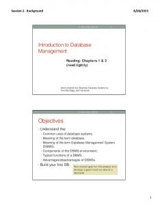
xii PREFACE 5. Native Macintosh Support:  LINGO's user interface has been entirely rewritten to offer native support for the Macintosh. Below is an image of the Mac version running a small nonlinear program. Notice the syntax highlighting, etc:

6. GUI Interface for Linux Versions of Lingo:  In the past, Linux versions had a command-line interface, as opposed to the easier to use GUI interface found on Windows versions. Linux versions of LINGO now have a full GUI interface similar to the Windows version's interface. 7. Matrix Functions:  There have been a number of new functions were added to LINGO for performing matrix operations. Supported operations include: eigenvalues and eigenvector computation, matrix determinant, Cholesky factorization, matrix inverse, and matrix transpose. 8. Linear Regression:  The new @REGRESS function for multiple linear regression has been added.

PREFACE

xiii

9. Other Improvements:  Tornado charts now supported.  Additional sorting capabilities, convenient for data preparation and solution reporting.  A new date function, @STM2YMD, for converting LINGO's standard time values into the equivalent calendar date and time. We hope you enjoy this new release of LINGO. Many of the new features in this release are due to suggestions from our users. In particular, we'd like to thank both Robert Coughlan and Wu Jian (Jack) for their many useful suggestions for improving LINGO. If there are any features you'd like to see in the next release of LINGO, please let us know. Feel free to reach us at: LINDO Systems Inc. 1415 N. Dayton St. Chicago, Illinois 60642 (312) 988-7422 [email protected] http://www.lindo.com

April 2016

1 Getting Started with LINGO LINGO is a simple tool for utilizing the power of linear and nonlinear optimization to formulate large problems concisely, solve them, and analyze the solution. Optimization helps you find the answer that yields the best result; attains the highest profit, output, or happiness; or the one that achieves the lowest cost, waste, or discomfort. Often these problems involve making the most efficient use of your resources-including money, time, machinery, staff, inventory, and more. Optimization problems are often classified as linear or nonlinear, depending on whether the relationships in the problem are linear with respect to the variables. If you are a new user, it is recommended you go through the first seven chapters of this document to familiarize yourself with LINGO. Then you may want to see On Mathematical Modeling for more information on the difference between linear and nonlinear models and how to develop large models. It may also be helpful to view some sample models in Developing More Advanced Models or Additional Examples of LINGO Modeling to see if a particular template example is similar to a problem you have. For users of previous versions of LINGO, the new features are summarized in the Preface at the beginning of the manual.

Getting Started on Windows Installing LINGO on Windows Installing the LINGO software is straightforward. To setup LINGO for Windows, place your CD in the appropriate drive and run the installation program SETUP contained in the LINGO folder. Alternatively, if you downloaded LINGO from the LINDO website, locate the download installation program and double-click it to run the installation. The LINGO installation program will open and guide you through the steps required to install LINGO on your hard drive. Note:

If there is a previous version of LINGO installed on your machine, then you may need to uninstall it before you can install the new copy of LINGO. To uninstall the existing copy of LINGO, click on the Windows Start button, select the Settings command, select Control Panel, then double-click on the Add or Remove Programs icon. You should then be able to select LINGO and have the old version removed from your system.

2 CHAPTER 1

Starting LINGO on Windows Once LINGO is installed, you will find a new Lingo icon on your desktop:

You may double-click on the icon to start LINGO. Once LINGO is running, your screen will resemble the following:

The outer window labeled LINGO is the main frame window. All other windows will be contained within this window. The top of the frame window also contains all the command menus and the command toolbar. See Menu Commands for details on the toolbar and menu commands. The lower edge of the main frame window contains a status bar that provides various pieces of information

GETTING STARTED

3

regarding LINGO's current state. Both the toolbar and the status bar can be suppressed through the use of the Options command. The smaller child window labeled LINGO Model - LINGO1 is a new, blank model window. In the next section, we will be entering a sample model directly into this window. Many copies of LINGO come with their licenses pre-installed. However, some versions of LINGO require you to input a license key. If your version of LINGO requires a license key, you will be presented with the following dialog box when you start LINGO:

Your license key may have been included in an email sent to you when you ordered your software. The license key is a string of letters, symbols and numbers, separated into groups of four by hyphens (e.g., r82m-XCW2-dZu?-%72S-fD?S-Wp@). Carefully enter the license into the edit field, including hyphens. License keys are case sensitive, so you must be sure to preserve the case of the individual letters when entering your key. Click the OK button and, assuming the key was entered correctly, LINGO will then start. In the future, you will be able to run LINGO directly without entering the key. Note:

If you received your license key by email, then you have the option of cutting-and-pasting it into the license key dialog box. Cut the key from the email that contains it with the Ctrl+C key, then select the key field in LINGO dialog box and paste the key with the Ctrl+V key.

4 CHAPTER 1 If you don’t have a key, you can choose to run LINGO in demo mode by clicking the Demo button. In demo mode, LINGO has all the functionality of a standard version of LINGO with the one exception that the maximum problem size is restricted. Demo licenses expire after 180 days.

Opening a Sample Model on Windows LINGO is shipped with a directory containing many sample models. These models are drawn from a wide array of application areas. For a complete listing of these models, see Additional Examples of LINGO Modeling. The sample model directory is titled Samples and is stored directly off the many LINGO directory. To open a sample model in LINGO, follow these steps: 1. Pull down the File menu and select the Open command. You should see the following dialog box:

GETTING STARTED

5

2. Double-click on the folder titled Samples contained in the main LINGO folder installed off your root folder, at which point you should see:

6 CHAPTER 1 3. To read in a small transportation model, type Tran in the File Name field in the above dialog box and press the Open button. You should now have the model in an open window in LINGO as follows:

For details on developing a transportation model in LINGO see The Problem in Words in Getting Started with LINGO.

GETTING STARTED You may now solve the model using the Solver|Solve command or by pressing the button on the toolbar. The optimal objective value for this model is 161. When solved, you should see the following solver status window:

Note the objective field has a value of 161 as expected. For an interpretation of the other fields in this window, see Solver Status Window in Getting Started with LINGO.

7

8 CHAPTER 1 Behind the solver status window, you will find the solution report for the model. This report contains summary information about the model as well as values for all the variables. This report’s header is reproduced below:

For information on interpreting the fields in the solution report, see Sample Solution Report in Getting Started with LINGO.

GETTING STARTED

9

Getting Started on a Mac Installing LINGO on a Mac LINGO for the Mac is distributed as a .DMG file, or disk image file, titled LINGO-OSX-64x86-16.0.dmg. If you double-click on this file you should see a window similar to the following:

To install LINGO onto your Mac, drag the LINGO icon in the window to the Applications folder icon. This will place a copy of LINGO in the /Applications folder of your hard drive. The Mac version of LINGO requires that you have installed OS X 10.7, or later, on your system.

10 CHAPTER 1 We also recommend that you drag a copy of the LingoDocs folder in the above window to your hard drive. The LingoDocs folder contains copies of LINGO's sample models and documentation. You may want to place this folder in your $HOME folder (subsequent documentation will assume this is the case).

Starting LINGO on a Mac Once LINGO is installed, you will find a new LINGO icon in the /Applications folder on your Mac's hard drive. The icon should appear as follows:

GETTING STARTED

11

You may double-click on the icon to start LINGO. Once LINGO is running, your screen will resemble the following:

The outer window is the main frame window, and all other windows will be contained within this main frame window. The top of the main frame window also contains a toolbar for executing various LINGO commands. The smaller child window labeled Lingo Model - Lingo1.lng is a new, blank model window. In the Developing a LINGO Model section, we will be entering a sample model directly into this window.

12 CHAPTER 1 Unlike the Windows version of LINGO, the command menus do not appear at the top of the main frame window, but appear in the Finder's menu bar whenever LINGO is the active application. Below, we see the six LINGO menus — Lingo, File, Edit, Solver, Window and Help — in the Finder's menu bar at the top of the screen:

See the LINGO Commands section for details on the toolbar and menu commands. The lower edge of the main frame window contains a status bar that provides various pieces of information regarding LINGO's current state. Both the toolbar and the status bar can be suppressed through the LINGO|Preferences command.

GETTING STARTED

13

Many copies of LINGO come with their licenses pre-installed. However, some versions of LINGO require you to input a license key. If your version of LINGO requires a license key, you will be presented with the following dialog box when you start LINGO:

Your license key may have been included in an email sent to you when you ordered your software. The license key is a string of letters, symbols and numbers, separated into groups of four by hyphens (e.g., r82m-XCW2-dZu?-%72S-fD?S-Wp@). Carefully enter the license into the edit field, including hyphens. License keys are case sensitive, so you must be sure to preserve the case of the individual letters when entering your key. Click the OK button and, assuming the key was entered correctly, LINGO will then start. In the future, you will be able to run LINGO directly without entering the key. Note:

If you received your license key by email, then you have the option of copying-and-pasting it into the license key dialog box. Copy the key from the email with the Command+C key, then select the key field in LINGO dialog box and paste the key with the Command+V key.


Opening a Sample Model on a Mac In the Installing LINGO on a Mac section above, we suggested that you install the LingoDocs folder in your $HOME directory. The LingoDocs folder contains a folder called Samples with numerous sample model. These models are drawn from a wide array of application areas. For a complete listing of these models, see Additional Examples of LINGO Modeling. The sample model directory is titled Samples and is stored directly off the main LINGO directory. To open a sample model in LINGO, follow these steps: 1.

Pull down the File menu and select the Open command. Migrate to where you installed your copy of the LingoDocs folder:

GETTING STARTED

2.

Double-click on the LingoDocs folder then double-click on the Samples folder contained in the LingoDocs folder, at which point you should see:

15

16 CHAPTER 1 3.

To read in a small transportation model, select the tran.lng model from the Sample folder and press the Open button. You should now have the model in an open window in LINGO as follows:

GETTING STARTED

17

18 CHAPTER 1 For details on developing a transportation model in LINGO see The Problem in Words in Getting Started with LINGO. You may now solve the model using the Solver|Solve command, or by pressing the Solve button on the toolbar:

The optimal objective value for this model is 161. When solved, you should see the following solver status window:


GETTING STARTED

19

Behind the solver status window, you will find the solution report for the model. This report contains summary information about the model as well as values for all the variables. This report’s header is reproduced below:


20 CHAPTER 1

Features Not Currently Supported on the Mac The Mac version of LINGO is a new addition and currently doesn't support the entire feature set found under Windows. The currently unsupported features are listed below:    

Excel interface ODBC database connectivity Callable LINGO API @USER user supplied function

We encourage you to check back at www.lindo.com frequently to see if any of these features have become available on Mac LINGO.

Getting Started on Linux Installing LINGO on Linux Linux versions of LINGO are distributed as a Run file, titled LINGO-LINUX-64x86-16.0.run, which is an automated installation program that will do the work required to set up LINGO on your Linux machine. Once you've copied this file onto your machine, you should first set the file's protections so that it is executable. You may do this by opening a Linux terminal window, changing to the directory with the Run file, and entering the command: chmod 755 ./LINGO-LINUX-64x86-16.0.run -v

You may then start the install program by entering: ./LINGO-LINUX-64x86-16.0.run

If you are installing LINGO with normal user rights, the install program defaults to putting LINGO in your $HOME/lingo16 folder. If your LINGO license permits multiple users, then you can install LINGO as a super user, in which case, LINGO defaults to installing in the /opt/lingo16 folder, where it may be accessed by other users on the machine. In either case, the default location may be changed to suit your needs.

GETTING STARTED

21

Starting LINGO on Linux Once LINGO is installed, a new LINGO icon will appear on your desktop. The icon should appear as follows:

You may double-click on the icon to start LINGO.

22 CHAPTER 1 Once LINGO is running, your screen will resemble the following:

The outer window is the main frame window, and all other windows will be contained within this main frame window. The top of the main frame window also contains a toolbar for executing various LINGO commands. The smaller child window labeled Lingo Model - Lingo1.lng is a new, blank model window. In the Developing a LINGO Model section, we will be entering a sample model directly into this window. See the Menu Commands section for details on the toolbar and menu commands. The lower edge of the main frame window contains a status bar that provides various pieces of information regarding LINGO's current state. Both the toolbar and the status bar can be suppressed through the Solver|Options command.

GETTING STARTED

23

Many copies of LINGO come with their licenses pre-installed. However, some versions of LINGO require you to input a license key. If your version of LINGO requires a license key, you will be presented with the following dialog box when you start LINGO:

Your license key may have been included in an email sent to you when you ordered your software. The license key is a string of letters, symbols and numbers, separated into groups of four by hyphens (e.g., r82m-XCW2-dZu?-%72S-fD?S-Wp@). Carefully enter the license into the edit field, including hyphens. License keys are case sensitive, so you must be sure to preserve the case of the individual letters when entering your key. Click the OK button and, assuming the key was entered correctly, LINGO will then start. In the future, you will be able to run LINGO directly without entering the key. Note: If you received your license key by email, then you have the option of copying-and-pasting it into the license key dialog box. Copy the key from the email with the Ctrl+C key, then select the key field in LINGO dialog box and paste the key with the Ctrl+V key.


Opening a Sample Model on Linux LINGO's installation program also copies a number of sample LINGO models onto your hard drive. These models can be found in the samples folder, immediately beneath the main lingo16 folder. In most cases, the folder containing the samples will be $HOME/lingo16/samples. These models are drawn from a wide array of application areas. For more discussion of these models, see Additional Examples of LINGO Modeling. To open a sample model in LINGO, follow these steps: 1. Pull down the File menu and select the Open command. You will be presented with the following file selection dialog, and it will be open to the samples folder:

GETTING STARTED

25

2. Double-click on the LingoDocs folder then double-click on the Samples folder contained in the LingoDocs folder, at which point you should see:

26 CHAPTER 1 3. To read in a small transportation model, select the tran.lng model from the samples folder and press the Open button. You should now have the model in an open window in LINGO as follows:

GETTING STARTED

27

For details on developing a transportation model in LINGO see The Problem in Words in Getting Started with LINGO. You may now solve the model using the Solver|Solve command, or by pressing the Solve button on the toolbar: . The optimal objective value for this model is 161. When solved, you should see the following solver status window:


28 CHAPTER 1 Behind the solver status window, you will find the solution report for the model. This report contains summary information about the model as well as values for all the variables. This report’s header is reproduced below:


GETTING STARTED

29

Features Not Currently Supported on Linux The Linux version of LINGO is a new addition and currently doesn't support the entire feature set found under Windows. The currently unsupported features are listed below:   

Excel interface ODBC database connectivity @USER user supplied function

We encourage you to check back at www.lindo.com frequently to see if any of these features have become available on the Linux version of LINGO.

Command-Line Prompt On machines other than Windows, Mac and Linux, you may have to interface with LINGO through the means of a command-line prompt. All instructions are issued to LINGO in the form of text command strings. When you start a command-line version of LINGO, you will see a colon command prompt as follows: LINGO Copyright (C) LINDO Systems Inc. Licensed material, all rights reserved. Copying except as authorized in license agreement is prohibited. :

The colon character (:) at the bottom of the screen in LINGO’s prompt for input. When you see the colon prompt, LINGO is expecting a command. When you see the question mark prompt, you have already initiated a command and LINGO is asking you to supply additional information related to this command such as a number or a name. If you wish to "back out" of a command you have already started, you may enter a blank line in response to the question mark prompt and LINGO will return you to the command level colon prompt. All available commands are listed in Command-line Commands.

Entering the Model from the Command-Line When you enter a model in the command-line interface, you must first specify to LINGO that you are ready to begin entering the LINGO statements. This is done by entering the MODEL: command at the colon prompt. LINGO will then give you a question mark prompt and you begin entering the model line by line.

30 CHAPTER 1 As an example, we will use the CompuQuick model discussed in the previous section. After entering the CompuQuick model, your screen should resemble the following (note that user input is in bold): : ? ? ? ? ? :

MODEL: MAX = 100 * STANDARD + 150 * TURBO; STANDARD =3; = DEMAND( J)); ! The supply constraints; @FOR( WAREHOUSE( I): [SUP] @SUM( CUSTOMER( J): VOLUME( I, J)) = 100; 10] @FOR(THINGS: @BIN(X)); : !Change the direction of the constraint : ALTER 9 '>='0: number of bins)

122

SPBIGM

1.E8

Scaling warning threshold

SP sampling random number seed

Max scenarios allowed in an SP before auto sampling takes effect

Stochastic solver Big M coefficient

Command-Line Commands 373 123

NSLPSV

0

Use SLP solver for nonlinear models (0:no, 1:yes)

124

FORCEB

0

Enforce variable bounds in calc and data sections (0:no, 1:yes)

125

NTHRDS

1

Max number of executions threads (0:use all cores, 1:single-threaded, N>1:use up to N threads

126

MTMODE

0

Multithreading mode (-1:LINGO chooses, 0:off in solver,1:prefer parallel, 2:parallel exclusively, 3:prefer concurrent, 4:concurrent exclusively)

127

BNPBLK

2

Branch-and-price (BNP) blocks (0:use row names, 1:user specified, 2:off, >2:max number of blocks)

128

BNPHEU

1

BNP block-finding heuristic (1:GP1, 2:GP2)

129

REPROD

0

Favor reproducibility (0:no, 1:yes)

1. ILFTOL and 2. FLFTOL Due to the finite precision available for floating point operations on digital computers, LINGO can’t always satisfy each constraint exactly. Given this, LINGO uses these two tolerances as limits on the amount of violation allowed on a constraint while still considering it “satisfied”. These two tolerances are referred to as the initial linear feasibility tolerance (ILFTOL) and the final linear feasibility tolerance (FLFTOL). The default values for these tolerances are, respectively, 0.000003 and 0.0000001. ILFTOL is used when the solver first begins iterating. ILFTOL should be greater than FLFTOL. In the early stages of the solution process, being less concerned with accuracy can boost the performance of the solver. When LINGO thinks it has an optimal solution, it switches to the more restrictive FLFTOL. At this stage in the solution process, one wants a relatively high degree of accuracy. Thus, FLFTOL should be smaller than ILFTOL. One instance where these tolerances can be of use is when LINGO returns a solution that is almost, but not quite, feasible. You can verify this by checking the values in the Slack or Surplus column in the model’s solution report. If there are only a few rows with small, negative values in this column, then you have a solution that is close to being feasible. Loosening (i.e., increasing the values of) ILFTOL and FLFTOL may help you get a feasible solution. This is particularly true in a model where scaling is poor (i.e., very large and very small coefficients are used in the same model), and the units of measurement on some constraints are such that minor violations are insignificant. For instance, suppose you have a budget constraint measured in millions of dollars. In this case, a violation of a few pennies would be of no consequence. Short of the preferred method of rescaling your model, loosening the feasibility tolerances may be the most expedient way around a problem of this nature.

374 CHAPTER 6 3. INFTOL and 4. FNFTOL The initial nonlinear feasibility tolerance (INFTOL) and the final nonlinear feasibility tolerance (FNFTOL) are both used by the nonlinear solver in the same manner the initial linear and final linear feasibility tolerances are used by the linear solver. For information on how and why these tolerances are useful, refer to the section immediately above. Default values for these tolerances are, respectively, 0.001 and 0.000001. 5. RELINT RELINT, the relative integrality tolerance, is used by LINGO as a test for integrality in integer programming models. Due to round-off errors, the “integer” variables in a solution may not have values that are precisely integral. The relative integrality tolerance specifies the relative amount of violation from integrality that is acceptable. Specifically, if I is the closest integer value to X, X will be considered an integer if: |X - I| 0 X ∈ (0,1)

@PBETAINV( A, B, X)

Inverse Beta

A = alpha > 0 B = beta > 0 X ∈ [0,1]

@PBETAPDF( A, B, X)

Beta PDF

A = alpha > 0 B = beta > 0 X ∈ (0,1)

@PCACYCDF( L, S, X)

Cumulative Cauchy

@PCACYINV( L, S, X)

Inverse Cauchy

L = location S = scale > 0 X a real L = location S = scale > 0 X ∈ [0,1]

OPERATORS AND FUNCTIONS @PCACYPDF( L, S, X)

Cauchy PDF

@PCHISCDF( DF, X)

Cumulative Chi-Square

L = location S = scale > 0 X a real DF = degrees of freedom = a positive integer X≥ 0

@PCHISINV( DF, X)

Inverse Chi-Square

DF = degrees of freedom = a positive integer X ∈ [0,1]

@PCHISPDF( DF, X)

Chi-Square PDF

DF = degrees of freedom = a positive integer X≥ 0

@PEXPOCDF( L, X)

Cumulative Exponential

L = lambda > 0 X≥ 0

@PEXPOINV( L, X)

Inverse Exponential

L = lambda > 0 X ∈ [0,1]

@PEXPOPDF( L, X)

Exponential PDF

L = lambda > 0 X≥ 0

@PFDSTCDF( DF1, DF2, X)

Cumulative F-Distribution

DF1,DF2 = degrees of freedom = a positive integer X≥ 0

@PFDSTINV( DF1, DF2, X)

Inverse F-Distribution

DF1,DF2 = degrees of freedom = a positive integer X ∈ [0,1]

@PFDSTPDF( DF1, DF2, X)

F-Distribution PDF

DF1,DF2 = degrees of freedom = a positive integer X≥ 0

@PGAMMCDF( SC, SH, X)

Cumulative Gamma

SC = scale > 0 SH = shape > 0 X≥ 0

@PGAMMINV( SC, SH, X)

Inverse Gamma

SC = scale > 0 SH = shape > 0 X ∈ [0,1]

@PGAMMPDF( SC, SH, X)

Gamma PDF

SC = scale > 0

441

442 CHAPTER 7 SH = shape > 0 X≥ 0 @PGMBLCDF( L, S, X)

Cumulative Gumbel

@PGMBLINV( L, S, X)

Inverse Gumbel

L = location S = scale > 0 X a real L = location S = scale > 0 X ∈ [0,1]

@PGMBLPDF( L, S, X)

Gumbel PDF

@PLAPLCDF( L, S, X)

Cumulative Laplace

@PLAPLINV( L, S, X)

Inverse Laplace

L = location S = scale > 0 X a real L = location S = scale > 0 X a real L = location S = scale > 0 X ∈ [0,1]

@PLAPLPDF( L, S, X)

Laplace PDF

@PLGSTCDF( L, S, X)

Cumulative Logistic

@PLGSTINV( L, S, X)

Inverse Logistic

L = location S = scale > 0 X a real L = location S = scale > 0 X a real L = location S = scale > 0 X ∈ [0,1]

@PLGSTPDF( L, S, X)

Logistic PDF

@PLOGNCDF( M, S, X)

Cumulative Lognormal

@PLOGNINV( M, S, X)

Inverse Lognormal

L = location S = scale > 0 X a real M = mu S = sigma > 0 X>0 M = mu S = sigma > 0 X ∈ [0,1]

@PLOGNPDF( M, S, X)

Lognormal PDF

M = mu

OPERATORS AND FUNCTIONS

@PNORMCDF( M, S, X)

Cumulative Normal

@PNORMINV( M, S, X)

Inverse Normal

S = sigma > 0 X>0 M = mu S = sigma > 0 X a real M = mu S = sigma > 0 X ∈ [0,1]

@PNORMPDF( M, S, X)

Normal PDF

@PPRTOCDF( SC, SH, X)

Cumulative Pareto

M = mu S = sigma > 0 X a real SC = scale > 0 SH = shape > 0 X ≥ SC

@PPRTOINV( SC, SH, X)

Inverse Pareto


@PPRTOPDF( SC, SH, X)

Pareto PDF

SC = scale > 0 SH = shape > 0 X ≥ SC

@PSMSTCDF( A, X)

Cumulative Symmetric Stable

A = alpha  [0.2,2] X a real

@PSMSTINV( A, X)

Inverse Symmetric Stable

A = alpha  [0.2,2] X  [0,1]

@PSMSTPDF( A, X)

Symmetric Stable PDF

@PSTUTCDF( DF, X)

Cumulative Student's t

@PSTUTINV( DF, X)

Inverse Student's t

A = alpha  [0.2,2] X a real DF = degrees of freedom = a positive integer X a real DF = degrees of freedom = a positive integer X ∈ [0,1]

@PSTUTPDF( DF, X)

Student's t PDF

DF = degrees of freedom = a positive integer X a real

443

444 CHAPTER 7 @PTRIACDF( L, U, M, X)

Cumulative Triangular

L = lower limit U = upper limit M = mode X ∈ [L,U]

@PTRIAINV( L, U, M, X)

Inverse Triangular

L = lower limit U = upper limit M = mode X ∈ [0,1]

@PTRIAPDF( L, U, M, X)

Triangular PDF

L = lower limit U = upper limit M = mode X ∈ [L,U]

@PUNIFCDF( L, U, X)

Cumulative Uniform

L = lower limit U = upper limit X ∈ [L,U]

@PUNIFINV( L, U, X)

Inverse Uniform

L = lower limit U = upper limit X ∈ [0,1]

@PUNIFPDF( L, U, X)

Uniform PDF

L = lower limit U = upper limit X ∈ [L,U]

@PWEIBCDF( SC, SH, X)

Cumulative Weibull


@PWEIBINV( SC, SH, X)

Inverse Weibull


@PWEIBPDF( SC, SH, X)

Weibull PDF


OPERATORS AND FUNCTIONS Discrete Distribution Functions

Description

Parameters

@PBTBNCDF( N, A, B, X)

Cumulative Beta Binomial

N = trials ∈ {0,1,...} A = alpha ∈ (0,+inf) B = beta ∈ (0,+inf) X ∈ [0, +inf)

@PBTBNINV( N, A, B, X)

Beta Binomial Inverse

N = trials ∈ {0,1,...} A = alpha ∈ (0,+inf) B = beta ∈ (0,+inf) X ∈ [0,+inf)

@PBTBNPDF( N, A, B, X)

Beta Binomial PDF

N = trials ∈ {0,1,...} A = alpha ∈ (0,+inf) B = beta ∈ (0,+inf) X ∈ [0,+inf)

@PBINOCDF( N, P, X)

Cumulative Binomial

N = trials ∈ {0,1,...} P = probability of success ∈ [0,1] X ∈ {0,1,...,N}

@PBINOINV( N, P, X)

Inverse Binomial

N = trials ∈ {0,1,...} P = probability of success ∈ [0,1] X ∈ [0,1]

@PBINOPDF( N, P, X)

Binomial PDF

N = trials ∈ {0,1,...} P = probability of success ∈ [0,1] X ∈ {0,1,...,N}

@PGEOMCDF( P, X)

Cumulative Geometric

P = probability of success ∈ (0,1] X ∈ {0,1,...}

@PGEOMINV( P, X)

Inverse Geometric

P = probability of success ∈ (0,1]

445

446 CHAPTER 7 X ∈ [0,1] @PGEOMPDF( P, X)

Geometric PDF

P = probability of success∈ (0,1] X ∈ {0,1,...}

@PHYPGCDF( N, D, K, X)

Cumulative Hypergeometric

N = population ∈ {0,1,...} D = number defective ∈ {0,1,...,N} K = sample size ∈ {0,1,...,N} X ∈ {max(0,D+KN),...,min(D,K)}

@PHYPGINV( N, D, K, X)

Inverse Hypergeometric

N = population ∈ {0,1,...} D = number defective ∈ {0,1,...,N} K = sample size ∈ {0,1,...,N} X ∈ [0,1]

@PHYPGPDF( N, D, K, X)

Hypergeometric PDF

N = population ∈ {0,1,...} D = number defective ∈ {0,1,...,N} K = sample size ∈ {0,1,...,N} X ∈ {max(0,D+KN),...,min(D,K)}

@PLOGRCDF( P, X)

@PLOGRINV( P, X)

Cumulative Logarithmic

P = p-factor ∈ (0,1)

Inverse Logarithmic

P = p-factor ∈ (0,1)

X ∈ {0,1,...,N} X ∈ [0,1]

@PLOGRPDF( P, X)

Logarithmic PDF

P = p-factor ∈ (0,1) X ∈ {0,1,...,N}

@PNEGBCDF( R, P, X)

Cumulative Negative Binomial

R = number of failures ∈ (0,+inf) P = probability of success ∈ (0,1) X ∈ {0,1,...}

OPERATORS AND FUNCTIONS @PNEGBINV( R, P, X)

Inverse Negative Binomial

447

R = number of failures ∈ (0,+inf) P = probability of success ∈ (0,1) X ∈ [0,1]

@PNEGBPDF( R, P, X)

Negative Binomial PDF

R = number of failures ∈ (0,+inf) P = probability of success ∈ (0,1) X ∈ {0,1,...}

@PPOISCDF( L, X)

Cumulative Poisson

L = lambda ∈ (0,+inf) X ∈ {0,1,...,N}

@PPOISINV( L, X)

Inverse Poisson

L = lambda ∈ (0,+inf) X ∈ [0,1]

@PPOISPDF( L, X)

Poisson PDF

L = lambda ∈ (0,+inf) X ∈ {0,1,...,N}

Report Functions Report functions are used to construct reports based on a model’s results, and are valid on both calc and data sections. Combining report functions with interface functions in a data section allows you to export the reports to text files, spreadsheets, databases, or your own calling application. Note:

The interested reader will find an exhaustive example of the use of report functions in the sample model TRANSOL.LG4 in the Samples subfolder. This model makes extensive use of many of the report functions to mimic the standard LINGO solution report.

@DUAL ( variable_or_row_name) The @DUAL function outputs the dual value of a variable or a row. For example, consider a model with the following data section: DATA: @TEXT( 'C:\RESULTS\OUTPUT.TXT') = @WRITEFOR( SET1( I): X( I), @DUAL( X( I)), @NEWLINE(1)); ENDDATA

448 CHAPTER 7 When this model is solved, the values of attribute X and their reduced costs will be written to the file C:\RESULTS\OUTPUT.TXT. Output may be routed to a file, spreadsheet, database or memory location. The exact destination will depend on the export function used on the left-hand side of the output statement. If the argument to the @DUAL function is a row name, then the dual price on the generated row will be output. @FORMAT ( value, format_descriptor) @FORMAT may be used in @WRITE and @WRITEFOR statements to format a numeric or string value for output as text, where value is the numeric or string value to be formatted, and format_descriptor is a string detailing how the number is to be formatted. The format descriptor is interpreted using C programming conventions. For instance, a format descriptor of ‘12.2f’ would cause a numeric value to be printed in a field of 12 characters with 2 digits after the decimal point. For a string values, such as a set member name, a format descriptor of '12s' would cause the string to be right justified in a field of 12 characters, while '-12s' would cause the string to be left justified in a field of 12. You can refer to a C reference manual for more details on the available formatting options. The following example uses the @FORMAT function to place a shipping quantity into a field of eight characters with no trailing decimal value: DATA: @TEXT() = @WRITE( ' From To Quantity', @NEWLINE(1)); @TEXT() = @WRITE( '--------------------------', @NEWLINE(1)); @TEXT() = @WRITEFOR( ROUTES( I, J) | X( I, J) #GT# 0: 3*' ', WAREHOUSE( I), 4*' ', CUSTOMER( J), 4*' ', @FORMAT( X( I, J), '8.0f'), @NEWLINE( 1)); ENDDATA

The report will resemble the following: From To Quantity -------------------------WH1 C1 2 WH1 C2 17 WH1 C3 1 WH2 C1 13 WH2 C4 12 WH3 C3 21

OPERATORS AND FUNCTIONS This next example, GRAPHPSN.LG4, graphs the standard normal function, @PSN, over the interval [ –2.4, 2.4]. The @FORMAT function is used to print the X coordinates with one trailing decimal point. ! Graphs @PSN() over a specified interval around 0; DATA: ! height of graph; H = 49; ! width of graph; W = 56; ! interval around 0; R = 2.4; ENDDATA SETS: S1 /1..H/: X, FX; ENDSETS @FOR( S1( I): ! X can be negative; @FREE( X); ! Compute x coordinate; X( I) = -R + ( I - 1)* 2 * R / ( H - 1); ! Compute y coordinate = @psn( x); FX( I) = @PSN( X( I)); ); DATA: ! Print the header; @TEXT() = @WRITE( 'Graph of @PSN() on the interval [-', R,',+',R,']:',@NEWLINE(1)); @TEXT() = @WRITE( '| 0 ',(W/2-5)*'-', ' 0.5 ',(W/2-5)*'-', '1.0 X(i)',@NEWLINE(1)); ! Loop to print the graph over; @TEXT() = @WRITEFOR( S1( I): '| ', ( W * FX( I) + 1/2) * '*', @IF( X( I) #LT# 0, '', ' '), ( W ( W * FX( I) + 1/2) + 3)*' ', @FORMAT( X(I), '.1f'),@NEWLINE(1)); !Trailer; @TEXT() = @WRITE( '| 0 ',(W/2-5)*'-', ' 0.5 ',(W/2-5)*'-', '1.0',@NEWLINE(1)); ENDDATA

Model: GRAPHPSN

449

450 CHAPTER 7 Here is how the graph will appear when the model is solved: Graph of @PSN() on the interval [-2.4,+2.4]: | 0 ----------------------- 0.5 -----------------------1.0 | | * | * | * | * | ** | ** | ** | *** | **** | ***** | ***** | ****** | ******** | ********* | ********** | ************ | ************** | *************** | ***************** | ******************* | ********************* | ************************ | ************************** | **************************** | ****************************** | ******************************** | *********************************** | ************************************* | *************************************** | ***************************************** | ****************************************** | ******************************************** | ********************************************** | *********************************************** | ************************************************ | ************************************************** | *************************************************** | *************************************************** | **************************************************** | ***************************************************** | ****************************************************** | ****************************************************** | ****************************************************** | ******************************************************* | ******************************************************* | ******************************************************* | ******************************************************* | ******************************************************** | 0 ----------------------- 0.5 -----------------------1.0

X(i) -2.4 -2.3 -2.2 -2.1 -2.0 -1.9 -1.8 -1.7 -1.6 -1.5 -1.4 -1.3 -1.2 -1.1 -1.0 -0.9 -0.8 -0.7 -0.6 -0.5 -0.4 -0.3 -0.2 -0.1 0.0 0.1 0.2 0.3 0.4 0.5 0.6 0.7 0.8 0.9 1.0 1.1 1.2 1.3 1.4 1.5 1.6 1.7 1.8 1.9 2.0 2.1 2.2 2.3 2.4


451

@ITERS () The @ITERS function returns the total number of iterations required to solve the model. @ITERS is available only in the data and calc sections, and is not allowed in the constraints of a model. For example, the following output statement writes the iteration count to the standard output device: DATA: @TEXT() = @WRITE('Iterations= ', @ITERS()); ENDDATA

@NAME ( var_or_row_reference) Use @NAME to return the name of a variable or row as text. @NAME is available only in the data and calc sections, and is not allowed in the constraints of a mode. The following example prints a variable name and its value: DATA: @TEXT() = @WRITEFOR( ROUTES( I, J) | X( I, J) #GT# 0: @NAME( X), ' ', X( I, J), @NEWLINE(1)); ENDDATA

The report will resemble the following: X( X( X( X( X( X(

WH1, WH1, WH1, WH2, WH2, WH3,

C1) C2) C3) C1) C4) C3)

2 17 1 13 12 21

@NEWLINE ( n) Use @NEWLINE to write n new lines to the output device. @NEWLINE is available only in the data and calc sections, and is not allowed in the constraints of a model. See the example immediately below in the @RANGED section. @OBJBND () @OBJBND returns the bound on the objective value. @RANGED ( variable_or_row_name) @RANGED outputs the allowable decrease on a specified variable’s objective coefficient or on a specified row’s right-hand side. @RANGED is available only in the data and calc sections, and is not allowed in the constraints of a model. For example, consider a model with the following data section: DATA: @TEXT( 'C:\RESULTS\OUTPUT.TXT') = @WRITEFOR( SET( I): X( I), @RANGED( X( I), @NEWLINE(1)); ENDDATA

452 CHAPTER 7 When this model is solved, the values of attribute X and the allowable decreases on its objective coefficients will be written to the file C:\RESULTS\OUTPUT.TXT. If @RANGED is passed a row name it will output the allowable decrease on the right-hand side value for the row. Output may be routed to a file, spreadsheet, database, or memory location. The exact destination will depend on the export function used on the left-hand side of the output statement. Range computations must be enabled in order for @RANGED to function properly. For more information on the interpretation of allowable decreases, refer to the Solver|Range command. @RANGEU ( variable_or_row_name) @RANGEU outputs the allowable increase on a specified variable’s objective coefficient or on a specified row’s right-hand side. For example, consider a model with the following data section: DATA: @TEXT( 'C:\RESULTS\OUTPUT.TXT') = @WRITEFOR( SET( I): X, @RANGEU(X), @NEWLINE(1)); ENDDATA

When this model is solved, the values of X and the allowable increases on its objective coefficients will be written to the file C:\RESULTS\OUTPUT.TXT. If @RANGEU is passed a row name it will output the allowable increase on the right-hand side value for the row. Output may be routed to a file, spreadsheet, database, or memory location. The exact destination will depend on the export function used on the left-hand side of the output statement. Range computations must be enabled in order for @RANGED to function properly. For more information on the interpretation of allowable increases, refer to the Solver|Range command.

OPERATORS AND FUNCTIONS @STATUS () This returns the final status of the solution process using the following codes: @STATUS() Code

Interpretation

0

Global Optimum — The optimal solution has been found.

1

Infeasible — No solution exists that satisfies all constraints.

2

Unbounded — The objective can be improved without bound.

3

Undetermined — The solution process failed.

4

Feasible — A feasible solution was found that may, or may not, be the optimal solution.

5

Infeasible or Unbounded — The preprocessor determined the model is either infeasible or unbounded. If you need to narrow the result down to either infeasible or unbounded, then you will need to turn off presolving and run the model again.

6

Local Optimum — Although a better solution may exist, a locally optimal solution has been found.

7

Locally Infeasible — Although feasible solutions may exist, LINGO was not able to find one.

8

Cutoff — The objective cutoff level was achieved.

9

Numeric Error — The solver stopped due to an undefined arithmetic operation in one of the constraints.

In general, if @STATUS does not return a code of 0, 4, 6 or 8, the solution is of little use and should not be trusted. The @STATUS function is available only in the data and calc sections. The @STATUS function is not allowed in the constraints of a model.

453

454 CHAPTER 7 For example, the following output statement uses @STATUS to print a message to let the user know if the solution is globally optimal, or not: DATA: @TEXT() = @WRITE( @IF( @STATUS() #EQ# 0, 'Global solution found', 'WARNING: Solution *not* globally optimal!'); ENDDATA

For additional examples of the use of the @STATUS function, refer to Interfacing with Other Applications. @STRLEN( string) Use @STRLEN to get the length of a specified string. This can be a useful feature when formatting reports. As an example, @STRLEN( ‘123’) would return the value 3. @STRLEN is available only in the data and calc sections, and is not allowed in the constraints of a model. @TABLE( ‘attr|set’) The @TABLE function is used to display either an attribute’s values or a set’s members in tabular format. The @TABLE function is available only in the data and calc sections of a model. You can refer to either QUEENS8.LG4 or PERT.LG4 for examples of @TABLE. These models can be found in the SAMPLES folder off the main LINGO folder. For instance, QUEENS8.LG4 is a model for positioning eight queens on a chessboard so that no one queen can attack another. At the end of this model you will find the following data section: DATA: @TEXT() = ' The final chessboard:'; @TEXT() = @TABLE( X); ENDDATA

Here we are using the @TABLE function to display the X attribute in the standard output window via the @TEXT interface function (see below for more on @TEXT). The X attribute is an 8-by-8 table of 0’s and 1’s indicating if a queen is positioned in a given square of the chessboard, or not. The output generated by @TABLE in this instance follows: The final chessboard: E1 E2 E3 E4 E5 E1 0 1 0 0 0 E2 0 0 0 0 1 E3 0 0 0 0 0 E4 0 0 0 1 0 E5 1 0 0 0 0 E6 0 0 0 0 0 E7 0 0 0 0 0 E8 0 0 1 0 0

E6 0 0 0 0 0 0 1 0

E7 0 0 1 0 0 0 0 0

E8 0 0 0 0 0 1 0 0

Note that all eight queens (indicated by the 1’s on the board) are safe from attack.


455

In addition to displaying attributes, @TABLE can also display sets. When displaying a set, @TABLE will print the letter X in the table cell if the corresponding set member exists, otherwise it will leave the table cell blank. The PERT.LG4 sample model is a project scheduling model. A project consists of many tasks, and some tasks must be completed before others can begin. The list of all the tasks that must precede certain other tasks is called the precedence relations. At the end of PERT4.LG4 there is the following data section which uses @TABLE to display the precedence relations set, PRED: DATA: !Use @TABLE() to display the precedence relations set, PRED; @TEXT() = @TABLE( PRED); ENDDATA When we run the model, @TABLE displays the following table: DESIGN FORECAST SURVEY PRICE SCHEDULE COSTOUT TRAIN DESIGN FORECAST SURVEY PRICE X SCHEDULE COSTOUT X TRAIN

X

X X X

X

X

Whenever one task must precede another, an ‘X’ appears in the particular cell of the table. So, for instance, the DESIGN task must precede the FORECAST and SURVEY tasks. If a line of a table exceeds the page width setting in Lingo, it simply gets wrapped around. So, if you want to display wide tables without line wraps, you may need to increase the page width. Note:

Currently, @TABLE can only send tables to the standard solution window or to text files. In other words, it is not possible to send tables to Excel, databases or to applications calling the LINGO DLL.

456 CHAPTER 7 @TABLE can also display sets and attributes of more than two dimensions. In fact, @TABLE allows you great control over how multidimensional objects get displayed. Specifically, four forms of @TABLE are supported: 

@TABLE( attr/set) – This is the simplest form of @TABLE. If the object is of one dimension, it will be displayed as a column. Otherwise, the first n-1 dimensions will be displayed on the vertical axis, while the n-th dimension will be displayed on the horizontal axis of the table. An example follows: @TABLE( X)



@TABLE( attr/set, num_horz_indices) – In this form, a second argument, num_horz_indices, is supplied. This argument is an integer quantity equal to the number of the object’s dimensions to display along the horizontal axis. In which case, dimensions (n – num_horz_indices) to n will be displayed along the horizontal axis of the table. The following example displays dimension 2 and 3 of a 3dimensional set along the horizontal axis: @TABLE( MY_3_DIM_SET, 2)



@TABLE( attr/set, prim_set1,...,prim_setn) – Here we specify the exact ordering of the object’s n dimensions. In which case, the first n-1 dimensions specified will be displayed along the vertical axis, while the last dimension specified will be displayed along the horizontal axis. Here’s an example that displays a 4-dimensional attribute with dimensions 3, 4 and 1 on the vertical, and dimension 2 on the horizontal: @TABLE( MY_4_DIM_ATTRIBUTE, 3, 4, 1, 2)



@TABLE( attr/set, prim_set1,...,prim_setn, num_horz_indices) – In this final form, we again specify the ordering of all the indices, but a final integer argument is added to specify the number of dimensions to be displayed on the horizontal axis. The following example displays a 4-dimensional attribute with dimensions 3 and 4 on the vertical, and dimensions 1 and 2 on the horizontal: @TABLE( MY_4_DIM_ATTRIBUTE, 3, 4, 1, 2, 2)

@WRITE(obj1[, …, objn]) Use @WRITE to output one or more objects. @WRITE is available only in the data and calc sections, and is not allowed in the constraints of a model. In a data section, output from @WRITE may be routed to a file, spreadsheet, or database. The exact destination will depend on the interface function used on the left-hand side of the output statement. @WRITE may also be used to display computations that are a function of variable values. As an example, the output statement below prints the ratio of the two variables X and Y: DATA: @TEXT() = @WRITE( 'The ratio of X to Y is: ', X / Y); ENDDATA


457

@WRITEFOR ( setname[ ( set_index_list) [ | cond_qualifier]]: obj1[, …, objn]) Use @WRITEFOR to output one or more objects across a set. @WRITEFOR is available only in the data and calc sections, and is not allowed in the constraints of a model @WRITEFOR operates like the other set looping functions in that you may, or may not, specify an index list and a conditional qualifier. The ability to use a conditional qualifier allows great flexibility in specifying exactly what you wish to display in your reports. @WRITEFOR may also be used to display computations that are a function of variable values. Using @WRITEFOR in conjunction with export functions in data sections allows you to route output to a file, spreadsheet, or database. The exact destination will depend on the export function used on the left-hand side of the output statement. As an example, the output statement below prints the number of units to ship, the warehouse name, and the customer name for each route with nonzero volume: DATA: @TEXT() = @WRITEFOR( ROUTES( I, J) | X( I, J) #GT# 0: 'Ship ', X( I, J), ' units from warehouse ', WAREHOUSE( I), ' to customer ', CUSTOMER( J), @NEWLINE( 1)); ENDDATA

The resulting report would appear as follows: Ship Ship Ship Ship Ship Ship

2 units from warehouse WH1 to customer C1 17 units from warehouse WH1 to customer C2 1 units from warehouse WH1 to customer C3 13 units from warehouse WH2 to customer C1 12 units from warehouse WH2 to customer C4 21 units from warehouse WH3 to customer C3

Text Replication Operator (*) The text replication operator (*) may be used inside either the @WRITE or @WRITEFFOR functions to repeat a string a specified number of times. The operator should be preceded by a numeric value and then followed by a string (e.g., 3*’text’), which will cause the string to be printed n times, where n is the numeric value. In the following example, the text replication operator is used twice to produce a simple graph of onduty staff during the seven days of the week: DATA: LEAD = 3; @TEXT() = 'Staff on duty graph:'; @TEXT() = @WRITEFOR( DAY( D): LEAD*' ', DAY( D), ' ', ON_DUTY( D), ' ', ON_DUTY( D)*'+', @NEWLINE(1) ); ENDDATA

458 CHAPTER 7 The graph would appear as follows, with one plus sign displayed for each staff member on duty: Staff on duty graph: MON 20 ++++++++++++++++++++ TUE 16 ++++++++++++++++ WED 12 ++++++++++++ THU 16 ++++++++++++++++ FRI 19 +++++++++++++++++++ SAT 14 ++++++++++++++ SUN 13 +++++++++++++

Date, Time and Calendar Functions @TIME() The @TIME function returns the total runtime, in seconds, required so far to generate and solve the model. @TIME is available only in the data and calc sections, and is not allowed in the constraints of a model. For example, the following output statement writes the solution time to the standard output device: CALC: @WRITE('Solve time in seconds =', @TIME()); ENDCALC

@YMD2STM( year, month, day, hour, minute, second) The @YMD2STM function takes a date and time as input and returns the equivalent scalar time, where scalar time is the number of seconds since the start of the base date of 1 Jan 2000. Note that dates prior to 1 Jan 2000 will return negative scalar time values. The first five arguments must be integral values, while the number of seconds can be fractional. If the seconds value is fractional, it will be rounded to the nearest 10 microseconds (or .00001 seconds). Hours are reported using military time and can range from 0 to 23. An example follows: CALC: !Convert two dates to scalar time; STM1 = @YMD2STM( 2013, 1, 24, 13, 30, 10.5); STM2 = @YMD2STM( 1787, 9, 17, 0, 0, 0); ENDCALC

Here, we compute the scalar time for the two dates and times: 1/23/2013 13:30:10.5 and 9/17/1787 00:00:00. The solution report lists the following values: Variable STM1 STM2

Value 412349410.50 -6699196800.0

There are two things to note: First, STM1 has a fractional value of .5, given that its time includes .5 fractional seconds. Second, STM2 is negative reflecting the fact that its date if prior to the base date to 1 Jan 2000.


459

YEAR, MON, DAY, DAYOFWEEK, HOUR, MIN, SEC = @STM2YMD( stm) The @STM2YMD function takes a standard time value and returns the year, month, day of month, day of week (Sunday being day 1), hour, minute and second. Any of the left-hand side arguments may be omitted if they are not of interest. Below, we pass the current standard time via @STMNOW (see below) to @STM2YMD and then display the results: MODEL: SETS: MONTHS / JAN..DEC/; DAYS / SUN..SAT/; ENDSETS CALC: ! Convert the current standard time to human readable form; YR, MN, DAY, DWK, HR, MI, SE = @STM2YMD( @STMNOW()); @WRITE( ' Year: ' Month: ' Day: 'Day of week: ' Hour: ' Minute: ' Second: ); ENDCALC

', ', ', ', ', ', ',

YR, @NEWLINE( 1), MONTHS( MN), @NEWLINE( 1), DAY, @NEWLINE( 1), DAYS( DWK), @NEWLINE( 1), HR, @NEWLINE( 1), MI, @NEWLINE( 1), SE, @NEWLINE( 2)

END

The output from the model shows the current date and time: Year: 2016 Month: FEB Day: 11 Day of week: THU Hour: 9 Minute: 14 Second: 36.427

The @STM2YMD function may be used in calc sections only and may not be used in the optimizable sections of a model.

460 CHAPTER 7 @STM2YR( stm) / @STM2MON( stm) / @STM2DAY( stm) @STM2HR( stm) / @STM2MIN( stm) / @STM2SEC( stm) These six functions are the inverses of the @STM2YR function presented above. Each function takes a scalar time value as input and returns, respectively, the year, month, day, hour, minute or second of the point in time represented by the scalar time value. Note that @STM2SEC can return fractional seconds. The following example takes a date and time, converts it to scalar time, and then converts the scalar time back to the original date and time: SETS: MONTHS /JAN..DEC/; DAYS /SUN..SAT/; ENDSETS CALC: !Convert a date to scalar time; STM = @YMD2STM( 1787, 9, 17, 12, 0, 0); !Convert the scalar time back to the original date and time; YR = @STM2YR( STM); MO = @STM2MON( STM); DA = @STM2DAY( STM); HR = @STM2HR( STM); MN = @STM2MIN( STM); SC = @STM2SEC( STM); DOW = @STM2DWK( STM); !Write out the original date; @WRITE( 'Date: ', DA, ' ', MONTHS( MO), ' ', YR, @NEWLINE( 1); ); !And the original date; @WRITE( 'Time: ', HR, ':', @FORMAT( MN, '%02g'), ':', @FORMAT( SC, '%02g'), @NEWLINE( 1); ); !And the day of the week; @WRITE( 'Day: ', DAYS( DOW), @NEWLINE( 2); ); ENDCALC


461

The output from this sample follows: Date: 17 SEP 1787 Time: 12:00:00 Day: MON

@STMNOW() The @STMNOW returns the current date and time as a scalar time value, where scalar time is the number of seconds since the base date of 1 Jan 2000. The returned may be fractional to indicate fractions of a second. The returned value can be broken down into the corresponding year, month, day, hour, minute and second by calling the @STM2* inverse functions described above. An example for displaying the current date and time follows: MODEL: SETS: MONTHS /JAN..DEC/; DAYS /SUN..SAT/; ENDSETS CALC: T = @STMNOW(); YR = @STM2YR( T); MO = @STM2MON( T); DA = @STM2DAY( T); HR = @STM2HR( T); MN = @STM2MIN( T); SC = @STM2SEC( T); DWK = @STM2DWK( T); @SET( 'TERSEO', 1); @WRITE( ' The current date and time is:', ' ', DAYS( DWK), ' ', DA, ' ', MONTHS( MO), ' ', YR, ', ', HR, ':', @FORMAT( MN, '%02g'), ':', @FORMAT( SC, '%04.1f'), @NEWLINE( 2) ); ENDCALC END

462 CHAPTER 7 Here, we retrieve the current date and time as a scalar time value using @STMNOW. We then convert the scalar time to a calendar date and time and then write out the result. The following is a sample of output from the model: The current date and time is: MON 11 FEB 2013, 15:54:56.7

@STM2DWK( stm) The @STM2DWK function takes a scalar time and returns the index of its day of the week, with Sunday returning 1 and Saturday returning 7. An example of @STM2DWK can be found immediately above.

Matrix Functions Matrix functions take one or more matrices (or attributes) as arguments. Unlike most other LINGO functions, which primarily return scalar (or single-value) results, some matrix functions can return multiple results, with some of the results being matrices or vectors. Matrix functions supported are:      

Cholesky factorization, Matrix determinants, Eigenvalues and eigenvectors, Matrix inversion, Multiple linear regression, and Matrix transpose.

Note :

All matrix functions are only supported in calc sections of models. At present, matrix functions are not valid inside model (optimizable) sections.

Note:

All matrix functions work entirely with dense matrices. Matrices defined on sparse sets are not supported.

L[, err] = @CHOLESKY( A) The @CHOLESKY function performs a Cholesky factorization of the symmetric, positive-definite matrix A, where LL' = A, and L is a lower-triangular matrix with real and positive diagonal elements. One can think of L as the "square root" of matrix A. Both A and L must be square and of the same dimension. The upper triangle of L will be filled with zeros. The optional argument, err, is an error flag that will be 0 if the factorization was successful, otherwise it will be 1. If err is present, any error will be ignored by LINGO and will be left for your model to handle. If err is not present, then, on any error, LINGO will display an error message and terminate the run.


463

In this example below, we take a small 3x3 matrix, A, compute its Cholesky factor, L, then show that LL' is equal to the original matrix A. MODEL: ! ! ! !

Compute the Cholesky factorization of matrix A. Back check by taking the Cholesky factor, L, and multiplying it with its transpose, L', to get the original matrix A;

SETS: S1; S2(S1,S1): A, A2, L, LT; ENDSET DATA: S1 = 1..3; A = 10 11 12 11 54 51 12 51 86; ENDDATA CALC: ! Get the Cholesky factor; L = @CHOLESKY( A); ! L transpose; LT = @TRANSPOSE( L); ! Compute L * L'; @FOR( S2( I, J): A2( I, J) = @SUM( S1( J2): L( I, J2) * LT( J2, J)); ); ENDCALC CALC: @SET( 'TERSEO', 2) ; ! Just display errors; @WRITE( "Original A matrix:", @NEWLINE( 1)); @TABLE( A); @WRITE( @NEWLINE( 1), "Cholesky factor L:", @NEWLINE( 1)); @TABLE( L); @WRITE( @NEWLINE( 1), "L transpose:", @NEWLINE( 1)); @TABLE( LT); @WRITE( @NEWLINE( 1), "L * L' = A:", @NEWLINE( 1)); @TABLE( A2); ENDCALC END

Model: CHOLESKY

464 CHAPTER 7 The output from this model is reproduced below, where we can see, as per definition, LL' = A: Original A matrix 1 2 1 10.00000 11.00000 2 11.00000 54.00000 3 12.00000 51.00000

3 12.00000 51.00000 86.00000

Cholesky factor L: 1 2 1 3.162278 0.000000 2 3.478505 6.473021 3 3.794733 5.839623

3 0.000000 0.000000 6.123627

L transpose: 1 1 3.162278 2 0.000000 3 0.000000

2 3.478505 6.473021 0.000000

3 3.794733 5.839623 6.123627

2 11.00000 54.00000 51.00000

3 12.00000 51.00000 86.00000

L * L' = A: 1 2 3

1 10.00000 11.00000 12.00000

@DETERMINANT( A) The @DETERMINANT function returns the determinant value for matrix A. In the example below, we make use of Cramer's Rule for finding the solution to a system of linear equations of the form Ax=b. According to Cramer's Rule, the solution for x( i) may be calculated by computing the determinant of the A matrix with column i replaced by the right-hand side values b. This determinant value is then divided by the determinant of the original A matrix to get the final value for x( i).

OPERATORS AND FUNCTIONS MODEL: ! Use Cramer's Rule to find the solution to a system of linear equations, Ax=b; SETS: DIM: X, B, B2; DXD( DIM, DIM): A, A2; ENDSETS DATA: DIM = 1..3; B = 12 0 -3; A = 1 -2 5 4 1 -2 -2 1 -1 ; ENDDATA CALC: ! Determinant of the original matrix; D = @DETERMINANT( A); ! Determine if a unique solution exists; @IFC( D #EQ# 0: @STOP( ' No unique solution exists!!!'); @ELSE @WRITE( ' A unique solution exists...'); ); @WRITE( @NEWLINE( 1)); ! Copy matrix; @FOR( DXD( I, J): A2( I, J) = A( I, J)); @FOR( DIM( J): ! Replace column J with the B values; @FOR( DIM( I): A2( I, J) = B( I); ); ! Calculate solution for X( J); X( J) = @DETERMINANT( A2) / D; ! Restore column J in the original matrix; @FOR( DIM( I): A2( I, J) = A( I, J); ); ); ! Back check the solution;

465

466 CHAPTER 7 @FOR( DIM( I): B2( I) = @SUM( DIM( J): A( I, J) * X( J)); @IFC( @ABS( B2( I) - B( I)) #GT# 1.E-6: @STOP( 'Solution fails!!!!'); ); ); @WRITE( ' Solution verified...', @NEWLINE( 1), ' Solution = '); @FOR( DIM( I): @WRITE( X( I), '

'));

@WRITE( @NEWLINE( 2)); ENDCALC END

Model: CRAMER We first checked to see if a unique solution to the system exists by computing the determinant of the original matrix and checking that it was not 0. We then used Cramer's Rule to compute the solution vector, x. Finally, we took the x values and verified that they solve the equations. The output from the model is: A unique solution exists... Solution verified... Solution = 1 2 3

LAMDAR, VR, LAMBDAI, VI, ERR = @EIGEN( A) The @EIGEN function returns eigenvectors and eigenvalues for the matrix A, where:  A  LAMBDAR  VR  LAMBDAI  VI  err

a nxn matrix, a vector of length n for returning the real parts of the eigenvalues, a nxn matrix for returning the real parts of the eigenvectors (one vector per column), a vector of length n for returning the imaginary parts of the eigenvalues, a nxn matrix for returning the imaginary parts of the eigenvectors, and an error flag that will be 1 if a numeric problem occurs, otherwise 0.

As long as at least one left-hand side argument is present, all other arguments may be omitted. If err is present, then LINGO will not halt the run if a numeric error occurs; it will be up to your model to handle the error. If err is not present and a numeric error occurs, then LINGO will halt model execution. In the next example, we compute the eigenvalues and eigenvectors for a 3x3 symmetric matrix.

OPERATORS AND FUNCTIONS MODEL: SETS: DIM: LAMBDA; DXD( DIM, DIM): A, V, AV, LV; DXDL( DXD) | &1 #GT# &2: PROD; ENDSETS DATA: TOL = 1.E-6; DIM = 1..3; A = 3 4 1 4 0 9 1 9 5; ENDDATA CALC: ! Compute the eigenvalues and eigen vectors; ! Note: The matrix is symmetric, so the vectors ! and values will not have imaginary parts, so ! we can omit the imaginary arguments.; LAMBDA, V,,, ERR = @EIGEN( A); ! Numeric error?; @IFC( ERR #NE# 0: @STOP( 'Numeric error')); ! Display them with the @TABLE function.; @WRITE( @NEWLINE( 1), ' Eigenvalues:', @NEWLINE( 2)); @TABLE( LAMBDA); @WRITE( @NEWLINE( 1), ' Eigenvectors:', @NEWLINE( 1)); @TABLE( V); ! Check that A * v = Lambda * v holds.; NZ = 0; @FOR( DXD( I, J): LV( I, J) = LAMBDA( J) * V( I, J); AV( I, J) = @SUM( DIM( K): A( I, K) * V( K, J)); @IFC( @ABS( LV( I, J) - AV( I, J)) #GT# TOL: NZ = NZ + 1); ); @WRITE( @NEWLINE( 1)); @IFC( NZ #GT# 0: @WRITE( ' Lambda * v = A * v is not verified.'); @ELSE @WRITE( ' Lambda * v = A * v is verified.'); ); ! Symmetric matrices have orthogonal eigenvectors. ! Verify this by computing the inner products.;

467

468 CHAPTER 7 NZ = 0; @FOR( DXDL( I, J): PROD( I, J) = @sum( DIM( K): V( K, I) * V( K, J)); @IFC( @ABS( PROD( I, J)) #GT# TOL: NZ = NZ + 1); ); @WRITE( @NEWLINE( 1)); @IFC( NZ #GT# 0: @WRITE( ' Eigenvectors are NOT orthogonal.', @NEWLINE( 2)); @ELSE @WRITE( ' Eigenvectors are orthogonal.', @NEWLINE( 2)); ); ENDCALC END

Model: EIGENEX1 Symmetric matrices have the property that their eigenvalues and eigenvectors are all real valued, allowing us to ignore the imaginary components. Looking at the call to @EIGEN: LAMBDA, V,,, ERR = @EIGEN( A);

we see that two left-hand side arguments are omitted, corresponding to the imaginary parts. Note, we could have passed these two arguments, however, they would have simply been filled with all zeros. By the definition of eigenvalues and eigenvectors, it's true that Av = Lambda * v, where A is the original nxn matrix, v is an nx1 eigenvector of A, and Lambda is the eigenvalue corresponding to v. The model verifies this relationship and displays the message: Lambda * v = A * v is verified.

Another nice property of symmetric matrices is that the eigenvectors are all orthogonal. The model verifies this property by calculating all the inner products between the eigenvectors and comparing these products to 0. The output from the model follows: Eigenvalues: 1 2 3

12.92039 2.587500 -7.507889

Eigenvectors: 1 2 3

1 -0.3179176 -0.6062189 -0.7289904

2 -0.9145159 -0.6813624E-02 0.4044926

Lambda * v = A * v is verified. Eigenvectors are orthogonal.

3 0.2501781 -0.7952686 0.5522307


469

AINV[, err] = @INVERSE( A) The @INVERSE function returns the inverse of matrix A. Both AINV and A must be square, nxn matrices. The optional argument, err, is an error flag that will be 0 if the invert operation was successful, otherwise it will be 1. A situation where err would be nonzero is when A is a singular matrix. If err is present, any error will be ignored by LINGO and will be left for your model to handle. If err is not present, then, on any error, LINGO will display an error message and terminate the run. The example below may be familiar from the @DETERMINANT example above, where we solve a 3x3 system of linear equations. In this example, however, we will not use Cramer's Rule to solve the system. Instead, we will compute the inverse of the A matrix, and then multiply the inverse by the right-hand side vector b to get the solution vector x. We also verify that a unique solution exists by computing the determinant of A, as well as verify that our solution does indeed solve the original set of equations.

470 CHAPTER 7 MODEL: SETS: DIM: X, B, B2; DXD( DIM, DIM): A, AINV; ENDSETS DATA: DIM = 1..3; B = 12 0 -3; A = 1 -2 5 4 1 -2 -2 1 -1 ; ENDDATA CALC: ! Determinant of the original matrix; D = @DETERMINANT( A); ! Determine if a unique solution exists; @IFC( D #EQ# 0: @STOP( ' No unique solution exists!!!'); @ELSE @WRITE( ' A unique solution exists...'); ); @WRITE( @NEWLINE( 1)); ! Get the matrix inverse; AINV = @INVERSE( A); ! Use the inverse to compute the solution vector: x = AINV * b; @FOR( DIM( I): X( I) = @SUM( DIM( J): AINV( I, J) * B( J))); ! Back check the solution; @FOR( DIM( I): B2( I) = @SUM( DIM( J): A( I, J) * X( J)); @IFC( @ABS( B2( I) - B( I)) #GT# 1.E-6: @STOP( 'Solution fails!!!!'); ); ); @WRITE( ' Solution verified...', @NEWLINE( 1), ' Solution = '); @FOR( DIM( I): @WRITE( @FORMAT( X( I), '10.5g'))); @WRITE( @NEWLINE( 2)); ENDCALC END

Model: INVERSE


471

The output from the model follows: A unique solution exists... Solution verified... Solution = 1

2

3

Again, as with the @DETERMINANT example, the solution is [1,2,3]. B, b0, RES, rsq, f, p, var = @REGRESS( Y, X) The @REGRESS function is used to perform multiple linear regression (MLR), a technique that models the linear relationship, Y = b0 + B*X, between one dependent variable and one or more independent variables. MLR is frequently used in forecasting, e.g., by economists in macroeconomics when modeling of the economy. Using the syntax above, we have the following definitions: B  b0  RES  rsq

f P  var Y X

The vector of coefficient terms for the regression. If there are p independent variables, then B is a vector of length p. The constant term of the regression. If a constant term is not desired, then you can omit this argument and LINGO will force the constant term to 0. The residuals, or error terms. These are the differences between the predicted and actual observed values for the dependent variable. The R-squared statistic, a measure of strength of the relationship between the model and dependent variable. The fraction of the original variance removed by the forecast formula versus using just b0 alone. The F-value, a measure of the overall significance of the model. The p-value for the regression, a measure of the significance of the F-test. Estimate of variance of the residual terms. The observed values for the dependent variable. If there are n observations, then Y should be a vector of length n. The independent variable values. If there are n observations and p independent variables, then X should be an nxp matrix.

Note, that any of the left-hand side arguments may be omitted if they are not of interest. The only requirement is that at least one left-hand side argument must be present. The goal of MLR is to fit a linear function to the observed data, X, for predicting the independent observations, Y. The form of the function is: Y = b0 + ∑ i B( i) * X( i) + RES The fit is determined by the set of coefficients that minimizes the sum of the squared residual values. For more information, see: https://en.wikipedia.org/wiki/Line.

472 CHAPTER 7 In the LINGO sample models folder, there is a regression example called REGRLONG, shown below. This model makes use of the Longley dataset: http://www.itl.nist.gov/div898/strd/lls/data/LINKS/DATA/Longley.dat This is a series of seven macroeconomic statistics, with one being total employment, the dependent variable. The Longley dataset is commonly used for testing statistical software, and the link above contains the certified results for regressions based on the data.

OPERATORS AND FUNCTIONS MODEL: ! Multiple linear regression; ! The output is the set of regression coefficients, B, for the model: Y(i) = B(0) + B(1)*X(i,1) + B(2)*X(i,2)+... + ERROR(i) We use the Longley macroeconomic data set for: http://www.itl.nist.gov/div898/strd/lls/data/LINKS/DATA/Longley.dat Certified Regression Statistics for Longley data: Parameter B(0) B(1) B(2) B(3) B(4) B(5) B(6)

Estimate -3482258.63459582 15.0618722713733 -0.358191792925910E-01 -2.02022980381683 -1.03322686717359 -0.511041056535807E-01 1829.15146461355

Residual Standard Deviation

304.854073561965

R-Squared

0.995479004577296

Standard Deviation of Estimate 890420.383607373 84.9149257747669 0.334910077722432E-01 0.488399681651699 0.214274163161675 0.226073200069370 455.478499142212

Certified Analysis of Variance Table: Source of Variation Regression Residual

Degrees of Sums of Freedom Squares 6 184172401.944494 9 836424.055505915

Mean Squares 30695400.3240823 92936.0061673238

F Statistic 330.285339234588 ; SETS: OBS : Y, RES; VARS; DEPVAR( VARS); ! The dependent variable; EXPVAR( VARS): B; ! The explanatory variables; OXV( OBS, VARS): DATATAB; ! The data table; OXE( OBS, EXPVAR): X; ENDSETS DATA: ! Names of the variables; VARS = EMPLD PRICE GNP__ JOBLS MILIT POPLN

YEAR_;

473

474 CHAPTER 7 ! Dependent variable. Must be exactly 1; DEPVAR = EMPLD; ! Explanatory variables. Should not include dependent variable; EXPVAR = PRICE GNP__ JOBLS MILIT POPLN YEAR_; ! The dataset; DATATAB = 60323 83 61122 88.5 60171 88.2 61187 89.5 63221 96.2 63639 98.1 64989 99 63761 100 66019 101.2 67857 104.6 68169 108.4 66513 110.8 68655 112.6 69564 114.2 69331 115.7 70551 116.9

234289 259426 258054 284599 328975 346999 365385 363112 397469 419180 442769 444546 482704 502601 518173 554894

2356 2325 3682 3351 2099 1932 1870 3578 2904 2822 2936 4681 3813 3931 4806 4007

1590 1456 1616 1650 3099 3594 3547 3350 3048 2857 2798 2637 2552 2514 2572 2827

107608 108632 109773 110929 112075 113270 115094 116219 117388 118734 120445 121950 123366 125368 127852 130081

1947 1948 1949 1950 1951 1952 1953 1954 1955 1956 1957 1958 1959 1960 1961 1962;

ENDDATA CALC: !Suppress some of Lingo's output; @SET( 'TERSEO', 2); !Set up data for the @REGRESS function by moving the dependent variable into Y and the independents into X; @FOR( DEPVAR( K): @FOR( OBS( I): Y( I) = DATATAB( I, K); @FOR( OXE( I, J): X( I, J) = DATATAB( I, J)) ); ); ! Do the regression; B, B0, RES, RSQUARE, F, P, VAR = @REGRESS( Y, X); ! Print a @WRITE( ' @FORMAT( @WRITE( ' @FORMAT( @WRITE( ' @FORMAT( @WRITE( '

report; Explained error/R-Square: ', RSQUARE, '16.8g'), @NEWLINE(1)); F statistic: ', F, '16.8g'), @NEWLINE(1)); p value: ', P, '16.8g'), @NEWLINE(1)); Residual variance: ',


475

@FORMAT( VAR, '16.8g'), @NEWLINE(1)); @WRITE( ' Residual std error: ', @FORMAT( VAR ^ .5, '16.8g'), @NEWLINE(2)); @WRITE( ' B( 0): ', @FORMAT( B0, '16.8g'), @NEWLINE( 1)); @FOR( EXPVAR( I): @WRITE( ' B( ', EXPVAR( I), '): ', @FORMAT( B( I), '16.8g'), @NEWLINE( 1)); ); ENDCALC END

Model: REGRLONG The interesting parts of this model are the following two expressions: !Set up data for the @REGRESS function by moving the dependent variable into Y and the independents into X; @FOR( OBS( I): Y( I) = DATATAB( I, @INDEX( EMPLD)); @FOR( OXE( I, J): X( I, J) = DATATAB( I, J)) ); ! Do the regression; B, B0, RES, RSQUARE, F, P, VAR = @REGRESS( Y, X);

Note, that the data is provided as a single table, containing both the dependent and independent observations. The first expression partitions the raw data into a vector Y of dependent employment observations, and a 16x6 X matrix of independent observations. At this point, the data is in the correct format to submit to @REGRESS, and we perform the regression with the statement: ! Do the regression; B, B0, RES, RSQUARE, F, P, VAR = @REGRESS( Y, X);

Results from the regression are then displayed: Explained error/R-Square: F statistic: p value: Residual variance: Residual std error: B( B( B( B( B( B( B(

0): PRICE): GNP__): JOBLS): MILIT): POPLN): YEAR_):

-3482258.6 15.061872 -0.035819179 -2.0202298 -1.0332269 -0.051104106 1829.1515

0.995479 330.28534 4.984031e-010 92936.006 304.85407

476 CHAPTER 7 T = @TRANSPOSE( A) The @TRANSPOSE function returns the transpose of matrix A, where T(i,j) = A(j,i) for every (i,j). Matrix A does not have to be square, but if A is an mxn matrix, then T must be of dimension nxm. For an example of @TRANSPOSE, refer to the section above on @CHOLESKY, where we use @TRANSPOSE to get the transpose of the Cholesky factor. This transpose is then multiplied by the original Cholesky factor to get the original matrix back.

Miscellaneous Functions @BLOCKROW( block_index, row_name) The @BLOCKROW function is used in conjunction with the branch-and-price (BNP) solver. Models suited for BNP have 2 or more mostly independent subproblems known as blocks. @BLOCKROW is used to assign rows to their respective blocks, where block_index is the index of the block and row_name is the name of the row to assign to block block_index. Block indices may be any nonnegative, integer value, with 0 corresponding to the block of linking rows. Refer to the BNP Solver section in Chapter 5 for more information on the use of @BLOCKROW. @IF (logical_condition, true_result, false_result) The @IF function evaluates logical_condition and, if true, returns true_result. Otherwise, it returns false_result. For example, consider the following simple model that uses @IF to compute fixed production costs: MIN = COST; COST = XCOST +YCOST; XCOST = @IF( X #GT# 0, 100, 0) + 2 * X; YCOST = @IF( Y #GT# 0, 60, 0) + 3 * Y; X + Y >= 30;

Model: IFCOST We produce two products—X and Y. We want to minimize total cost, subject to producing at least 30 total units of X and Y. If we produce X, there is a fixed charge of 100 along with a variable cost of 2. Similarly, for Y, these respective values are 60 and 3. We use the @IF function to determine if either of the products are being produced in order to apply the relevant fixed cost. This is accomplished by testing to see if their production levels are greater than 0. If so, we return the fixed cost value. Otherwise, we return zero. Experienced modelers know that, without the benefit of an @IF function, modeling fixed costs requires invoking some “tricks” using binary integer variables. The resulting models are not as intuitive as models constructed using @IF. However, the caveat is that the @IF function is not a linear function. At best, the graph of an @IF function will be piecewise linear. In our current example, the @IF functions are piecewise linear with a discontinuous break at the origin. It is always best to try and keep a model linear (see Chapter 15, On Mathematical Modeling). Barring this, it is best for all functions in a nonlinear model to be continuous. The @IF function violates both these conditions. Thus, models containing @IF functions may be tough to solve to global optimality. Fortunately, LINGO has two options that can help overcome the difficult nature of models containing @IF functions—linearization and global optimization.


477

To illustrate the difficulty in solving models with discontinuous functions such as @IF, we will solve our example model with both linearization and global optimization disabled. When we do this, we get the following solution: Local optimal solution found at iteration: Objective value: 160.0000 Variable COST XCOST YCOST X Y

42

Value 160.0000 160.0000 0.000000 30.00000 0.000000

This solution involves producing only X at a total cost of 160. Given that producing only Y and not X will result in a lower total cost of 150, this is clearly a locally optimal point. In order to find the globally optimal point, we must resort to either the linearization or global optimization features in LINGO. Briefly, linearization seeks to reformulate a nonlinear model into a mathematically equivalent linear model. This is desirable for two reasons. First, linear models can always be solved to global optimality. Secondly, linear models will tend to solve much faster than equivalent nonlinear models. Unfortunately, linearization can not always transform a model into an equivalent linear state. In which case, it may be of no benefit. Fortunately, our sample model can be entirely linearized. To enable the linearization option, run the Solver|Options command and set the Linearization Degree to High on the General Solver tab. Global optimization breaks a model down into a series of smaller, local models. Once this series of local models has been solved, a globally optimal solution can be determined. To enable global optimization, run the Solver|Options command, select the Global Solver tab, then click on the Global Solver checkbox. Note that the global solver is an add-on option to LINGO. The global solver feature will not be enabled for some installations. Run the Help|About LINGO command to determine if your installation has the global solver capability enabled. Whether using the linearization option or the global solver, LINGO obtains the true, global solution: Global optimal solution found at iteration: Objective value: 150.0000 Variable COST XCOST YCOST X Y

Note:

6

Value 150.0000 0.000000 150.0000 0.000000 30.00000

Starting with release 9.0, the false branch of the @IF function may contain arithmetic errors without causing the solver to trigger an error. This makes the @IF function useful in avoiding problems when the solver strays into areas where certain functions become undefined. For instance, if your model involves division by a variable, you might use @IF as follows: @IF( X #GT# 1.E-10, 1/X, 1.E10).

478 CHAPTER 7 @WARN (‘text’, logical_condition) This displays the message ‘text’ if the logical_condition is met. This feature is useful for verifying the validity of a model’s data. In the following example, if the user has entered a negative interest rate, the message “INVALID INTEREST RATE” is displayed: ! A model of a home mortgage; DATA: ! Prompt the user for the interest rate, years, and value of mortgage. We will compute the monthly payment; YRATE = ?; YEARS = ?; LUMP = ?; ENDDATA ! Number of monthly payment; MONTHS = YEARS * 12; ! Monthly interest rate; (1 + MRATE) ^ 12 = 1 + YRATE; ! Solve next line for monthly payment; LUMP = PAYMENT * @FPA(MRATE, MONTHS); ! Warn them if interest rate is negative @WARN('INVALID INTEREST RATE', YRATE #LT# 0);

@USER (user_determined_arguments) The user can supply this in an external DLL or object code file. For a detailed example on the use of @USER, please see the User Defined Functions section in Chapter 11, Interfacing with Other Applications.

8 Interfacing with External Files It can be cumbersome and impractical to try to maintain your data in a LINGO model file. In most cases, your model’s data will reside externally in text files, spreadsheets, and databases. Also, a solution generated by LINGO is of little use if you can’t export it to other applications. For these reasons, LINGO has many methods to assist you in moving information in and out of the application. The primary focus of this chapter is to illustrate how to move data in and out of LINGO through the use of text based ASCII files. In Chapter 9, Interfacing with Spreadsheets, we will look at using spreadsheets. In Chapter 10, Interfacing with Databases, we will illustrate the use of databases for maintaining your model’s data.

Cut and Paste Transfers Perhaps the simplest and most straightforward way to move data in and out of an application in Windows is by using cut and paste commands. Windows maintains an information buffer called the clipboard. Applications that support the cut command can move information into the clipboard. Applications that support the paste command can move information from the clipboard into their memory. Thus, cut and paste offers a simple, but effective, technique for moving small amounts of data from one application to another.

Pasting in Data from Excel You should be able to paste data into LINGO from any application that supports a cut command. For illustration purposes, we will show how to paste data from an Excel worksheet into a LINGO model. Recall our staff-scheduling model from Chapter 2, Using Sets, which is reproduced here with the data for the REQUIRED attribute omitted from the data section: SETS: DAYS / MON TUE WED THU FRI SAT SUN/: REQUIRED, START; ENDSETS DATA: REQUIRED = ; ENDDATA MIN = @SUM(DAYS(I): START(I)); @FOR(DAYS(J): @SUM(DAYS(I) | I #LE# 5: START(@WRAP(J - I + 1, 7))) >= REQUIRED(J) );

480 CHAPTER 8 Suppose your staffing requirements data is maintained in an Excel worksheet resembling the following:

To paste the staffing requirements data from Excel into the LINGO model above, follow these steps: 1. 2. 3. 4. 5.

Select the range containing the data (C3:I3) by placing the cursor on the C3 cell, press and hold down the left mouse button, drag the mouse to cell I3, then release the mouse button. Select the Copy command from Excel’s Edit Menu. Click once on the LINGO model window. Place the LINGO cursor directly to the right of the data statement: REQUIRED =. Select the Paste command from LINGO’s Edit menu.

The data should now appear in the LINGO model as follows: DATA: REQUIRED = 20 16 13 16 19 14 12; ENDDATA

You may need to adjust the font of the data to your liking. You can use the Edit|Select Font command in LINGO to accomplish this. Your model now has the required data and is ready to be solved. Note that LINGO also has features that allow you to import data directly from Excel. See Chapter 9, Interfacing with Spreadsheets, for more information.

Pasting Data Out to Microsoft Word Suppose you went ahead and solved the previous staffing model. LINGO will present you with a new Window containing the solution to your model. Now, suppose you would like to get a copy of the solution into MS Word for a report you are writing. You can do this by following these steps: 1. 2. 3. 4. 5.

Select the solution report window in LINGO by clicking on it once. Select all the text in the window by issuing the Edit|Select All command in LINGO. Place the solution into the clipboard by selecting the Edit|Copy command in LINGO. Activate MS Word by clicking once on the window containing the report you are writing. Paste the solution from the clipboard into the report by issuing the Edit|Paste command in MS Word.

INTERFACING WITH EXTERNAL FILES

481

Text File Interface Functions LINGO has several interface functions that perform input and output operations. There are interface functions for dealing with text files, spreadsheets, and databases. There is even an interface function that lets you pass data back and forth from other applications. In this chapter, we are focusing on interfacing with text files, so we will investigate the @FILE function for importing the contents of external text files and the @TEXT function for exporting solutions to text files.

Including External Files with @FILE The @FILE interface function in LINGO allows you to include data from external text files anywhere in your model. This is particularly useful for incorporating data stored in text files into your sets and data sections. The syntax for the @FILE function is: @FILE(‘filename’) where filename is the name of the file to include text from. When this function is encountered in a model, LINGO will continue to take text from this file until it encounters either the end-of-file mark or a LINGO end-of-record mark (~). For subsequent @FILE references in the same model that use the same file name, LINGO resumes taking input from the file at the point where it left off. Nesting of @FILE function calls (embedding an @FILE in a file that is itself called by @FILE) is not allowed.

482 CHAPTER 8

Using @FILE in a Transportation Model As an example, we will use the Wireless Widgets transportation model developed in Chapter 1, Getting Started with LINGO. It is reproduced in its original form below: ! A 6 Warehouse 8 Vendor Transportation Problem; SETS: WAREHOUSES /WH1 WH2 WH3 WH4 WH5 WH6/: CAPACITY; VENDORS /V1 V2 V3 V4 V5 V6 V7 V8/ : DEMAND; LINKS(WAREHOUSES, VENDORS): COST, VOLUME; ENDSETS ! The objective; MIN = @SUM(LINKS(I, J): COST(I, J) * VOLUME(I, J)); ! The demand constraints; @FOR(VENDORS(J): @SUM(WAREHOUSES(I): VOLUME(I, J)) = DEMAND(J)); ! The capacity constraints; @FOR(WAREHOUSES(I): @SUM(VENDORS(J): VOLUME(I, J)) 0 in our new report: Global optimal solution found at iteration: Objective value: MON TUE THU FRI SAT

15 22.00000

8.0 2.0 6.0 3.0 3.0

Another feature of this last example to note is the use of the @FORMAT function, which we used to display the nonzero start values in a field of six columns with one trailing decimal point. @WRITEFOR also allows us to form arithmetic expressions of the variable values. Here's an example that we could add to our staff model to compute the number of staff on duty each day: DATA: @TEXT( ) = @WRITE( 'Day On-Duty'); @TEXT( ) = @WRITE( 14*'-'); @TEXT( ) = @WRITEFOR( DAYS( D): DAYS(D), @FORMAT( @SUM( DAYS( D2) | D2 #LE# 5: START( @WRAP( D - D2 + 1, 7))), '11.1f')); ENDDATA


489

Here's the report generated by these output operations: Day On-Duty -------------MON 20.0 TUE 16.0 WED 13.0 THU 16.0 FRI 19.0 SAT 14.0 SUN 12.0

This previous example also illustrates the use of the @WRITE function. The @WRITE function is similar to the @WRITEFOR function with the exception that it does not accept a set to loop on, and, therefore, is used to write single occurrences of text output. As with @WRITEFOR, @WRITE accepts expressions of variables. Here's an example that calculates the maximum number of employees starting on a particular day. DATA: @TEXT() = @WRITE( 'Max start = ', @MAX( DAYS: START)); ENDDATA

which yields the following output: Max start = 8.

LINGO Command Scripts A LINGO command script is any text file containing a series of LINGO commands. In addition to understanding the syntax of LINGO models, using command scripts requires some understanding of LINGO’s command language (covered in Chapter 6, Command-line Commands). You can think of these commands as a macro language that allows you to automate the running of frequently used commands and/or models. To run a command script in Windows versions of LINGO, use the File|Take Commands command. In other versions of LINGO, use the TAKE command. In both cases, you will be prompted for the name of a file that contains your command script. Once you have input the file name, LINGO will begin to execute the commands in this file. Execution will continue until either a QUIT command is encountered, causing LINGO to terminate, or an end-of-file is encountered, causing LINGO to return to normal input mode.

490 CHAPTER 8

A Command Script Example Once again, we will make use of the staff-scheduling model introduced on page 84 to illustrate the use of a command script. Suppose, instead of one hot dog stand, our operations have expanded and we now have three hot dog stands: Pluto Dogs, Mars Dogs, and Saturn Dogs. Our staffing requirements at the three sites are: Site Pluto Mars Saturn

Mon 20 10 8

Tue 16 12 12

Wed 13 10 16

Thu 16 11 16

Fri 19 14 18

Sat 14 16 22

Sun 12 8 19

Running staffing models for all three sites is cumbersome and prone to error. We would like to automate the process by constructing a script file that runs all three staffing models automatically. To do this, we construct the following script file: ! Have LINGO echo input to the screen; SET ECHOIN 1 ! Suppresses the standard solution report; SET TERSEO 1 ! Begins input of a new model; MODEL: SETS: DAYS / MON TUE WED THU FRI SAT SUN/: REQUIRED, START; ENDSETS DATA: REQUIRED = @FILE('PLUTO.LDT'); @TEXT('PLUTO.TXT') = START; ENDDATA MIN = @SUM(DAYS(I): START(I)); @FOR(DAYS(J): @SUM(DAYS(I) | I #LE# 5: START(@WRAP(J - I + 1, 7))) >= REQUIRED(J) ); @FOR(DAYS: @GIN(START)); END ! Solve Pluto Dogs model; GO ! Alter model for Mars; ALTER ALL 'PLUTO'MARS' ! Solve Mars model; GO ! Alter model for Saturn; ALTER ALL 'MARS'SATURN' ! Solve Saturn model; GO


491

! Restore parameters; SET TERSEO 0 SET ECHOIN 0

Command Script: DOGS.LTF We use two SET commands to set two of LINGO’s parameters. First, we set ECHOIN to 1, which causes LINGO to echo all command script input to the screen. This can be useful when you are trying to debug a script file. Next, we set TERSEO to 1. This causes LINGO to go into terse output mode, which suppresses the default solution report each time we solve a model. Next, we include the MODEL: command to put LINGO into model input mode. It is important here to remember the MODEL: statement is a command. When LINGO encounters this command in a script file, it reads all subsequent text in the file as model text until it encounters the END command. This model then becomes the current model in memory. The key feature to note in our model is the data section: DATA: REQUIRED = @FILE('PLUTO.LDT'); @TEXT('PLUTO.TXT') = START; ENDDATA

We use the @FILE function to include the staffing requirements from an external file and we use the @TEXT function to send the values of the START attribute to a file. After the END statement, we have a GO command to solve the model for the Pluto stand. We then include an ALTER command to change all occurrences of PLUTO with MARS. This command will change the data section to (changes in bold): DATA: REQUIRED = @FILE('MARS.LDT'); @TEXT('MARS.TXT') = START; ENDDATA

Assuming we have the staffing requirements for the Mars stand in the file MARS.LDT, our model is then ready to run again. However, this time it will solve for the START values for the Mars hot dog stand. We include commands to do the same for the Saturn location as well. Finally, we have two SET commands to restore the modified parameters. You can run this command script by issuing the File|Take Commands command in Windows versions of LINGO, or you can use the TAKE command in other versions. Once the command script has been executed, you will find the three solution files: PLUTO.TXT, MARS.TXT, and SATURN.TXT. These files will contain the optimal values for the START attribute for the three locations.

The AUTOLG.DAT Script File LINGO has an option that allows you to automatically execute a command script each time LINGO starts. To do this, simply name the command script AUTOLG.DAT and place it in LINGO’s working directory. Each time LINGO starts, it will automatically execute the commands in this script file.

492 CHAPTER 8

Specifying Files in the Command-line When a Windows version of LINGO starts up, it checks the command-line for the presence of the following three commands: Command -Tfilename -Ofilename -Lfilename

Action at Runtime LINGO executes a File|Take Commands command on the script file filename. If an AUTOLG.DAT file is present in LINGO’s working directory, it will be queued for execution before filename. LINGO performs a File|Open command on filename, reading the file into a standard window. LINGO executes a File|Log Output command, causing all output that would normally have been sent to the command window to be routed to filename.

As an example, suppose we have the following command script: ! Input a small model MODEL: MAX = 20 * X + 30 * Y; X output_file Upon execution of this command, LINGO will take its input from input_file, and a text file will be created called output_file, which contains everything that would have appeared on the screen had LINGO been started normally. Path names may be included in the names of the input and output files. Exploiting this capability allows you to use LINGO as a “black box” in larger turnkey applications. If done properly, the user will not be aware LINGO is running in the background. As an example, we could run the script file from the previous section, TEST.LTF, generating the same solution file, SOLU.TXT, with the command: LINGO < TEST.LTF > CAPTURE.TXT

The file CAPTURE.TXT is used to capture all screen output.

Managing LINGO Files In order to help keep track of your files, you may want to adopt a file naming standard, at least as far as the file name extensions are concerned. Here are some suggestions for file name extensions: Extension .LG4 .LNG .LTF .LDT .LGR

Description model files (Windows only) model files in text format script files included data files report files

498 CHAPTER 8 A Note to Windows Users: If you use the default LINGO format (.LG4) for a model, the file will be saved in a special binary format. Files in this format will only be readable by Windows versions of LINGO, and will appear garbled if read into other applications. This binary format allows LINGO models to function as both Object Linking and Embedding (OLE) containers and servers, allows for embedding of objects (e.g., bitmaps), and permits custom formatting of model text. Thus, you will generally want to use the .LG4 format. Cases where you must use a text format are: 1. a model that must be transferred to another platform or application, 2. a LINGO script file, or 3. a LINGO data file to be included with @FILE. LINGO anticipates this by saving any file with an extension other than .LG4 as text. You can force LINGO to always use the .LNG text format for models by checking the .LNG box on the Interface tab of the Solver|Options dialog box. Any special formatting of the text (e.g., bold fonts) will be lost when a model is saved in this format. Also, models saved as text may not function as OLE containers or servers. On platforms other than Windows, LINGO always saves files in text format.

9 Interfacing With Spreadsheets As we have mentioned, it can be cumbersome and impractical to try to maintain your data in a LINGO model file. This is particularly true if you have more than just a small handful of data—as is the case with most practical models. Spreadsheets are adept at handling small to moderate amounts of data. Spreadsheets are also very useful tools for manipulating and presenting the results generated by your model. For these reasons, LINGO has a number of features that allow the user to import data from spreadsheets and export solutions back out to spreadsheets. These features include real-time Object Linking and Embedding (OLE) links to Excel, OLE automation links that can be used to drive LINGO from Excel macros, and embedded OLE links that allow you to import the functionality of LINGO into Excel. At present, all of these features are supported only under Windows versions of LINGO.

Importing Data from Spreadsheets LINGO provides the @OLE function for importing data from spreadsheets. This function is only available under Windows versions of LINGO. @OLE performs direct OLE transfers of data between LINGO and Excel.

Using @OLE to Import Data from Excel @OLE is an interface function for moving data back and forth from Excel using OLE based transfers. OLE transfers are direct memory transfers and do not make use of intermediate files. When using @OLE, LINGO loads Excel, tells Excel to load the desired spreadsheet, and requests ranges of data from the sheet. You must have Excel 5, or later, to be able to use the @OLE function. The @OLE function may be used in the data and init sections to import data. @OLE can read both set members and set attributes—set members are expected in text format, while set attributes are expected in numeric format. Primitive sets require one cell of data for each set member (i.e., one set member per cell). You will need n cells of values to initialize each n-dimensional derived set member, where the first n cells contain the first set member, the second n cells contain the second set member, and so on. @OLE can read one or two-dimensional ranges (ranges on a single worksheet in Excel), but cannot read discontinuous ranges or three-dimensional ranges (ranges that traverse more than one worksheet in Excel). Ranges are read left-to-right, top-to-bottom.

500 CHAPTER 9

Importing in the Data and Init Sections with @OLE The syntax for using @OLE to import data in both the data and init sections is: object_list = @OLE([‘spreadsheet_file’] [, range_name_list]); The object_list is a list of model objects, optionally separated by commas, which are to be initialized from the spreadsheet. Object_list may contain any combination of set names, set attributes, and scalar variables. The spreadsheet_file is the name of the Excel spreadsheet file to retrieve the data from. If the name is omitted, LINGO defaults to using whatever workbook is currently open in Excel. The range_name_list is the list of named ranges in the sheet to retrieve the data from. The ranges must contain exactly one element for each member in the object_list. There are three options available in how you specify the ranges. First, you can omit the range arguments entirely. In which case, LINGO defaults to using a list of range names identical to the list of object names in object_list. Second, you can specify a single range name to retrieve all the data from. In which case, all the objects in object_list must be defined on the same set, and LINGO reads the data as if it was a table. When specifying a single range name for multiple objects, all the objects must be of the same data type. Furthermore, you can’t mix set members (text) with set attributes (numeric). Finally, you can specify one range name for each object in object_list. In which case, the objects do not have to be defined on the same set and can be of differing data types. Examples of these three methods for using @OLE follow: Example 1: COST, CAPACITY = @OLE(); In this example we specify no arguments to the @OLE() function. In which case, LINGO will supply the default arguments. Given that no workbook name was specified, LINGO will use whatever workbook is currently open and active in Excel. In addition, no range names were specified, so LINGO defaults to using the names of the model objects. Thus, COST and CAPACITY are initialized to the values found, respectively, in the ranges COST and CAPACITY in the currently open workbook in Excel. Note:

If you do not specify a workbook name in @OLE() function references, LINGO defaults to using whatever workbook is currently open in Excel. Therfore, you will need to open Excel and load the relevant workbook prior to solving your model. Example 2: COST, CAPACITY = @OLE( 'SPECS.XLS', 'DATATABLE'); In this example, we are specifying a single range to initialize both COST and CAPACITY. Assuming the range DATATABLE has two columns, LINGO initializes COST to the data in column 1 and CAPACITY to the data in column 2. Note, in order for this method to work, both COST and CAPACITY must be defined on the same set. Furthermore, they must both be either sets or set attributes—mixed types aren’t allowed using this form. Example 3: COST, CAPACITY = @OLE( 'SPECS.XLS', 'COST01', 'CAP01'); In this example, we are specifying individual ranges to initialize both COST and CAPACITY. COST will be initialized with the data in the COST01 range and CAPACITY will receive the values in the CAP01 range.

INTERFACING WITH SPREADSHEETS

501

As a final note, it is important to know that derived sets may be imported from either a single range or from n ranges, where n is the dimension of the derived set. Here are two examples to illustrate: Example 4: ARCS, COST = @OLE( 'TRAN.XLS', 'ARCS', 'COST'); You might find something similar to this example in a transportation model. ARCS is the set of shipping arcs and COST is an attribute for storing the cost of shipping one unit down each arc. Typically, ARCS would be a 2-dimensional derived set of from-to coordinate pairs. In this example, we've chosen to bring the list of arcs in from a single workbook range. Suppose there are 10 shipping arcs in our model, then the ARCS range would have 20 cells, with the first column of 10 cells being the ship-from points and the second column of 10 cells being the ship-to points. Since we are using the single range method to input a derived set, the two columns are adjacent and are both contained in the single range call ARCS. This is in contrast to the following example… Example 5: ARCS, COST = @OLE( 'TRAN.XLS', 'FROM', 'TO', 'COST'); …where we use two ranges to store the two-dimensional ARCS set. The first range, FROM, would contain 10 ship-from points, while the second range, TO, would contain 10 ship-to points. These two ranges may lie in different areas of the workbook and need not be adjacent.

502 CHAPTER 9

Importing in a Transportation Model with @OLE We will now make use of the Wireless Widgets transportation model introduced in Chapter 1, Getting Started with LINGO, to illustrate in more detail the use of the @OLE function. The model is reproduced below with changes listed in bold type: ! A 6 Warehouse 8 Vendor Transportation Problem; SETS: ! Import warehouses and vendors from Excel; WAREHOUSES: CAPACITY; VENDORS : DEMAND; LINKS(WAREHOUSES, VENDORS): COST, VOLUME; ENDSETS ! The objective; MIN = @SUM(LINKS(I, J): COST(I, J) * VOLUME(I, J)); ! The demand constraints; @FOR(VENDORS(J): @SUM(WAREHOUSES(I): VOLUME(I, J)) = DEMAND(J)); ! The capacity constraints; @FOR(WAREHOUSES(I): @SUM(VENDORS(J): VOLUME(I, J)) 0) Then MsgBox ("Unable to solve model") End If End Sub

We use OLE Automation to call the LINGO exported method RunScriptRange, passing it the range name MODEL. This, of course, is the name of the range that contains the command script. The RunScriptRange routine calls Excel to obtain the contents of the range and begins processing the commands contained therein. Processing continues until either a QUIT command is encountered or there are no further commands remaining in the range. RunScriptRange will return a value of 0 if it was successfully able to queue the script for processing. If RunScriptRange was not successful, it will return one of the following error codes: Error Code 1 2 3 4 5 6 7 8 9 10 11 12 13 14 15

Description Invalid argument Unable to open log file Null script Invalid array format Invalid array dimension Invalid array bounds Unable to lock data Unable to allocate memory Unable to configure script reader LINGO is busy OLE exception Unable to initialize Excel Unable to read Excel range Unable to find Excel range

We have also added the following Auto_Open macro to the sheet: Dim LINGO As Object Sub Auto_Open() Set LINGO = CreateObject("LINGO.Document.4") End Sub

An Auto_Open macro is automatically executed each time a sheet is opened. We declare LINGO as an object and attach the LINGO object to the LINGO application with the CreateObject function.

516 CHAPTER 9 Now, go back to the first tab on the workbook and press the Solve button. After a brief pause, you should see the optimal solution installed, so the sheet resembles:

Spreadsheet: STAFOLE1.XLS The optimal number of employees to start on each day of the week is now contained in the START range (C18:I18), and the graphs have been updated to reflect this solution.

Embedding LINGO Models in Excel LINGO is capable of functioning as an OLE server. This means you can embed a LINGO model in any application that can function as an OLE container. Excel is one such application. Embedding a LINGO model into Excel is convenient in that the LINGO model is always immediately available once the spreadsheet is opened. You don’t have to worry about also starting LINGO and finding the correct LINGO model that corresponds to the spreadsheet.


517

To embed a LINGO document in an Excel file, select the Excel command Insert|Object. You will be presented with a list of embeddable objects available on your system. Select the LINGO Document object from this list as shown here:

Click the OK button and a blank LINGO model window will be embedded within the spreadsheet. You can enter text directly into this window just as you would in LINGO, or you can paste it in from another application. When you save the Excel sheet, the embedded LINGO model will automatically be saved with it. Similarly, whenever you read the sheet back into Excel, the embedded LINGO model will be restored, as well.

518 CHAPTER 9 To illustrate this feature, we will continue with the staffing model introduced in Chapter 2, Using Sets. The spreadsheet will contain the data for the model, and it will also contain an embedded LINGO model to perform the optimization and install the solution back into the spreadsheet. This example may be found in the spreadsheet file SAMPLES\STAFOLE2.XLS. If you load this sheet into Excel, you should see the following:

Spreadsheet: STAFOLE2.XLS As in the previous example, the staffing requirements are in the range C16:I16. This range has been titled REQUIRED. The range C18:I18 has been assigned the name START and will receive the solution after the model is solved. In the upper right-hand corner of the sheet, we have defined a graph to help visualize the solution.


519

In the upper left corner, there is a region labeled . This region contains a LINGO model that will solve the staffing model and place the solution values into the spreadsheet. If you double-click on this region, you will be able to see the model:

Spreadsheet: STAFOLE2.XLS Note, when this LINGO model is active, the LINGO menus and toolbar replace the Excel menus and toolbar. Thus, when working with an embedded LINGO model in Excel, you have all the functionality of LINGO available to you. When you deselect the LINGO model, the Excel menus and toolbar will automatically become available once again. This begins to illustrate the power of embedded OLE—it allows the user to seamlessly combine the features of two or more applications together as if they were a single, integrated application.

520 CHAPTER 9 You can drag the lower right-hand corner of the LINGO model region to expose the contents of the entire model: SETS: DAYS / MON TUE WED THU FRI SAT SUN/: REQUIRED, START; ENDSETS DATA: REQUIRED = @OLE('C:\LINGO\SAMPLES\STAFOLE2.XLS'); @OLE('C:\LINGO\SAMPLES\STAFOLE2.XLS') = START; ENDDATA MIN = @SUM(DAYS: START); @FOR(DAYS(J): @SUM(DAYS(I) | I #LE# 5: START(@WRAP(J - I + 1, 7))) >= REQUIRED(J)); @FOR(DAYS: @GIN(START));

Once again, we are making use of our familiar staff-scheduling model. The main feature to note is that we are using two instances of the @OLE function. The first instance gets the staffing requirements from the spreadsheet. The second sends the solution back to the START range.


521

To solve the model, double-click on the region containing the LINGO model. The LINGO command menus will become visible along the top of the screen. Select the Solver|Solve command. After LINGO finishes optimizing the model, it will return the solution to the sheet and we will have:

Spreadsheet: STAFOLE2.XLS

522 CHAPTER 9

Embedding Excel Sheets in LINGO Just as you can embed a LINGO model into Excel, you can reverse the process and embed an Excel sheet in a LINGO model. To illustrate this, load the STAFFOLE model from the SAMPLES subdirectory into LINGO. Once again, this is our familiar staff-scheduling model and it appears as follows:

Model: STAFFOLE


523

This model reads data from and writes the solution to the Excel file STAFFOLE.XLS. To make our lives easier, it would be nice to embed this spreadsheet in the LINGO model to avoid having to load it into Excel each time we need to work with our model. To do this, select the Edit|Insert New Object command in LINGO. You will be presented with the dialog box:

Click on the Create from File button, enter the spreadsheet file name in the File field, click on the Link checkbox, and then press the OK button.

524 CHAPTER 9 Your LINGO model should now appear as:

The data spreadsheet is now embedded at the top of the LINGO document. You can easily edit the spreadsheet by double-clicking on it. When you save the LINGO model, the link to the Excel file will be saved as well.


525

At this point, go ahead and optimize the model by selecting the Solver|Solve command. When LINGO has finished solving the model, you should see the following:

The optimal solution now appears in the embedded spreadsheet and the graphs of the solution have been updated.

526 CHAPTER 9

Summary We have demonstrated a number of intriguing methods for combining the modeling features of LINGO with the data management features of spreadsheets. The concise, structured nature of LINGO’s modeling language makes reading and understanding even large models relatively easy. Whereas, it can often be a challenge to discern the underlying mathematical relationships of large, spreadsheet models with formulas spread throughout numerous cells on multiple tabbed sheets. LINGO models are also easier to scale than spreadsheet models. As the dimensions of your problem change, spreadsheet models can require the insertion or deletion of rows or columns and the editing of cell formulas. Whereas, if your data is separate from the model, your LINGO formulation will generally require little or no modification. Combining the power of model expression with LINGO and the ease of data handling in spreadsheets gives the mathematical modeler the best of both worlds.

10 Interfacing with Databases Spreadsheets are good at managing small to moderate amounts of data. Once your models start dealing with large amounts of data, database management systems (DBMSs) are, unquestionably, the tool of choice. Also, in many business modeling situations, you will find most, if not all, of the data is contained in one or more databases. For these reasons, LINGO supports links to any DBMS that has an Open DataBase Connectivity (ODBC) driver (effectively all popular DBMSs). ODBC defines a standardized interface to DBMSs. Given this standardized interface, LINGO can access any database that supports ODBC. LINGO has one interface function for accessing databases. This function’s name is @ODBC. The @ODBC function is used to import data from and export data to any ODBC data source. @ODBC is currently available only in Windows versions of LINGO.

528 CHAPTER 10

ODBC Data Sources Windows versions of LINGO include a variation of the standard transportation model that retrieves all data from a database, and writes a solution back to the same database. This file can be found in the file SAMPLES\TRANDB.LG4. The contents of this model are displayed below: MODEL: ! A 3 Plant, 4 Customer Transportation Problem; ! Data is retrieved from an either an Access database or an Oracle database an ODBC link. You *MUST* use the ODBC Administrator to register one of the supplied databases under the name "Transportation" in order to get this model to run. Refer to Chapter 10 for more details.; TITLE Transportation; SETS: PLANTS: CAPACITY; CUSTOMERS: DEMAND; ARCS(PLANTS, CUSTOMERS): COST, VOLUME; ENDSETS ! The objective; [OBJ] MIN = @SUM(ARCS: COST * VOLUME); ! The demand constraints; @FOR(CUSTOMERS(C): @SUM(PLANTS(P): VOLUME(P, C)) >= DEMAND(C)); ! The supply constraints; @FOR(PLANTS(P): @SUM(CUSTOMERS(C): VOLUME(P, C)) = NEEDS(TODAY); @GIN(START); ); DATA: NEEDS = @POINTER(1); @POINTER(2) = START; @POINTER(3) = ONDUTY; @POINTER(4) = OBJECTIVE; @POINTER(5) = @STATUS(); ENDDATA END

Model: STAFFPTR Since the LINGO script processor will read the model, it must begin with the MODEL: command and end with the END command. The script processor treats all text between the MODEL: and END keywords as model text, as opposed to script commands. We have added the ONDUTY attribute to compute the number of employees on duty each day. We compute these figures for the purpose of passing them back to the calling application, which, in turn, posts them in the dialog box in the On Duty column. We have named the objective row OBJECTIVE for the purpose of returning the objective’s value to the calling application, so it may place the value in the Total cell.

The @POINTER Function The @POINTER function in data, init and calc sections acts as direct memory link between the calling application and the LINGO solver. This ability to do direct memory transfers of data in and out of LINGO is very powerful. It allows for the fast transfer of data without the hassle of building and parsing disk based files.

INTERFACING WITH OTHER APPLICATIONS

551

When you call the LINGO DLL, you can pass it a list of memory pointers. @POINTER( n) refers to the n-th pointer in the passed pointer list. The @POINTER function only makes sense in a model when accessing LINGO through the DLL or OLE interfaces. If the @POINTER function appears on the right-hand side of a data statement, as in the case of the following: NEEDS = @POINTER( 1);

then LINGO will initialize the objects(s) on the left-hand side of the statement from the values in memory beginning at the location referenced by the pointer on the right-hand side of the statement. On the other hand, when the @POINTER function appears on the left-hand side of a data statement, LINGO will export the values of the objects(s) on the right-hand side of the data statement to the memory location referenced by the pointer on the left-hand side of the statement. The @POINTER function reads and writes all numeric data (i.e., attribute values) using double precision floating point format. BASIC and C/C++ developers know this as the double data type, while FORTRAN developers refer to it as either REAL*8 or DOUBLE PRECISION. Set members are passed as strings of ASCII text, with each member separated by a line feed character, with the list being terminated with an null, or ASCII 0. When setting aside memory locations for @POINTER, you must be sure to allocate adequate space. LINGO assumes adequate space and/or supplied values are available at the passed memory locations. If you do not allocate sufficient space or values, you may experience memory protection faults or, even worse, erroneous results without warning. So, reviewing the model's data section: DATA: NEEDS = @POINTER( 1); @POINTER( 2) = START; @POINTER( 3) = ONDUTY; @POINTER( 4) = OBJECTIVE; @POINTER( 5) = @STATUS(); ENDDATA

we see the staffing requirements attribute, NEEDS, is read from the first memory location. The START, ONDUTY, and OBJECTIVE values are written to the second, third, and fourth memory locations, respectively. Finally, the value for the @STATUS function is written to the fifth memory location. See the following section for more details on the @STATUS function.

552 CHAPTER 11

The @STATUS Function The @STATUS function returns the status of the solution process using the following codes: @STATUS Code 0 1 2 3 4 5 6 7 8 9

Interpretation Global Optimum - The optimal solution has been found, subject to current tolerance settings. Infeasible - No solution exists that satisfies all constraints. Unbounded - The objective can be improved without bound. Undetermined - The solution process failed. Feasible - A feasible solution was found that may, or may not, be the optimal solution. Infeasible or Unbounded - The preprocessor determined the model is either infeasible or unbounded. Turn off presolving and re-solve to determine which. Local Optimum - Although a better solution may exist, a locally optimal solution has been found. Locally Infeasible - Although feasible solutions may exist, LINGO was not able to find one. Cutoff - The objective cutoff level was achieved. Numeric Error - The solver stopped due to an undefined arithmetic operation in one of the constraints.

In general, if @STATUS does not return a code of 0, 4, 6, or 8, the solution is of little use and should not be trusted. In fact, if @STATUS does not return 0, 4, 6, or 8, in many cases LINGO will not even export data to the @POINTER memory locations. The @POINTER function reads and writes all data using double precision floating point format. BASIC and C/C++ developers know this as the double data type, while FORTRAN developers refer to it as either REAL*8 or DOUBLE PRECISION. When setting aside memory locations for @POINTER, you must be sure to allocate adequate space. LINGO assumes adequate space and/or supplied values are available at the passed memory locations. If you do not allocate sufficient space or values, you may experience memory protection faults or, even worse, erroneous results without warning.

Functions Exported by the LINGO DLL The LINGO DLL exports twelve functions.The exported functions are contained in the file Lingo16\Lingd16.Dll (or Lingo64_16/Lingd64_16.dll for 64-bit versions). The library file Lingo16\Programming Samples\Lingd65.lib may be used to import these functions into your own custom application. Below is a list of the functions exported by the LINGO DLL along with a brief description of each routine’s functionality. The definitions are written using C language conventions. Refer to the programming samples in the following sections for specific examples of the use of each of these routines using Visual C and Visual Basic.


553

void LSclearPointersLng( pLSenvLINGO pL) This clears out the list of @POINTER() pointers to user memory transfer areas established through calls to LSsetPointerLng(). Arguments: pL

Pointer to a LINGO environment created by a previous call to LScreateEnvLng().

int LScloseLogFileLng( pLSenvLINGO pL) This closes LINGO’s log file that was opened previously by a call to LSopenLogFileLng(). Arguments: pL


Return Value: Returns 0 if no error occurred. Otherwise, one of the nonzero error codes listed below in the section LINGO DLL Error Codes is returned.

pLSenvLINGO CALLTYPE LScreateEnvLng() This creates a LINGO environment object. All other LINGO DLL routines require a valid pointer to a LINGO environment object. You should free this object at the end of your application by calling LSdeleteEnvLng(). LScreateEnvLng() will search the application's startup directory and the system path for a valid LINGO license file. If you would prefer to pass LINGO the license key directly, refer to the following function, LScreateEnvLicenseLNG(). Return Value: Returns 0 if an error occurred, otherwise, a pointer to a LINGO environment object is returned.

pLSenvLINGO CALLTYPE LScreateEnvLicenseLng( char* pcLicenseKey, int* pnErr) This creates a LINGO environment object. All other LINGO DLL routines require a valid pointer to a LINGO environment object. You should free this object at the end of your application by calling LSdeleteEnvLng(). LScreateEnvLicenseLng() requires that you pass the license key directly. If you would prefer to have LINGO search the application's startup directory and the system path for a valid LINGO license file, refer to the previous function, LScreateEnvLng().

554 CHAPTER 11 Arguments: pcLicenseKey

pnError

Pointer to a text string containing a LINGO license key. The license key may be found at the bottom of your LINGO license file, typically stored in the main LINGO directory under the file name LNDLNG??.LIC, where ?? is LINGO's version number. The license key is delimited in the license file by a greater-than (>) character. Pointer to an integer that returns 0 if no problem or an error code listed in section LINGO DLL Error Codes.

Return Value: Returns 0 if an error occurred, otherwise, a pointer to a LINGO environment object is returned.

int LSdeleteEnvLng( pLSenvLINGO pL) This deletes a LINGO environment object previously created through a call to LScreateEnvLng(), which frees up the system memory allocated to the LINGO object. Arguments: pL



int LSexecuteScriptLng( pLSenvLINGO pL, char* pcScript) This routine is the main workhorse of the LINGO DLL that processes LINGO command scripts. The script may be contained entirely in memory, or it may contain one or more TAKE commands to load scripts from disk. Arguments: pL pcScript

Pointer to a LINGO environment created by a previous call to LScreateEnvLng(). Pointer to a character string containing a LINGO command script. Each line must be terminated with a linefeed character (ASCII 10), and the entire script must be terminated with a NULL (ASCII 0).



555

int LSgetCallbackInfoLng( pLSenvLINGO pL, int nObject, void* pResult) You may establish a function in your application that the LINGO solver calls back to at regular intervals to keep you abreast of its progress. We refer to this type of routine as being a callback function and you may refer to section Callback Functions for more information. Your callback function may then call LINGO through LSgetCallbackInfoLng() to request specific information from the solver while it is processing a model. Arguments: pL


nObject Index 0

Index of the information item you’re seeking. Current possibilities are: Name LS_IINFO_VARIABLES_LNG

Type Int

1

LS_IINFO_VARIABLES_INTEGER_LNG

Int

2

LS_IINFO_VARIABLES_NONLINEAR_LNG

Int

3

LS_IINFO_CONSTRAINTS_LNG

Int

4

LS_IINFO_CONSTRAINTS_NONLINEAR_LNG

Int

5

LS_IINFO_NONZEROS_LNG

Int

6

LS_IINFO_NONZEROS_NONLINEAR_LNG

Int

7

LS_IINFO_ITERATIONS_LNG

Int

8

LS_IINFO_BRANCHES_LNG

Int

9

LS_DINFO_SUMINF_LNG

Double

10 11

LS_DINFO_OBJECTIVE_LNG LS_DINFO_MIP_BOUND_LNG

Double Double

12

LS_DINFO_MIP_BEST_OBJECTIVE_LNG

Double

pResult

Information Item Total number of variables Number of integer variables Number of nonlinear variables Total number of constraints Number of nonlinear constraints Total nonzero matrix elements Number of nonlinear nonzero matrix elements Number of iterations Number of branches (IPs only) Sum of infeasibilities Objective value Objective bound (IPs only) Best objective value found so far (IPs only)

Pointer to where you want LINGO to store the results of your query. LINGO will place the result at this address. You must

556 CHAPTER 11 allocate four bytes of memory for ints and eight bytes of memory for doubles beforehand. Return Value: Returns 0 if no error occurred. Otherwise, one of the nonzero error codes listed below in the section LINGO DLL Error Codes is returned.

int LSgetCallbackVarPrimalLng( pLSenvLINGO pL, char* pcVarName, double* pdPrimals) You may establish a function in your application that the LINGO solver calls back to at regular intervals to keep you abreast of its progress. We refer to this type of routine as being a callback function, and you may refer to section Callback Functions for more information. Your callback function may then call LINGO through LSgetCallbackVarPrimal() to request the current values for attributes and/or scalar variables. This will allow you to keep your users posted on the values of the model's variables in the current best solution found so far. This routine will only return values successfully when solving integer models, or when solving models with the global solver. Arguments: pL


pcVarName Pointer to a character string containing the name of the scalar variable or attribute. The name must be terminated with either a blank or a NULL (ASCII 0). pdPrimals

Points to where LINGO should write the variable value(s). You must ensure that enough space is available for the full set of values to avoid memory protection faults.

Return Value: Returns 0 if no error occurred. Otherwise, one of the nonzero error codes listed in section LINGO DLL Error Codes is returned.

int LSopenLogFileLng( pLSenvLINGO pL, char *pcLogFile) This creates a file for LINGO to write a log to while processing your script. In general, you should always try to create a log file (at least in the early stages of your project) to assist with debugging. If an error is occurring and you are not exactly sure why, then it is always a good idea to refer to the log file for a clue. Arguments: pL pcLogFile

Pointer to a LINGO environment created by a previous call to LScreateEnvLng(). Pointer to a character string containing the pathname for your log file.



557

int LSsetCallbackErrorLng( pLSenvLINGO pL, lngCBFuncError_t pcbf, void* pUserData) Use this routine to specify a callback function that LINGO will call whenever an error is encountered. This allows your application to keep close watch on any unusual conditions that might arise while processing your script. Arguments: pL


pcbf

Pointer to your callback routine.

pUserData

This is a user specified pointer. You may use it to point to any data you might need to reference from your callback function. LINGO merely passes the value of this pointer through to your callback function. You may set this pointer to NULL if it is not required.

Return Value: Returns 0 if no error occurred. Otherwise, one of the nonzero error codes listed below in the section LINGO DLL Error Codes is returned. The callback function you supply must use the standard call convention and must have the following interface: int MyErrCallback( pLSenvLINGO pL, void* pUserData, int nErrorCode, char* pcErrorText); Your computer will most likely crash if you don’t follow this interface specification exactly. The LINGO error code is reported through the nErrorCode argument, along with the error text in pcErrorText. You should set aside at least 200 bytes for the error text. The list of LINGO error codes can be found in Appendix B, Error Messages.

int LSsetCallbackSolverLng( pLSenvLINGO pL, lngCBFuncError_t pcbf, void* pUserData) Use this routine to specify a callback function that LINGO will call at frequent intervals when solving a model. Arguments: pL


pcbf

Pointer to your callback routine.

pUserData

This is a user specified pointer. You may use it to point to any data you might need to reference from your callback function. LINGO merely passes the value of this pointer through to your callback function. You may set this pointer to NULL if it is not required.


558 CHAPTER 11 The callback function you supply must use the standard call convention and must have the following interface: int MySolverCallback( pLSenvLINGO pL, int nReserved, void* pUserData); Your computer will most likely crash if you don’t follow this interface specification exactly. The nReserved argument is reserved for future use and may be ignored.

int CALLTYPE LSsetPointerLng( pLSenvLINGO pL, double* pdPointer, int* pnPointersNow) Call this routine one or more times to pass a list of memory pointers to LINGO. These pointers are used by LINGO’s @POINTER() function for moving data into and solutions out of the solver. In other words, this allows you to have direct memory links with LINGO for fast and convenient data transfer. Arguments: pL


pdPointer

Pointer to a memory transfer location to be used by an instance of @POINTER().

pnPointersNow

This is a pointer to an integer variable in which LINGO returns the current number of entries in the @POINTER() pointer list. Thus, on the first call to LSsetPointersLng(), this argument will return a value of 1. The pointer list may be cleared at any time by a call to LSclearPointersLng().



559

LINGO DLL Error Codes Most of the LINGO DLL functions return an error code. Below is a list of all possible codes: Value 0 1

Name LSERR_NO_ERROR_LNG LSERR_OUT_OF_MEMORY_LNG

2 3

LSERR_UNABLE_TO_OPEN_LOG_FILE_LNG LSERR_INVALID_NULL_POINTER_LNG

4

LSERR_INVALID_INPUT_LNG

5

LSERR_INFO_NOT_AVAILABLE_LNG

6

LSERR_UNABLE_TO_COMPLETE_TASK_LNG

7

LSERR_INVALID_LICENSE_KEY_LNG

8

LSERR_INVALID_VARIABLE_NAME_LNG

1000

LSERR_JNI_CALLBACK_NOT_FOUND_LNG

Descriptions No error. Out of dynamic system memory. Unable to open the log file. A NULL pointer was passed to a routine that was expecting a non-NULL pointer. An input argument contained invalid input. A request was made for information that is not currently available. Unable to successfully complete the specified task. The license key passed to LScreateEnvLicenceLng() was invalid. A variable name passed to LSgetCallbackVarPrimal() was invalid. A valid callback function was not found in the calling Java application.

Supporting DLLs The main LINGO DLL requires many additional component DLLs. All the required DLLs are installed as part of the normal LINGO installation in the main LINGO folder. If you need a specific list of all the supporting DLLs required by the LINGO DLL, then you can open Lingd14.Dll in the Dependency Walker utility available at no charge from the following website: http://www.dependencywalker.com. The Dependency Walker program is a useful tool that lists all the required DLLs for an application, their current location on your system, and flags any DLLs that are not currently available.

Building the Application in C++ In this section, we will walk you through the steps involved in building the project to solve the staff scheduling model. If you would rather skip the details involved in constructing this project and would prefer to experiment with the completed application, it can be found under the path \Lingo16\Programming Samples\VC++\STAFF1\STAFF.EXE.

560 CHAPTER 11 We will be working from a code base generated using Visual C++'s AppWizard facility. The generated code is for a dialog based application. In other words, the interface to the application will consist of a single dialog box. This dialog box will be modified, so it resembles the one illustrated below with fields for staffing requirements, daily employee starts, and so on. The source code for this project may be found in the Programming Samples\STAFF1 subdirectory or you can create your own project using Visual C/C++ 6.0 as follows: 1. Start Visual C++ and issue the File|New command. Select Projects tab, give the project a name, select MFC AppWizard(Exe) as the type of 2. application, and then click the OK button. 3. Click the dialog based radio button and then the Next button. Clear the About box button, check the OLE Automation button, check the OLE Controls button, 4. and press the Next button. OLE support is required for some of the features in the LINGO DLL. 5. Click the Next button again. 6. Click the Finish button. After completing these steps, the following summary of your project should be shown:


561

Click the OK button, and AppWizard will generate the skeleton code base. Use the resource editor to modify the application's dialog box, so it resembles the following:

Next, you will need to use the ClassWizard in Visual C++ to associate member variables with each of the fields in the dialog box. From the View menu, select the ClassWizard command and then select the Member Variables tab. At this point, the LINGO DLL import library must be added to the project in order to make the LINGO DLL available to the code. Do this by running the Project|Add to Project|Files command and select the file \LINGO16\Programming Samples\LINGD16.LIB (or LINGD64_16.LIB for 64-bit versions) for addition to the project.

562 CHAPTER 11 After doing that, add the definitions of the LINGO DLL routines to the project. Simply include the Lingd16.h header file at the top of the dialog class header file as follows (code changes listed in bold): // staffDlg.h : header file // #include "lingd16.h" #if !defined(AFX_STAFFDLG_H__74D746B7_CA4D_11D6_AC89_00010240D2AE__INCLUD ED_) #define AFX_STAFFDLG_H__74D746B7_CA4D_11D6_AC89_00010240D2AE__INCLUDED_ #if _MSC_VER > 1000 #pragma once #endif // _MSC_VER > 1000 ///////////////////////////////////////////////////////////////////// //////// // CStaffDlg dialog . . .

All the groundwork has now been laid down and we’re ready to begin writing the actual code to call LINGO to solve the staffing model. Go to the Resource View of the project, open the dialog box resource, and then double click on the Solve button. You will be prompted to create a handler function for the button, which should be named OnSolve. Now, edit the stub version of OnSolve, so it contains the following code: void CStaffDlg::OnSolve() { int nError, nPointersNow; CString csScript, cs; double dNeeds[7], dStart[7], dOnDuty[7], dStatus, dTotal; // Get user's staffing requirements from our dialog box UpdateData(); // Load staffing requirements into the LINGO transfer array. // LINGO uses double precision for all values. dNeeds[ 0] = (double) m_nNeedsMon; dNeeds[ 1] = (double) m_nNeedsTue; dNeeds[ 2] = (double) m_nNeedsWed; dNeeds[ 3] = (double) m_nNeedsThu; dNeeds[ 4] = (double) m_nNeedsFri; dNeeds[ 5] = (double) m_nNeedsSat; dNeeds[ 6] = (double) m_nNeedsSun; // create the LINGO environment object pLSenvLINGO pLINGO; pLINGO = LScreateEnvLng(); if ( !pLINGO) {

INTERFACING WITH OTHER APPLICATIONS AfxMessageBox("Unable to create LINGO Environment"); return; } // Open LINGO's log file nError = LSopenLogFileLng( pLINGO, "LINGO.log"); if ( nError) goto ErrorExit; // Pass memory transfer pointers to LINGO // @POINTER(1) nError = LSsetPointerLng( pLINGO, dNeeds, &nPointersNow); if ( nError) goto ErrorExit; // @POINTER(2) nError = LSsetPointerLng( pLINGO, dStart, &nPointersNow); if ( nError) goto ErrorExit; // @POINTER(3) nError = LSsetPointerLng( pLINGO, dOnDuty, &nPointersNow); if ( nError) goto ErrorExit; // @POINTER(4) nError = LSsetPointerLng( pLINGO, &dTotal, &nPointersNow); if ( nError) goto ErrorExit; // @POINTER(5) nError = LSsetPointerLng( pLINGO, &dStatus, &nPointersNow); if ( nError) goto ErrorExit; // Here is the script we want LINGO to run csScript = "SET ECHOIN 1\n"; csScript = csScript + "TAKE \\LINGO16\\SAMPLES\\STAFFPTR.LNG\n"; csScript = csScript + "GO\n"; csScript = csScript + "QUIT\n"; // Run the script dStatus = -1.e0; nError = LSexecuteScriptLng( pLINGO, (LPCTSTR) csScript); // Close the log file LScloseLogFileLng( pLINGO); // Any problems? if ( nError || dStatus) // Had a problem AfxMessageBox("Unable to solve!"); } else // Everything went ok ... load results into the dialog box m_csStartMon.Format( "%d", (int) dStart[0]); m_csStartTue.Format( "%d", (int) dStart[1]);

563

564 CHAPTER 11 m_csStartWed.Format( m_csStartThu.Format( m_csStartFri.Format( m_csStartSat.Format( m_csStartSun.Format(

"%d", "%d", "%d", "%d", "%d",

m_csOnDutyMon.Format( m_csOnDutyTue.Format( m_csOnDutyWed.Format( m_csOnDutyThu.Format( m_csOnDutyFri.Format( m_csOnDutySat.Format( m_csOnDutySun.Format(

(int) (int) (int) (int) (int)

"%d", "%d", "%d", "%d", "%d", "%d", "%d",

dStart[2]); dStart[3]); dStart[4]); dStart[5]); dStart[6]);

(int) (int) (int) (int) (int) (int) (int)

dOnDuty[0]); dOnDuty[1]); dOnDuty[2]); dOnDuty[3]); dOnDuty[4]); dOnDuty[5]); dOnDuty[6]);

m_csCost.Format( "%g", dTotal); UpdateData( FALSE); } goto Exit; ErrorExit: cs.Format( "LINGO Errorcode: %d", nError); AfxMessageBox( cs); return; Exit: LSdeleteEnvLng( pLINGO); }

The first section of OnSolve is straightforward and deals with extracting the user’s staffing requirements from the dialog box. Note that the data is stored in a double precision array rather than as integers. This is because these values will be passed to LINGO, which only passes values in double precision format. Our first call to LINGO creates the LINGO environment object with the following code: // create the LINGO environment object pLSenvLINGO pLINGO; pLINGO = LScreateEnvLng(); if ( !pLINGO) { AfxMessageBox("Unable to create LINGO Environment"); return; }

The pLSenvLINGO data type is defined in the LINGO header file, lingd16.h. Then, a log file for LINGO is established with the following call: // Open LINGO's log file nError = LSopenLogFileLng( pLINGO, "LINGO.log"); if ( nError) goto ErrorExit;


565

As mentioned above, opening a log file for LINGO is good practice, at least when you’re debugging the application. If something should go wrong, the log file will generally contain a helpful clue. Our next step is to pass LINGO the physical addresses it will use to resolve the @POINTER() function references used in the data section of the model (refer to the The Model section for more details). This is done as follows: // Pass memory transfer pointers to LINGO // @POINTER(1) nError = LSsetPointerLng( pLINGO, dNeeds, &nPointersNow); if ( nError) goto ErrorExit; // @POINTER(2) nError = LSsetPointerLng( pLINGO, dStart, &nPointersNow); if ( nError) goto ErrorExit; // @POINTER(3) nError = LSsetPointerLng( pLINGO, dOnDuty, &nPointersNow); if ( nError) goto ErrorExit; // @POINTER(4) nError = LSsetPointerLng( pLINGO, &dTotal, &nPointersNow); if ( nError) goto ErrorExit; // @POINTER(5) nError = LSsetPointerLng( pLINGO, &dStatus, &nPointersNow); if ( nError) goto ErrorExit;

In summary, when LINGO is called to solve the model, the staffing needs are passed to LINGO in the dNeeds array via the @POINTER( 1) reference. Solution information is passed from LINGO back to the application in the dStart, dOnDuty, dTotal, and dStatus structures via @POINTER() references 2 through 5, respectively. If any of this is unfamiliar, review The @POINTER() Function section above. Next, the following code is used to build the command script: // Here is the script we want LINGO to run csScript = "SET ECHOIN 1\n"; csScript = csScript + "TAKE \\LINGO16\\SAMPLES\\STAFFPTR.LNG\n"; csScript = csScript + "GO\n"; csScript = csScript + "QUIT\n";

566 CHAPTER 11 The script consists of four commands, which are each terminated with a new line character (ASCII 10). The end of the script is terminated with a NULL character (ASCII 0). These commands and their functions are: Command SET ECHOIN 1 TAKE

GO QUIT

Function Causes LINGO to echo input to the log file. This is a useful feature while building and debugging an application. Loads the model from a disk file. The TAKE command may be used to load model files, as in this example. It may also be used to run nested command scripts contained in files. Calls the solver to optimize the model. Closes down LINGO’s script processor and returns control to the calling application.

At this point, the script is ready to be passed off to LINGO for processing with the following call: // Run the script dStatus = -1.e0; nError = LSexecuteScriptLng( pLINGO, (LPCTSTR) csScript);

Note that dStatus is initialized to –1. LINGO returns the model status through memory transfer location number 5 (i.e., @POINTER( 5)) to the dStatus variable. LINGO will only return a status value if it was able to solve the model. If an unexpected error were to occur, LINGO might not ever reach the solution phase. In that case, dStatus would never be set. Initializing dStatus to a negative value tests for this situation. Given that LINGO returns only non-negative status codes, a negative status code would indicate a problem. This method of error trapping is effective, but not particularly elegant. Another method that involves specifying an error callback routine is demonstrated below. Now, LINGO’s log file may be closed down by calling LScloseLogFileLng(): // Close the log file LScloseLogFileLng( pLINGO);

Next, the following code tests to see if LINGO was able to find an optimal solution: // Any problems? if ( nError || dStatus) // Had a problem AfxMessageBox("Unable to solve!"); } else

Note that the code returned in nError pertains only to the mechanical execution of the script processor. It has nothing to do with the status of the model’s solution, which is returned in dStatus via the use of the @POINTER() and @STATUS() functions (see the The Model section). A model may actually be infeasible or unbounded, and the error code returned by LSexecuteScript() will give no indication. Thus, it is important to add a mechanism to return a solution’s status to the calling application, as done here with the @STATUS() -> @POINTER(5) -> dStatus link. The end result in the sample code is that


567

"Unable to solve" is printed if either error condition occurs. A more user-friendly application would offer more specific information regarding the error condition. As a final step, in order to avoid memory leaks in your application, remember to free up LINGO’s environment when through: Exit: LSdeleteEnvLng( pLINGO);

If everything has been entered correctly, you should now be able to build and run the project.

Visual Basic Staff Scheduling Using the LINGO DLL In the Building the Application in Visual Basic section, we will illustrate the use of Microsoft Visual Basic to build an application that interfaces with the LINGO DLL to solve the staff scheduling problem. This section assumes the reader is well versed in the use of Visual Basic.

Buiding the Application in Visual Basic In this section, we will walk you through the steps involved in building the Visual Basic project. If you would rather skip the details involved in constructing this project and would prefer to experiment with the completed application, it can be found in the \LINGO16\Programming Samples\VBasic\Staff1 folder.

568 CHAPTER 11 You can build the project as follows: 1. 2. 3.

Start Visual Basic and then issue the File|NewProject command. Select Standard Exe and click the OK button. Use the resource editor to format the project's form until it resembles the following:

Now, add handler code for the two buttons in the form. The Exit button is easy. All the Exit button does when the user clicks it is exit the application. So, double click on the Exit button and enter the following code: Private Sub Exit_Click() End End Sub

A little more work will be required to setup the Solve button. When the Solve button is pressed, the application will retrieve the staffing requirements from the form, pass them along with the model to the LINGO script processor (LGVBSCRIPT) to solve the model, retrieve the solution, and post the solution in the form. First, we must declare the external LINGO function. Do this by adding the \LINGO16\Programming Samples\LINGD16.BAS module to the project using the Project|Add Module command in VB. This module contains the definitions of all the exported function in the LINGO DLL, and makes them available to our project. Now, add the handler code for the Solve button. Go to the form, double click on the Solve button, and enter the following code:

INTERFACING WITH OTHER APPLICATIONS Private Sub Solve_Click() ' ' ' '

Calls the LINGO DLL to solve the staffing model in STAFFPTR.LNG. Staffing requirements are taken from the dialog box.

' Get the staffing needs from the dialog box Dim dNeeds(7) As Double For i = 1 To 7 dNeeds(i) = Needs(i - 1).Text Next i ' Create the LINGO environment object Dim pLINGO As Long pLINGO = LScreateEnvLng() If pLINGO = 0 Then MsgBox ("Unable to create LINGO Environment.") GoTo FinalExit End If ' Open LINGO's log file Dim nError As Long nError = LSopenLogFileLng(pLINGO, "LINGO.log") If nError 0 Then GoTo ErrorExit ' Pass memory transfer pointers to LINGO Dim dStart(7) As Double, dOnDuty(7) As Double Dim dTotal As Double, dStatus As Double ' @POINTER(1) nError = LSsetPointerLng(pLINGO, dNeeds(1), nPointersNow) If nError 0 Then GoTo ErrorExit ' @POINTER(2) nError = LSsetPointerLng(pLINGO, dStart(1), nPointersNow) If nError 0 Then GoTo ErrorExit ' @POINTER(3) nError = LSsetPointerLng(pLINGO, dOnDuty(1), nPointersNow) If nError 0 Then GoTo ErrorExit ' @POINTER(4) nError = LSsetPointerLng(pLINGO, dTotal, nPointersNow) If nError 0 Then GoTo ErrorExit ' @POINTER(5) nError = LSsetPointerLng(pLINGO, dStatus, nPointersNow) If nError 0 Then GoTo ErrorExit ' Build LINGO's command script (commands ' are terminated with an ASCII 10 Dim cScript As String ' Causes LINGO to echo input cScript = "SET ECHOIN 1" & Chr(10) ' Read in the model file

569

570 CHAPTER 11 cScript = cScript & _ "TAKE \LINGO\SAMPLES\STAFFPTR.LNG" & Chr(10) ' Solve the model cScript = cScript & "GO" & Chr(10) ' Quit LINGO DLL cScript = cScript & "QUIT" & Chr(10) ' Mark end of script with a null byte cScript = cScript & Chr(0) ' Run the script dStatus = -1# nError = LSexecuteScriptLng(pLINGO, cScript) ' Close the log file LScloseLogFileLng (pLINGO) ' Problems? If nError > 0 Or dStatus 0 Then MsgBox ("Unable to solve!") GoTo ErrorExit End If ' Place Start values in dialog box For i = 1 To 7 Start(i - 1).Caption = dStart(i) Next i ' Place On Duty values in dialog box For i = 1 To 7 OnDuty(i - 1).Caption = dOnDuty(i) Next i ' Put Total staffing in dialog box Total.Caption = dTotal LSdeleteEnvLng (pLINGO) GoTo FinalExit: ErrorExit: MsgBox ("LINGO Error Code: " & nError&) LSdeleteEnvLng (pLINGO) FinalExit: End Sub

The first section of the Solve_Click procedure is straightforward and deals with extracting the user’s staffing requirements from the dialog box. Note that the data is stored in a double precision array, rather than as integers. This is because these values will be passed to LINGO, which only passes numeric values in double precision format.


571

The first call to LINGO creates the LINGO environment object with the following code: ' Create the LINGO environment object Dim pLINGO As Long pLINGO = LScreateEnvLng() If pLINGO = 0 Then MsgBox ("Unable to create LINGO Environment.") GoTo FinalExit End If

Next, a log file for LINGO is established with the call: ' Open LINGO's log file Dim nError As Long nError = LSopenLogFileLng(pLINGO, "LINGO.log") If nError 0 Then GoTo ErrorExit

As mentioned above, opening a log file for LINGO is good practice, at least when you’re debugging the application. If something should go wrong, the log file will generally contain a helpful clue. The next step is to pass LINGO the physical addresses it will use to resolve the @POINTER() function references used in the data section of the model (refer to the The Model section for more details). This is done as follows: ' Pass memory transfer pointers to LINGO Dim dStart(7) As Double, dOnDuty(7) As Double Dim dTotal As Double, dStatus As Double ' @POINTER(1) nError = LSsetPointerLng(pLINGO, dNeeds(1), nPointersNow) If nError 0 Then GoTo ErrorExit ' @POINTER(2) nError = LSsetPointerLng(pLINGO, dStart(1), nPointersNow) If nError 0 Then GoTo ErrorExit ' @POINTER(3) nError = LSsetPointerLng(pLINGO, dOnDuty(1), nPointersNow) If nError 0 Then GoTo ErrorExit ' @POINTER(4) nError = LSsetPointerLng(pLINGO, dTotal, nPointersNow) If nError 0 Then GoTo ErrorExit ' @POINTER(5) nError = LSsetPointerLng(pLINGO, dStatus, nPointersNow) If nError 0 Then GoTo ErrorExit

In summary, when LINGO is called to solve the model, the staffing needs are passed to LINGO in the dNeeds array via the @POINTER( 1) reference. Solution information is passed from LINGO back to the application in the dStart, dOnDuty, dTotal, and dStatus structures via @POINTER() references 2 through 5, respectively. If any of this is unfamiliar, review The @POINTER() Function section.

572 CHAPTER 11 Next, the following code is used to build the command script: ' Build LINGO's command script (commands ' are terminated with an ASCII 10 Dim cScript As String ' Causes LINGO to echo input cScript = "SET ECHOIN 1" & Chr(10) ' Read in the model file cScript = cScript & _ "TAKE \LINGO\SAMPLES\STAFFPTR.LNG" & Chr(10) ' Solve the model cScript = cScript & "GO" & Chr(10) ' Quit LINGO DLL cScript = cScript & "QUIT" & Chr(10) ' Mark end of script with a null byte cScript = cScript & Chr(0)

The script consists of four commands, which are each terminated with a new line character (ASCII 10). The end of the script is terminated with a NULL character (ASCII 0). These commands and their functions are: Command SET ECHOIN 1 TAKE

GO QUIT

Function Causes LINGO to echo input to the log file. This is a useful feature while building and debugging an application. Loads the model from a disk file. The TAKE command may be used to load model files, as in this example. It may also be used to run nested command scripts contained in files. Calls the solver to optimize the model. Closes down LINGO’s script processor and returns control to the calling application.

At this point, the script is ready to be passed off to LINGO for processing with the following call: ' Run the script dStatus = -1# nError = LSexecuteScriptLng(pLINGO, cScript)

Note that dStatus is initialized to –1. LINGO returns the model status through memory transfer location number 5 (i.e., @POINTER( 5)) to the dStatus variable. LINGO will only return a status value if it was able to solve the model. If an unexpected error were to occur, LINGO might not ever reach the solution phase. In that case, dStatus would never be set. Initializing dStatus to a negative value tests for this situation. Given that LINGO returns only non-negative status codes, a negative status code would indicate a problem. This method of error trapping is effective, but not particularly elegant. Another method that involves specifying an error callback routine is demonstrated below.


573

Now, LINGO’s log file may be closed down by calling LScloseLogFileLng(): ' Close the log file LScloseLogFileLng (pLINGO)

Next, the following code tests to see if LINGO was able to find an optimal solution: ' Problems? If nError > 0 Or dStatus 0 Then MsgBox ("Unable to solve!") GoTo ErrorExit End If

Note that the code returned in nError pertains only to the mechanical execution of the script processor. It has nothing to do with the status of the model’s solution, which is returned in dStatus via the use of the @POINTER() and @STATUS() functions (see The Model section). A model may actually be infeasible or unbounded, and the error code returned by LSexecuteScriptLng()will give no indication. Thus, it is important to add a mechanism to return a solution’s status to the calling application, as done here with the @STATUS() -> @POINTER(5) -> dStatus link. The end result in the sample code is that "Unable to solve" is printed if either error condition occurs. A more user-friendly application would offer more specific information regarding the error condition. As a final step, in order to avoid a memory leak in the application, remember to free up LINGO’s environment when through: LSdeleteEnvLng (pLINGO) GoTo FinalExit:

If everything has been entered correctly, you should now be able to run the project.

Passing Set Members with @POINTER In the previous examples, when using the @POINTER function, we only passed attribute values back and forth. You may also pass set members using @POINTER, with the primary difference being that the set members are passed as ASCII text, as opposed to double precision numeric values. In addition, each set member is separated by a line feed (ASCII 10), with the end of the list of set members denoted with a null (ASCII 0) character. In order to illustrate passing set members via @POINTER, we will modify the knapsack problem discussed above in section Binary Integer Example - The Knapsack Problem. You will recall that the data in a knapsack problem consists of the list of potential items to include in the knapsack, their weight, their utility/value, and the knapsack's capacity. We will pass all this data to LINGO via the @POINTER function, including the set of potential items. After solving the model, we will create a new set, derived from the original set of items, which contains only those items that are included in the optimal solution. Finally, we will use the @POINTER function to pass the optimal set of items back to our calling program so that we can display them for the user.

574 CHAPTER 11 We will develop this example using the C programming language, however, the concepts should carry over in a straightforward manner to all other development environments. The code for this example may be found in the Programming Samples\VC++\Knapsack folder off the main LINGO directory.

The Model Here is a copy of the knapsack model our application will load into LINGO: MODEL: SETS: ITEMS: INCLUDE, WEIGHT, RATING; ENDSETS DATA: ITEMS = @POINTER( 1); WEIGHT = @POINTER( 2); RATING = @POINTER( 3); KNAPSACK_CAPACITY = @POINTER( 4); ENDDATA SUBMODEL SACK: MAX = @SUM( ITEMS: RATING * INCLUDE); @SUM( ITEMS: WEIGHT * INCLUDE) = 0 if solver is to continue, ' else < 0 to interrupt the solver Dim nReturnVal As Long nReturnVal = 0 ' Get current best IP Dim dObj As Double Dim nError As Long nError = LSgetCallbackInfoDoubleLng(pModel, _ LS_DINFO_MIP_BEST_OBJECTIVE_LNG, dObj) ' Check for any error If (nError = LSERR_NO_ERROR_LNG) Then ' Is it better than the best one displayed so far? If (dObj < dBestIP) Then ' Yes ... display this solution ' Save the new best objective value dBestIP = dObj ' Get the iteration count from LINGO Dim nIterations As Long nResult = LSgetCallbackInfoLongLng(pModel, _ LS_IINFO_ITERATIONS_LNG, nIterations) ' Get the objective bound from LINGO Dim dBound As Double nResult = LSgetCallbackInfoDoubleLng(pModel, _ LS_DINFO_MIP_BOUND_LNG, dBound) ' Display the information in a dialog box Dim nButtonPressed Dim cMessage As String cMessage = "Objective:" + Str(dBestIP) _ + Chr(10) + "Bound:" + Str(dBound) _ + Chr(10) + "Iterations:" + Str(nIterations) nButtonPressed = MsgBox(cMessage, vbOKCancel) If (nButtonPressed = vbCancel) Then nReturnVal = -1 End If End If End If MySolverCallback = nReturnVal End Function

VB Callback Module (Module1.bas)

587

588 CHAPTER 11 Note:

A VB callback function must be placed in a Module file (.bas file) . The callback function will not work if it is placed in a Forms file (.frm file). Also, the callback function and the module file must have different names. If the module file has the same name as the callback function, then the VB AddressOf operator will not be able to return the address of the callback function.

You will recall from the section Specifying a Callback Function that the callback routine must use the following calling sequence: int __stdcall MySolverCallback( pLSenvLINGO pL, int nReserved, void* pUserData) An equivalent function definition using VB code is: Public Function MySolverCallback(ByVal pModel As Long, _ ByVal nReserved As Long, ByRef dBestIP As Double) As Long

VB uses the standard call (__stdcall) convention by default, so we need not specify this explicitly. We will make use of the user data pointer to pass the value of the best objective displayed so far in the dBestIP argument. This variable will hold the objective value of the best integer solution found so far. We compare each new objective value to the best one found so far. If the latest is an improvement over the incumbent, then we display a dialog box summarizing the new solution. The following code uses the LSgetCallbackInfo routine to get the value of the current best integer solution: ' Get current best IP Dim dObj As Double Dim nError As Long nError = LSgetCallbackInfoDoubleLng(pModel, _ LS_DINFO_MIP_BEST_OBJECTIVE_LNG, dObj)

In the VB header file for LINGO (LINGD16.BAS), we created two aliases for the LSgetCallbackInfoLng() function: LSgetCallbackInfoDoubleLng() and LSgetCallbackInfoLongLng(). These were for retrieving, respectively, double and long data from LINGO. This is required due to VB not supporting the void data type found in C. We use LSgetCallbackInfoDoubleLng() to retrieve the objective value given that it is a double precision quantity. Next, we check for any errors in retrieving the objective value. If none occurred, we check to see if the latest objective is better than the incumbent: ' Check for any error If (nError = LSERR_NO_ERROR_LNG) Then ' Is it better than the best one displayed so far? If (dObj < dBestIP) Then


589

If the new objective is better than the incumbent, then we save the new objective value, and retrieve the iteration count and objective bound: ' Save the new best objective value dBestIP = dObj ' Get the iteration count from LINGO Dim nIterations As Long nResult = LSgetCallbackInfoLongLng(pModel, _ LS_IINFO_ITERATIONS_LNG, nIterations) ' Get the objective bound from LINGO Dim dBound As Double nResult = LSgetCallbackInfoDoubleLng(pModel, _ LS_DINFO_MIP_BOUND_LNG, dBound)

We post a summary of the new solution in a dialog box: ' Display the information in a dialog box Dim nButtonPressed Dim cMessage As String cMessage = "Objective:" + Str(dBestIP) _ + Chr(10) + "Bound:" + Str(dBound) _ + Chr(10) + "Iterations:" + Str(nIterations) nButtonPressed = MsgBox(cMessage, vbOKCancel)

If the user pressed the Cancel button, as opposed to the OK button, then we set the return value to –1 before returning, which will cause the LINGO solver to interrupt: If (nButtonPressed = vbCancel) Then nReturnVal = -1 End If End If End If MySolverCallback = nReturnVal End Function

At this point, there is one more piece of code to add. We must make a call to the LssetCallbackSolverLng() routine to pass LINGO a pointer to our callback routine. This is accomplished at the start of the Solve button handler routine with the call: ' Pass LINGO a pointer to the callback routine Dim nError As Long Dim dBestObj As Double dBestObj = 1E+30 nError = LSsetCallbackSolverLng(pLINGO, _ AddressOf MySolverCallback, dBestObj)

Note the use of the VB AddressOf operator in the call to LSsetCallbackSolverLng(). This operator may be used only in function calls to pass the address of routines contained in module files.


The AddressOf operator was added to VB starting with release 5.0. Thus, earlier releases of VB won’t be able to exploit the callback feature in LINGO. Also, Visual Basic for Applications (VBA), the VB macro capability supplied with Microsoft Office, does not support the AddressOf operator. Thus, VBA applications calling LINGO will also not be able to establish callback routines.

Summary The LINGO DLL has a very simple structure. You need only acquaint yourself with a handful of functions in order to access the DLL and add the power of the LINGO solver to your applications. We’ve given brief examples on calling the DLL from Visual Basic and Visual C++. Additional examples are provided in the Programming Samples. Application developers working in other environments should be able to access the LINGO DLL in a fashion similar to the examples given here. Finally, keep in mind that any application you build that makes use of the LINGO DLL is protected under the LINGO License Agreement. Thus, you may not distribute such applications without explicit permission from LINDO Systems. If you would like to make arrangements for distributing your application, please feel free to contact LINDO Systems regarding available runtime licensing arrangements.


591

User Defined Functions The @USER function allows the use of custom functions of your own design in LINGO. In Windows versions of LINGO, you provide a Dynamic Link Library (DLL) that contains your @USER function. Most programming languages that support Windows should allow you to build a DLL. For platforms other than Windows, you provide LINGO with a compiled C or FORTRAN subroutine containing your @USER function. From the perspective of a LINGO modeler, an @USER function is a function that can take any number of arguments, but must take at least one. It returns a result calculated by the user-written routine. From the perspective of the programmer writing the custom function, an @USER function takes only two input arguments and returns a single result. The two input arguments consist of: 1. 2.

an integer specifying the number of arguments encountered in the @USER reference in the LINGO model, and a vector containing the values of the arguments in the order in which they were encountered in the @USER reference in double precision format (i.e., an 8 byte floating point format).

In other words, although to the LINGO modeler an @USER function can appear to take any number of arguments, to the programmer implementing the @USER function, only two input arguments are passed. It is possible to use multiple functions with @USER by writing and compiling each function as a separate subroutine and taking an argument to @USER as the index number of the subroutine that you want to branch to.

Installing @USER Under Windows When LINGO for Windows starts up, it searches for the DLL file called MYUSER.DLL. LINGO searches for this file in your startup directory. The startup directory is the directory where you installed the LINGO program. If LINGO finds MYUSER.DLL, it loads the DLL into memory and calls the exported MYUSER routine every time a model references an @USER function. On platforms other than Windows, you must link a compiled FORTRAN or C subroutine with the LINGO libraries in order to provide a customized @USER function. Refer to the README file for your version of LINGO for technical information on how to link your custom routines with LINGO. In the following section, we illustrate the details of building such a DLL using Microsoft Visual C++.

592 CHAPTER 11

Visual C++ Example In this section, we will use Microsoft Visual C/C++ to create a 32-bit DLL that contains an @USER function to perform the square root function. This is very easy to do if we make use of the AppWizard in Visual C++ to build the base code for the DLL. Or, you can find the code for this example in the USER\VC++ subdirectory off of your main LINGO directory. To build the base code, start the Visual C++ Developer Studio and do the following: 1.

Issue the File|New command.

2. You should now see a New dialog box. Select the Project Workspace options and then click OK. 3. You will now see a New Project Workspace dialog box. Give the project the name sqroot. In the Type box, select the MFC AppWizard (dll) option. Click on the Create button. 4.

A new MFC AppWizard dialog box should appear. Simply click on the Finish button.

5. You should now see a New Project Information box containing a summary of the options selected for your project that resembles:

Click the OK button to finish creating the base code for our DLL.

INTERFACING WITH OTHER APPLICATIONS Now, edit the SQROOT.CPP file and add the modifications listed below in bold: // sqroot.cpp : Defines the initialization // routines for the DLL. // #include "stdafx.h" #include "sqroot.h" #ifdef _DEBUG #define new DEBUG_NEW #undef THIS_FILE static char THIS_FILE[] = __FILE__; #endif ///////////////////////////////////////////////////// // CSqrootApp BEGIN_MESSAGE_MAP(CSqrootApp, CWinApp) //{{AFX_MSG_MAP(CSqrootApp) // NOTE - the ClassWizard will add and // remove mapping macros here. // DO NOT EDIT what you see in these // blocks of generated code! //}}AFX_MSG_MAP END_MESSAGE_MAP() CSqrootApp::CSqrootApp() { // The constructor // Remove next line for a "quiet" version // of MyUser.DLL AfxMessageBox("@USER DLL installed"); } CSqrootApp theApp; #include extern "C" __declspec( dllexport) void MyUser( int* pnNumberOfArgs, double* pdArgs, double* dResult) // This is an @USER routine callable by LINGO. In // this particular case we simply take the // square root of the first argument. *dResult = sqrt( *pdArgs); }

File: SQROOT.CPP

593

594 CHAPTER 11 You should now be able to build the DLL. When Visual C++ completes the build, copy the SQROOT.DLL file to LINGO's startup directory (the one where LINGO16.EXE or LINGO64_16.EXE is located), and rename SQROOT.DLL to be MYUSER.DLL. Now, start LINGO and you should see the following dialog box confirming the DLL was successfully loaded:

Input a small model to compute the square root of 9 and solve it to get the following results:

If you don’t have a copy of Visual C++, you may experiment with this @USER routine by copying the DLL supplied with LINGO into your LINGO startup directory. You can find the SQROOT.DLL file in the USER\VC++ subdirectory off the main LINGO directory.

12 Developing More Advanced Models In this chapter, we will walk through the development of models in a handful of different application areas. The goal here is twofold. On the one hand, walking through a number of different models should help hone your skills at building LINGO models. Secondly, by applying LINGO to an array of different application areas, we hope to illustrate the potential benefits of mathematical modeling in almost any business situation. Below is a list of the application areas we will be touching upon in this chapter:     

Production Management Logistics Finance Queuing Marketing

The reader interested in additional examples of LINGO modeling should refer to Optimization Modeling with LINGO, by Linus Schrage, published by LINDO Systems. This book contains an exhaustive set of modeling examples from a wide array of application areas. In many cases, you should be able to find a model that will suit your needs with only modest modifications. Interested readers may also refer to Appendix A, Additional Examples of LINGO Modeling, to find additional samples of LINGO models.

596 CHAPTER 12

Production Management Models Blending Model

Model Name: Blend

Background In blending problems, two or more raw materials are to be blended into one or more finished goods satisfying one or more quality requirements on the finished goods. Blending problems are of interest in a number of different fields. Some examples include determining an optimal blend for animal feed, finding the least costly mix of ores that produce an alloy with specified characteristics, or deciding on the most efficient combination of advertising media purchases to reach target audience percentages.

The Problem in Words As a production manager at a fuel processing plant, you would like to maximize profit from blending the raw materials butane, catalytic reformate, and naphtha into the two finished products Regular and Premium. These final products must satisfy quality requirements on octane, vapor pressure, and volatility. Each raw material has a known limited availability and cost per unit. You know the minimum required for each finished good, the maximum you will be able to sell, and the profit contribution per unit.

The Model MODEL: TITLE BLEND; SETS: !Each raw material has an availability and cost/unit; RAWMAT/ BUTANE, CATREF, NAPHTHA/: AVAIL, COST; !Each finished good has a min required, max sellable, selling price, and batch size to be determined; FINGOOD/ REGULAR, PREMIUM/: MINREQ, MAXSELL, PRICE, BATCH; !Here is the set of quality measures; QUALMES/ OCTANE, VAPOR, VOLATILITY/; !For each combo of raw material and quality measure there is a quality level; RXQ(RAWMAT, QUALMES): QLEVEL; !For each combination of quality measure and finished good there are upper and lower limits on quality, and a slack on upper quality to be determined; QXF(QUALMES, FINGOOD): QUP, QLOW, QSLACK; !For each combination of raw material

Developing More Advanced Models and finished good there is an amount of raw material used to be solved for; RXF(RAWMAT, FINGOOD): USED; ENDSETS DATA: !Raw material availability; AVAIL = 1000, 4000, 5000; !Raw material costs; COST = 7.3, 18.2, 12.5; !Quality parameters of raw materials; QLEVEL = 120, 60, 105, 100, 2.6, 3, 74, 4.1, 12; !Limits on finished goods; MINREQ = 4000, 2000; MAXSELL = 8000, 6000; !Finished goods prices; PRICE = 18.4, 22; !Upper and lower limits on quality for each finished good; QUP = 110, 110, 11, 11, 25, 25; QLOW = 90, 95, 8, 8, 17, 17; ENDDATA !Subject to raw material availability; @FOR(RAWMAT(R): [RMLIM] @SUM(FINGOOD(F): USED(R, F)) = 0);

Developing More Advanced Models

609

! For each station, the total time for the assigned tasks must less than the maximum cycle time, CYCTIME; @FOR(STATION(K): @SUM(TXS(I, K): T(I) * X(I, K)) = 0);

Suppose task I is a predecessor to task J. If I were incorrectly assigned to a workstation later than J, the sum of the terms K * X(I, K) would exceed the sum of the terms K * X(J, K) and the constraint would be violated. Thus, this constraint effectively enforces the predecessor relations. We restrain the cycle time using the following constraints: ! For each station, the total time for the assigned tasks must be less than the maximum cycle time, CYCTIME; @FOR(STATION(K): @SUM(TXS(I, K): T(I) * X(I, K)) = DEM( J) ); ! The supply constraints; @FOR( PLANTS( I): [SUPPLY] @SUM( CUSTOMERS( J): VOL( I, J)) = DEM(J) );

For each customer, we sum the amount being shipped to that customer and set it to be greater-than-or-equal-to the customer’s demand. To limit shipments from a plant to the plant’s capacity, we use: ! The supply constraints; @FOR(PLANTS(I): [SUPPLY] @SUM(CUSTOMERS(J): VOL(I, J)) = GROWTH;

Model: GENPRT

The Sets We define a single primitive set, ASSETS, corresponding to the three stocks in the model. From the ASSETS set, we derive the dense set named COVMAT, which is the cross of the ASSETS set on itself. We use the COVMAT set for defining the covariance matrix.

The Attributes We define four attributes in this model. The RATE, UB and V attributes are for storing data. RATE stores the expected return for each asset, UB stores the upper bound on the fraction of the asset allowed in the portfolio, and V stores the covariance matrix. (Note the covariance matrix is symmetric and larger portfolio models would benefit from storing just half of the matrix, rather than the entire matrix as we have done here for simplicity reasons.) The final attribute, X, constitutes the decision variables for the model. Specifically, X(i) is the fraction of the portfolio devoted to asset i.


621

The Objective The objective in this model is to minimize the portfolio’s risk. As we mentioned above, we use the portfolio’s variance as a measure of risk in the following expression: ! Min the variance; [VAR] MIN = @SUM(COVMAT(I, J): V(I, J) * X(I) * X(J));

The Constraints There are three forms of constraints in the model: 1. 2. 3.

we must be fully invested, we can’t invest too much in any one asset, and expected return should meet, or exceed, our threshold level of 12%.

The following expression enforces the 100% investment requirement: ! Must be fully invested; [FULL] @SUM(ASSET: X) = 1;

In words, the sum of all the weights of all the assets in the portfolio must equal 1. Without this constraint, LINGO will tend to under invest in order to get a lower variance. You can confirm this by dropping the constraint and running the model. To keep the solution from investing too much in any one asset, we use the @BND function: ! Upper bounds on each; @FOR(ASSET: @BND(0, X, UB));

As you recall, the @BND function is the most efficient method for placing simple bounds on variables. We constrain the portfolio’s expected return to be greater-than-or-equal-to our target with the expression: ! Desired value or return after 1 period; [RET] @SUM(ASSET: RATE * X) >= GROWTH;

The left-hand side of this expression is the expected rate of return, and is the sum of the fractions invested in each asset weighted by each asset’s return.

622 CHAPTER 12

The Solution Solving the model, we get the following solution: Local optimal solution found. Objective value: Total solver iterations: Variable X(1) X(2) X(3) Row VAR FULL RET

0.4173749 13 Value 0.1548631 0.2502361 0.5949008 Slack or Surplus 0.4173749 0.0000000 0.2409821E-01

Solution: GENPRT Total variance is minimized at .4174 when we put 15.5% in asset 1, 25% in asset 2, and 59.5% in asset 3.


Scenario Portfolio Selection

623

Model: PRTSCEN

Background Scenarios are outcomes of events with an influence on the return of a portfolio. Examples might include an increase in interest rates, war in the Middle East, etc. In the scenario-based approach to portfolio selection, the modeler comes up with a set of scenarios, each with a certain probability of occurring during the period of interest. Given this set of scenarios and their probabilities, the goal is to select a portfolio that minimizes risk, while meeting a target return level. In the Markowitz portfolio model, presented above, we used a portfolio’s variance as a measure of risk. As one might imagine, variance is not the only possible measure of risk. Variance is a measure of the fluctuation of return above and below its average. As a statistic, variance weights a scenario that returns 20% above average the same as a scenario that returns 20% below average. If you’re like most investors, you’re probably more worried about the risk that return will be below average. In our scenario-based model, we will expand our options by including two new measures of risk that focus on returns below the target level—downside risk and semi-variance risk. Both semi-variance and downside risk only consider the option that returns will be below the target. Downside risk is a measure of the expected difference between the target and returns below the target, while semi-variance is a measure of the squared expected difference between the target and returns below the target. Therefore, semi-variance puts a relatively higher weight on larger shortfalls.

The Problem in Words Again, you are considering investing in three stocks (ATT, GM, and USX). You have determined there are 12 equally likely scenarios in the forthcoming period. You have come up with predicted rates of return for the stocks under the twelve scenarios. You have a target growth rate of 15% for your portfolio. Your goal is to construct optimal portfolios that minimize expected risk while meeting the expected level of return using three different risk measures—variance, downside, and semi-variance.

The Model ! Scenario portfolio model; SETS: SCENE/1..12/: PRB, R, DVU, DVL; STOCKS/ ATT, GMT, USX/: X; SXI(SCENE, STOCKS): VE; ENDSETS DATA: TARGET = 1.15; ! Data based on original Markowitz example; VE = 1.300 1.225 1.149 1.103 1.290 1.260 1.216 1.216 1.419 0.954 0.728 0.922 0.929 1.144 1.169 1.056 1.107 0.965 1.038 1.321 1.133

624 CHAPTER 12 1.089 1.305 1.732 1.090 1.195 1.021 1.083 1.390 1.131 1.035 0.928 1.006 1.176 1.715 1.908; ! All scenarios happen to be equally likely; PRB= .08333; ENDDATA ! Compute expected value of ending position; AVG = @SUM(SCENE: PRB * R); ! Target ending value; AVG >= TARGET; @FOR(SCENE(S): ! Compute value under each scenario; R(S) = @SUM(STOCKS(J): VE(S, J) * X(J)); ! Measure deviations from average; DVU(S) - DVL(S) = R(S) - AVG ); ! Budget; @SUM(STOCKS: X) = 1; ! Our three measures of risk; [VARI] VAR = @SUM(SCENE: PRB * (DVU+DVL)^2); [SEMI] SEMIVAR = @SUM(SCENE: PRB * (DVL) ^2); [DOWN] DNRISK = @SUM(SCENE: PRB * DVL); ! Set objective to VAR, SEMIVAR, or DNRISK; [OBJ] MIN = VAR;

Model: PRTSCEN

The Sets We define two primitive setsSCENE and STOCKS. The SCENE set corresponds to the set of 12 scenarios, while STOCKS is the set of three candidate stocks. We form a single dense derived set, STXSC, which is the cross of these two sets. We need the STXSC set in order to establish the table of returns for each stock under each scenario.

The Attributes We define four attributes on the scenarios setPRB, R, DVU, and DVL. PRB stores the probabilities of the scenarios. R is the expected rate of return under each scenario for a given allocation amongst the stocks. DVU is the deviation above average return for each scenario for a given stock allocation. Finally, DVL is the deviation below average return for each scenario for a given stock allocation. The X attribute is defined on the stocks set. X denotes the fraction of the portfolio allocated to each stock. The members of X must be determined and constitute the decision variables of the model. Finally, on the SXI set, we define the VE attribute, which stores the table containing the returns of each stock under each scenario.


625

The Objective Once again, the objective in this model is to minimize the portfolio’s risk. The default version of the objective minimizes variance as follows: ! Set objective to VAR, SEMIVAR, or DNRISK; [OBJ] MIN = VAR;

To solve using the other two measures of risk, simply change the name of the variable from VAR to either SEMIVAR or DNRISK.

The Formulas There are six categories of formulas in this model: 1. 2. 3. 4. 5. 6.

computing the expected rate of return (AVG), constraining the expected rate of return to exceed our target, computing the expected rate of return under each scenario (R), computing deviations from average return for each scenario (DVU and DVL), constraining the portfolio to be fully invested, and computing the three measures of risk (VAR, SEMIVAR, and DNRISK).

The following expression computes the expected rate of return for the entire portfolio: ! Compute expected value of ending position; AVG = @SUM(SCENE: PRB * R);

We do this by taking the sum of the expected returns for each scenario (R) weighted by the probabilities of the scenarios (PRB). We constrain expected return to be greater-than-or-equal-to our target using the constraint: ! Target ending value; AVG >= TARGET;

The expected return under scenario S is computed using: R(S) = @SUM(STOCKS(J): VE(S, J) * X(J));

This is just the sum of the return of each stock under the scenario weighted by the fraction of the portfolio in each stock. The deviations from average return for the scenarios are computed with: DVU(S) - DVL(S) = R(S) - AVG

If the expected return from the scenario is greater than the average, DVU will be positive. If the expected return is less than average, DVL will be positive. Given the fact that DVL and DVU impact the objective, there will never be an optimal solution where both DVL and DVU are greater than 0. If both are greater than 0, then a better solution can always be obtained by driving one of the two to zero. By setting things up this way, we have partitioned the deviations into two parts. DVU represents deviations above the average, which only the variance measure is concerned with. On the other hand, DVL represents deviations below average, which both the downside risk and semi-variance measures are computed from.

626 CHAPTER 12 The following constraint forces us to be fully invested and should be familiar from the discussion of the Markowitz model: ! Budget; @SUM(STOCKS: X) = 1;

We compute our three measures of risk using: ! Our three measures of risk; [VARI] VAR = @SUM(SCENE: PRB * (DVU + DVL)^2); [SEMI] SEMIVAR = @SUM(SCENE: PRB * (DVL) ^2); [DOWN] DNRISK = @SUM(SCENE: PRB * DVL);

These are simply the sum of a measure of deviation across the scenarios weighted by the probabilities of the scenarios. The variance measure takes the square of both the above and below average deviations. The semi-variance measure squares just the below average deviation. While, the downside risk measure uses the below average deviations without squaring.

The Solution If we solve the model using the three risk measures in the objective, we get the following three solutions: ATT GMT USX

Variance .530 .357 .113

Semi-variance .575 .039 .386

Downside Risk .511 .489 .000

The fraction of the portfolio devoted to ATT is fairly consistent. However, the fractions of GMT and USX can vary significantly when the risk measure changes.


Options Pricing

627

Model: OPTION

Background A call option is a financial instrument that gives the holder the right to buy one share of a stock at a given price (the exercise price) on or before some specified expiration date. A frequent question is, “How much should one be willing to pay for such an option?” We can easily come up with some broad bounds on what we would be willing to pay. Suppose the stock price is $105 and we have a chance to buy an option with an exercise price of $100. We should certainly be willing to pay up to $5 for the option, because, as a minimum, we could buy the stock for $100 and immediately sell it for $105, realizing a profit of $5. Thus, when the stock price exceeds the exercise price, we should be willing to pay at least the difference in the two prices. When the exercise price exceeds the stock price, buying at the exercise price and selling at the market price would not be an intelligent option. In this instance, we should be willing to “pay” at least $0. In any case, the most we would ever be willing to pay for an option is the current price of the underlying stock. Suppose the option price was more than the stock price. Then, we could get the same expected return at a lower price by buying the stock. The following graph illustrates these bounds on an option’s value as a function of the price of the underlying stock:

Option Value

P Exercise Price

Stock Price

Unfortunately, these bounds are not very tight. In reality, the option value function will resemble the curve P in the graph. The exact shape of this curve is influenced by three additional factors. These are, 1) the time to expiration, 2) the volatility, or variance, in the price movements of the stock, and 3) the interest rate. The underlying formula for curve P eluded researchers for many years until Fischer Black and Myron Scholes derived it in 1973. A Nobel Prize was subsequently awarded for their work in 1997.

628 CHAPTER 12

The Problem in Words You believe that the stock of National Semiconductor (symbol: NSM) is about to go up. To capitalize on this belief, you would like to purchase call options on NSM. Checking the quotes on NSM options with your online brokerage service, you find that NSM call options are trading at 6 5/8 per share. These call options have an exercise price of $40, and expire in 133 days from today. The current price of NSM shares is 40 3/4. Are the options trading at a fair price?

The Model ! Computing the value of an option using the Black & Scholes formula (see "The Pricing of Options and Corporate Liabilities", Journal of Political Economy, May-June, 1973); SETS: ! We have 27 weeks of prices P(t), LOGP(t) is log of prices; WEEK/1..27/: P, LOGP; ENDSETS DATA: ! Weekly prices of National Semiconductor; P = 26.375, 27.125, 28.875, 29.625, 32.250, 35.000, 36.000, 38.625, 38.250, 40.250, 36.250, 41.500, 38.250, 41.125, 42.250, 41.500, 39.250, 37.500, 37.750, 42.000, 44.000, 49.750, 42.750, 42.000, 38.625, 41.000, 40.750; ! The current share price; S = 40.75; ! Time until expiration of the option, expressed in years; T = .3644; ! The exercise price at expiration; K = 40; ! The yearly interest rate; I = .163; ENDDATA SETS: ! We will have one less week of differences; WEEK1(WEEK)| &1 #LT# @SIZE(WEEK): LDIF; ENDSETS ! Take log of each week's price; @FOR(WEEK: LOGP = @LOG(P)); ! and the differences in the logs; @FOR(WEEK1(J): LDIF(J) = LOGP(J + 1) - LOGP(J)); ! Compute the mean of the differences; MEAN = @SUM(WEEK1: LDIF)/ @SIZE(WEEK1);


629

! and the variance; WVAR = @SUM(WEEK1: (LDIF - MEAN)^2)/ (@SIZE(WEEK1) - 1); ! Get the yearly variance and standard deviation; YVAR = 52 * WVAR; YSD = YVAR^.5; ! The Black & Scholes option pricing formula; Z = ((I + YVAR/2) * T + @LOG(S/ K))/(YSD * T^.5); ! where VALUE is the expected value of the option; VALUE = S *@PSN(Z) - K *@EXP(- I * T) * @PSN(Z - YSD *T^.5); ! LDIF may take on negative values; @FOR(WEEK1: @FREE(LDIF)); ! The price quoted in the Wall Street Journal for this option when there were 133 days left was $6.625;

Model: OPTION

The Sets and Attributes In this model, there is a single primitive set, WEEK, which corresponds to the 27 weeks of price data. We define the two attributes P and LOGP on this set. P stores the raw price data on NSM, while LOGP stores the logarithm of the prices.

The Formulas It is beyond the scope of this document to get into the theoretical details behind the Black & Scholes pricing model. The interested reader should refer to Black and Scholes (1973) for the details. However, we will briefly discuss some of the mechanics of the key formulas involved in the model. In our model, we compute the option’s value in two key steps. First, we compute Z as follows: Z = ((I + YVAR/2) * T + @LOG(S/ K))/(YSD * T^.5); where, I YVAR T S K YSD

= the yearly interest rate, = variance of the stock’s price, = time until expiration in years, = current share price, = exercise price, and = standard deviation on stock’s price.

We then use the value of Z in the following formula to determine the expected value of the option: VALUE = S *@PSN(Z)-K *@EXP(- I * T) * @PSN(Z-YSD *T^.5); where, @PSN(Z) = returns the cumulative standard normal probability, and @EXP(X) = returns ex.

630 CHAPTER 12

The Solution Solving the model, LINGO comes up with a value of $6.58 for the call option―not too far from the quoted price of $6.63.


Bond Portfolio Optimization

631

Model: PBOND

Background In certain situations, a business or individual may be faced with financial obligations over a future number of periods. In order to defease (i.e., eliminate) this future debt, the debtor can determine a minimal cost mix of current assets (e.g., cash and bonds) that can be used to cover the future stream of payments. This problem is sometimes referred to as the cash flow matching problem or the debt defeasance problem.

The Problem in Words You are the head of your state’s lottery office. Lottery prizes are not paid out immediately, but are parceled out over a 15 year period. You know exactly how much your office needs to pay out in prizes over the next 15 years. You would like to set aside enough money from lottery receipts to invest in secure government bonds to meet this future stream of payments. All remaining lottery receipts will be turned over to the state’s treasurer to help fund the education system. You would like to turn over as many of the receipts as possible to the treasurer, so your plan is to purchase a minimal cost mix of bonds that just meets your future cash needs. Here is the amount of cash you will need (in millions) to make future prize payments: Year Needs

0 $10

1 $11

2 $12

3 $14

4 $15

5 $17

6 $19

7 $20

8 $22

9 $24

10 $26

11 $29

12 $31

There are two bonds currently being offered that you feel are of sufficient quality to guarantee the future stream of prize payments. These bonds are listed below: Bond A B

Years to Maturity 6 13

Price ($M) .98 .965

Coupon ($M) .06 .065

If funds are not invested in bonds, they can be placed into short-term money market funds. You conservatively estimate that short-term rates will be about 4% over the 15 year time horizon. How many of each bond should you buy, and how much additional cash should you allocate to money market funds to minimize your total outlay while still being able to meet all the future prize payments?

632 CHAPTER 12

The Model ! Bond portfolio/cash matching problem. Given cash needs in a series of future periods, what collection of bonds should we buy to meet these needs?; SETS: BOND/A B/ : MATAT, ! Maturity period; PRICE, ! Price; CAMNT, ! Coupon; BUY; ! Amount to buy; PERIOD/1..15/: NEED, !Cash needed each period; SINVEST; !Short term investment each period; ENDSETS DATA: STRTE = .04; !Short term interest rate; MATAT = 6, 13; !Years to maturity; PRICE = .980, .965; !Bond purchase prices; CAMNT = .060, .065; !Bond coupon amounts; NEED = 10, 11, 12, 14, 15, 17, 19, 20, 22, 24, 26, 29, 31, 33, 36; ! Cash needs; ENDDATA !Minimize total investment required to generate the stream of future cash needs; MIN = LUMP; ! First period is slightly special; LUMP = NEED(1) + SINVEST(1) + @SUM(BOND: PRICE * BUY); ! For subsequent periods; @FOR(PERIOD(I)| I #GT# 1: @SUM(BOND(J)| MATAT(J) #GE# I: CAMNT(J) * BUY(J)) + @SUM(BOND(J)| MATAT(J) #EQ# I: BUY(J)) + (1 + STRTE) * SINVEST(I - 1) = NEED(I) + SINVEST(I); ); ! Can only buy integer bonds; @FOR(BOND(J): @GIN(BUY(J)));

Model: PBOND

The Sets We define two primitive setsBOND and PERIOD. The BOND set corresponds to the two bonds, while PERIOD is the set of 15 years in the time horizon.


633

The Attributes We define four attributes on the BONDS setMATAT, PRICE, CAMNT, and BUY. MATAT stores the bonds’ maturities, PRICE the price, CAMNT the coupon amount, and BUY the number of each bond to buy. The NEED and SINVEST attributes are defined on the PERIOD set. NEED stores the cash needs in each period and SINVEST stores the amount in short-term investments in each period.

The Objective The objective of this model is to minimize the initial cash outlay. The initial cash outlay, or lump sum, is stored in the LUMP variable. Thus, our objective is written simply as: ! Minimize the total investment required to generate the stream of future cash needs; MIN = LUMP;

The Formulas There are three categories of formulas in this model: 1. 2. 3.

computing the initial lump sum payment (LUMP), sources=uses constraints, which enforce the condition that all sources of cash in a period must equal uses for cash in a period, and integer restrictions on the BUY variable limiting us to buying only whole numbers of bonds.

The following expression computes the lump outflow of cash in the initial period: LUMP = NEED(1) + SINVEST(1) + @SUM(BOND: PRICE * BUY);

Cash is needed for three purposes in the initial period: 1. 2. 3.

payment of lottery prizes (NEED(1)), allocations to short-term money funds (SINVEST(1)), and bond purchases (@SUM(BOND: PRICE * BUY)).

In the remaining 14 periods, sources of cash must equal uses of cash. We enforce this condition with: ! For subsequent periods; @FOR(PERIOD(I)| I #GT# 1: @SUM(BOND(J)| MATAT(J) #GE# I: CAMNT(J) * BUY(J)) + @SUM(BOND(J)| MATAT(J) #EQ# I: BUY(J)) + (1 + STRTE) * SINVEST(I - 1) = NEED(I) + SINVEST(I); );

634 CHAPTER 12 The sources of cash in a period are threefold: 1.

coupon receipts: @SUM(BOND(J)| MATAT(J) #GE# I: CAMNT(J) * BUY(J))

2.

maturing bonds: @SUM(BOND(J)| MATAT(J) #EQ# I: BUY(J))

3.

maturing short-term investments from the previous period: (1 + STRTE) * SINVEST(I - 1)

These sources must equal the following two uses: 1.

lottery prize payments: NEED(I)

2.

new short-term investments: SINVEST(I)

Finally, to force bond purchases to be whole numbers, we add: ! Can only buy integer bonds; @FOR(BOND(J): @GIN(BUY(J)));


The Solution If we solve the model, we get the following values: Global optimal solution found. Objective value: Extended solver steps: Total solver iterations: Variable LUMP BUY(A) BUY(B) SINVEST(1) SINVEST(2) SINVEST(3) SINVEST(4) SINVEST(5) SINVEST(6) SINVEST(7) SINVEST(8) SINVEST(9) SINVEST(10) SINVEST(11) SINVEST(12) SINVEST(13) SINVEST(14) SINVEST(15)

195.7265 4 27 Value 195.7265 96.00000 90.00000 4.796526 5.598387 5.432322 3.259615 0.000000 90.61000 81.08440 70.17778 56.83489 40.95828 22.44661 0.1944784 65.05226 34.65435 0.4052172E-01

Solution: PBOND You have been able to cover a total future debt of $319 million with a lump payment of $195.73 million. To do this, you buy 96 A bonds, 90 B bonds, put $4.8 million into short-term investment funds, and hold $10 million in cash to pay prizes in the initial period.

635

636 CHAPTER 12

Queuing Models

Erlang Queuing Models

Model: EZQUEUE

Background The telephone, communications, and computer industries have long used queuing models to estimate the performance of a service system in the face of random demand. The two most frequently used models are the Erlang loss and Erlang waiting models. In both cases, customers arrive randomly at a number of identical servers. In the Erlang loss model, there is no queue, so any customer finding all servers busy is lost. In the Erlang waiting model, there is an infinite queue space, so any customer finding all servers busy waits until a server is free. In either case, the major measure of performance is the fraction of customers that find all servers busy. To compute a system’s performance, we must know the load placed on the system per unit of time and the number of servers. The load is a unitless measure of the amount of work arriving per unit of time. For example, if 20 customers arrive each hour and each requires ½ hour of work, then the arriving load is 10 (20 customers per hour multiplied by ½ hour per customer). The most crucial probabilistic assumption in both cases is the number of arrivals per unit of time is Poisson distributed with a constant mean. The held case (with a queue) further requires that service times be exponentially distributed. If the arriving load is denoted AL and the number of servers by NS, then the expected fraction finding all servers busy is given in the loss case by @PEL(AL, NS) and in the held case by @PEB(AL, NS).

The Problem in Words You manage the customer service department of your business. Calls arrive at the rate of 25 customers per hour. Each call requires an average of 6 minutes to process. How many service representatives would be required for no more than 5% of customers to receive a busy signal?

The Model ! Arrival rate of customers/ hour; AR = 25; ! Service time per customer in minutes; STM = 6; ! Service time per customer in hours; STH = STM/ 60; ! Fraction customers finding all servers busy; FB = .05; ! The PEL function finds number of servers needed, NS; FB = @PEL(AR * STH, NS);

Model: EZQUEUE


637

The Solution Feasible solution found at step: Variable AR STM STH FB NS

0

Value 25.00000 6.000000 0.1000000 0.5000000E-01 5.475485

Because we cannot have fractional servers, we need at least six servers to meet our requirement that no more than 5% of customers find all servers busy. Suppose you install a sufficient number of incoming lines, so customers finding all servers busy can wait. Further, you will still use six servers. You want to find the following:    

the fraction of customers finding all servers busy, the average waiting time for customers who wait, the average overall waiting time, and the average number waiting.

The following variation on the previous model computes these four statistics: ! Arrival rate of customers/ hour; AR = 25; ! Service time per customer in minutes; STM = 6; ! Service time per customer in hours; STH = STM/ 60; ! The number of servers; NS = 6; ! The PEL function finds number of servers needed, NS; FB = @PEB(AR * STH, NS); ! The conditional wait time for those who wait; WAITC = 1 / (NS / STH - AR); ! The unconditional wait time; WAITU = FB * WAITC; ! The average number waiting; NWAIT = AR * WAITU;

638 CHAPTER 12 Note how we now use the @PEB function, rather than @PEL, to account for the presence of a queue to hold callers finding all lines busy. The solution to the modified model is: Variable AR STM STH NS FB WAITC WAITU NWAIT

Value 25.00000 6.000000 0.1000000 6.000000 0.4744481E-01 0.2857143E-01 0.1355566E-02 0.3388915E-01

Remember the unit of time is an hour, so the expected waiting time for those who wait is .2857 * 60 = 1.7 minutes.


Machine Repairman Models

639

Model: EZMREPAR

Background Another queuing model illustrates service demand from a finite population of users. The underlying assumption is, if a significant fraction of these users are already waiting for service, then the arrival rate of further service demands decreases until more of the users are serviced and returned to the calling community. Models of this class are referred to as Machine Repairman models because the calling population can be viewed as a set of machines where individual machines occasionally break down and need repair. The @PFS ((Poisson Finite Source) function computes the expected number of customers either in repair or waiting for repair, given the number of customers, number of repairmen, and the limiting load of the queue. The following model illustrates the use of the @PFS function to model a computer timesharing system. Each incoming port can be thought of as a customer. Usually, the number of incoming ports is limited. Thus, the finite source assumption is appropriate.

The Problem in Words You manage the accounting department in your company. You are contemplating installing a new server to handle the growing computing needs of your department. However, you have your doubts as to whether or not the system proposed by the computing services department will be adequate to meet your current and future needs. Your department has 32 employees who will make continuous use of the server throughout the day. You do some research and determine the mean time between server requests is 40 seconds per user. On average, it will take the proposed server 2 seconds to process a user request. Will the proposed server provide the horsepower needed by your department?

640 CHAPTER 12

The Model ! Model of a computer timesharing system; ! The mean think time for each user (more generally, Mean Time Between Failures in a repair system); MTBF = 40; ! The mean time to process each compute request (more generally, Mean Time To Repair in seconds); MTTR = 2; ! The number of users; NUSER = 32; ! The number of servers/repairmen; NREPR = 1; ! The mean number of users waiting or in service (more generally, the mean number of machines down); NDOWN = @PFS(MTTR * NUSER/ MTBF, NREPR, NUSER); ! The overall request for service rate (more generally, overall failure rate), FR, must satisfy; FR = (NUSER - NDOWN)/ MTBF; ! The mean time waiting for or in service (more generally, the mean time down), MTD, must satisfy; NDOWN = FR * MTD;

Model: EZMREPAR

The Solution Variable MTBF MTTR NUSER NREPR NDOWN FR MTD

Value 40.00000 2.000000 32.00000 1.000000 12.06761 0.4983098 24.21707

Solution: EZMREPAR This would probably be considered a heavily loaded systemon average, about 12 users are waiting for a response from the server. Each request for processing requires an expected elapsed time of over 24 seconds, even though the average request is for only two seconds of processing. As a group, users request service at the rate of almost one request every 2 seconds.


Steady State Queuing Model

641

Model: QUEUEM

Background A useful approach for tackling general queuing models is to use the Rate In = Rate Out Principle (RIRO) to derive a set of steady state equations for a queuing system. RIRO assumes a system can reach a state of equilibrium. In equilibrium, the tendency to move out of a certain state must equal the tendency to move towards that state. Given the steady state equations derived from this assumption, we can solve for the probability that a system is in a given state at any particular moment. The following example assumes a system with multiple servers and “customers” that arrive in batches.

The Problem in Words You operate a motor rebuilding business that services auto repair shops throughout a several state area. Motors arrive on trucks in batches of up to four motors per truck. On average, trucks arrive 1.5 times a day. The probabilities that a truck contains 1, 2, 3 or 4 motors are, respectively, .1, .2, .3 and .4. You presently have five workstations that can each rebuild two motors per day. You would like to introduce a priority service that, in exchange for a higher fee, guarantees your customers a one day turnaround. To do this effectively, at least one workstation must be free 90 percent of the time in order to begin immediate repair of any incoming priority job. Are your current facilities adequate for this level of service?

The Model ! Model of a queue with arrivals in batches. In this particular example, arrivals may show up in batches of 1, 2, 3, or 4 units; SETS: ! Look at enough states so P(i) for large i is effectively zero, where P(i) is the steady state probability of i-1 customers in the system; STATE/ 1..41/: P; ! Potential batch sizes are 1, 2, 3 or 4 , customers and A(i) = the probability that an arriving batch contains i customers; BSIZE/ 1..4/: A; ENDSETS DATA: ! Batch size distribution; A = .1, .2, .3, .4; ! Number of batches arriving per day; LMDA = 1.5; ! Number of servers; S = 5; ! Number of customers a server can process per day; MU = 2; ENDDATA

642 CHAPTER 12 ! LAST = number of STATES; LAST = @SIZE(STATE); ! Balance equations for states where the number of customers in the system is less than or equal to the number of servers; @FOR(STATE(N)| N #LE# S: P(N) * ((N - 1)* MU + LMDA) = P(N + 1) * MU * N + LMDA * @SUM(BSIZE(I)| I #LT# N: A(I) * P(N - I)) ); ! Balance equations for states where number in system is greater than the number of servers, but less than the limit; @FOR(STATE(N)| N #GT# S #AND# N #LT# LAST: P(N) * (S * MU + LMDA) = P(N + 1) * MU * S + LMDA * @SUM(BSIZE(I)| I #LT# N: A(I) * P(N - I)) ); ! Probabilities must sum to 1; @SUM(STATE: P) = 1;

Model: QUEUEM

The Formulas The model computes the probabilities P(i), i = 1 to 41, where P(i) is the probability there are i - 1 motors in the system for repair. We have chosen to stop at 41 because the probability the system would have more than 40 machines waiting for repair is effectively 0. In order to solve for the 41 unknown P(i), we will need 41 equations. One of these equations comes from the fact that the probabilities must all sum to 1: ! Probabilities must sum to 1; @SUM(STATE: P) = 1;

The remaining 40 equations are derived from the steady state assumptions that the rate of movement into any state must equal the rate out. We partition these balance equations into two types. In the first case, there are the states where the number of motors in the system is less-than-or-equal-to the number of servers. The balance equations in this case are: @FOR(STATE(N)| N #LE# S: P(N) * ((N - 1)* MU + LMDA) = P(N + 1) * MU * N + LMDA * @SUM(BSIZE(I)| I #LT# N: A(I) * P(N - I)) );

For each state where the number of motors in the system is less-than-or-equal-to the number of servers, we set the rate of flow out of the state: P(N) * ((N - 1)* MU + LMDA)


643

equal to the rate of flow into the state: P(N + 1) * MU * N + LMDA * @SUM(BSIZE(I)| I #LT# N: A(I) * P(N - I))

The rate of flow out is the rate of flow to states with more motors, LMDA, plus the rate of flow to lesser states, (N - 1) * MU, multiplied by the probability of being in the state, P(N). The rate of flow in is the rate of flow in from higher states, P(N + 1) * MU * N, plus the expected rate of flow in from lower states, LMDA * @SUM(BSIZE(I)| I #LT# N: A(I) * P(N - I)). We generate equivalent balance equations for the higher states where the number of motors exceeds the number of servers with the following: @FOR(STATE(N)| N #GT# S #AND# N #LT# LAST: P(N) * (S * MU + LMDA) = P(N + 1) * MU * S + LMDA * @SUM(BSIZE(I)| I #LT# N: A(I) * P(N - I)) );

The Solution An excerpt from the full solution report showing the first 10 values of P is listed below: Variable LMDA S MU LAST P(1) P(2) P(3) P(4) P(5) P(6) P(7) P(8) P(9) P(10)

Value 1.500000 5.000000 2.000000 41.00000 0.2450015 0.1837511 0.1515947 0.1221179 0.9097116E-01 0.5707410E-01 0.4276028E-01 0.3099809E-01 0.2187340E-01 0.1538003E-01

The probability at least one workstation is free is the probability that four or fewer motors are in the system, in other words, the sum of the first five P(i). In this case, it works out that at least one workstation will be free only about 70% of the time. Experimenting with the model by increasing the number of servers reveals you will need at least seven workstations to provide the level of service required by the new priority plan.

644 CHAPTER 12

Marketing Models Markov Chain Model

Model: MARKOV

Background A standard approach used in modeling random variables over time is the Markov chain approach. Refer to an operations research or probability text for complete details. The basic idea is to think of the system as being in one of a discrete number of states at each point in time. The behavior of the system is described by a transition probability matrix that gives the probability the system will move to a specified other state from some given state. Some example situations are: System Consumer brand switching Inventory System

States Brand of product most recently purchased by consumer Amount of inventory on hand

Cause of Transition Consumer changes mind, advertising Orders for new material, demands

An interesting problem is to determine the long-term, steady state probabilities of the system. If we assume the system can reach equilibrium, then it must be true the probability of leaving a particular state must equal the probability of arriving in that state. You will recall this is the Rate In = Rate Out Principle (RIRO) we used above in building the multi-server queuing model, QUEUEM. If we let:

i = the steady state probability of being in state i, and pij = the transition probability of moving from state i to j, then, by our RIRO assumption, for each state i:

ji pj pji = i (1 - pjj)

Rewriting the above, we get:

i = j j pji

This gives us n equations to solve for the n unknown steady state probabilities. Unfortunately, it turns out this system is not of full rank. Thus, there is not a unique solution. To guarantee a valid set of probabilities, we must make use of one final condition—the sum of the probabilities must be 1.


645

The Problem in Words Your company is about to introduce a new detergent and you’re interested in whether it will clean up in the market. It will be competing against three other existing brands. As a result of a small test market and interviews with consumers familiar with all four detergents, we have derived the following purchase transition matrix:

Previous Purchase:

A B C D

Next Purchase: A B C .75 .1 .05 .4 .2 .1 .1 .2 .4 .2 .2 .3

D .1 .3 .3 .3

Our new detergent is brand A in this matrix. The interpretation of the matrix is, for example, if someone most recently purchased brand A, then with probability .75 his next purchase of this product will also be brand A. Similarly, someone who most recently purchased brand B will next purchase brand D with probability .3. An associate of yours who looked at this matrix said, “Aha, we should expect to get 75% of the market in the long run with brand A.” Do you think your associate is correct?

The Model ! Markov chain model; SETS: ! There are four states in our model and over time the model will arrive at a steady state equilibrium. SPROB(J) = steady state probability; STATE/ A B C D/: SPROB; ! For each state, there's a probability of moving to each other state. TPROB(I, J) = transition probability; SXS(STATE, STATE): TPROB; ENDSETS DATA: ! The transition probabilities. These are probabilities of moving from one state to the next in each time period. Our model has four states, for each time period there's a probability of moving to each of the four states. The sum of probabilities across each of the rows is 1, since the system either moves to a new state or remains in the current one.; TPROB = .75 .1 .05 .1 .4 .2 .1 .3 .1 .2 .4 .3 .2 .2 .3 .3; ENDDATA

646 CHAPTER 12 ! !

Steady state equations; Only need N equations, so drop last; @FOR(STATE(J)| J #LT# @SIZE(STATE): SPROB(J) = @SUM(SXS(I, J): SPROB(I) * TPROB(I, J)) );

! The steady state probabilities must sum to 1; @SUM(STATE: SPROB) = 1; ! Check the input data, warn the user if the sum of probabilities in a row does not equal 1.; @FOR(STATE(I): @WARN('Probabilities in a row must sum to 1.', @ABS(1 - @SUM(SXS(I, K): TPROB(I, K))) #GT# .000001); );

Model: MARKOV

The Sets The primitive STATE set represents the four states of purchasing detergents A, B, C, and D. We build one derived set, SXS that is the cross of the STATE set on itself. The SXS set is used to establish the state transition matrix.

The Attributes We have two attributes. The first, SPROB, is defined on the STATES set and is used to store the steady state probabilities of the system. We will be solving for the values of the SPROB attribute. The second attribute, TPROB, is defined on the two-dimensional SXS set and is used to store the values of the state transition matrix.

The Formulas First off, to ensure data integrity, we use the @WARN function to verify the probabilities in each row of the state transition matrix sum to 1 using: ! Check the input data, warn the user if the sum of probabilities in a row does not equal 1.; @FOR(STATE(I): @WARN('Probabilities in a row must sum to 1.', @ABS(1 - @SUM(SXS(I, K): TPROB(I, K))) #GT# .000001);

Due to the potential for roundoff error, we allow for a modest transgression by using a tolerance factor of .000001. If the probabilities in a row sum up to more than 1.000001 or less than .999999, the user will receive a warning. Next, the steady state probabilities must be exhaustive. We guarantee this by setting their sum to 1 with: ! The steady state probabilities must sum to 1; @SUM(STATE: SPROB) = 1;


647

Finally, in addition to this last equation, we need an additional n-1 equations to solve for the n steady state probabilities. We get these equations from the RIRO derivation above using: ! !

Steady state equations; Only need N equations, so drop last; @FOR(STATE(J)| J #LT# @SIZE(STATE): SPROB(J) = @SUM(SXS(I, J): SPROB(I) * TPROB(I, J)) );

The Solution The solution is: Variable SPROB(A) SPROB(B) SPROB(C) SPROB(D)

Value 0.4750000 0.1525000 0.1675000 0.2050000

Solution: MARKOV So, we see the long run share of our new brand A will only amount to about 47.5% of the market, which is considerably less than the conjectured share of 75%.

648 CHAPTER 12

Conjoint Analysis

Model: CONJNT

Background When designing a product, it is useful to know how much customers value various attributes of that product. This allows us to design the product most preferred by consumers within a limited budget. For instance, if we determine consumers place a very high value on a long product warranty, then we might be more successful in offering a long warranty with fewer color options. The basic idea behind conjoint analysis is, while it may be difficult to get consumers to accurately reveal their relative utilities for product attributes, it’s easy to get them to state whether they prefer one product configuration to another. Given these rank preferences, you can use conjoint analysis to work backwards and determine the implied utility functions for the product attributes.

The Problem in Words Your company is about to introduce a new vacuum cleaner. You have conducted customer surveys and you determined the relative preferences for the following warranty/price product configurations (9 being the most preferred): 2 Years 1 Year None

$129 7 3 1

$99 8 4 2

$79 9 6 5

In order to derive an optimal product configuration, you need to know the utility functions for warranty length and price implied by the preferences in the table above.

The Model ! Conjoint analysis model to decide how much weight to give to the two product attributes of warranty length and price; SETS: ! The three possible warranty lengths; WARRANTY /LONG, MEDIUM, SHORT/ : WWT; ! where WWT(i) = utility assigned to warranty i; ! The three possible price levels (high, medium, low); PRICE /HIGH, MEDIUM, LOW/ : PWT; ! where PWT(j) = utility assigned to price j; ! We have a customer preference ranking for each combination; WP(WARRANTY, PRICE) : RANK; ENDSETS DATA: ! Here is the customer preference rankings running from a least preferred score of 1 to the most preferred of 9. Note that long warranty and low


649

price are most preferred with a score of 9, while short warranty and high price are least preferred with a score of 1; RANK = 7 8 9 3 4 6 1 2 5; ENDDATA SETS: ! The next set generates all unique pairs of product configurations such that the second configuration is preferred to the first; WPWP(WP, WP) | RANK(&1, &2) #LT# RANK(&3, &4): ERROR; ! The attribute ERROR computes the error of our estimated preference from the preferences given us by the customer; ENDSETS ! For every pair of rankings, compute the amount by which our computed ranking violates the true ranking. Our computed ranking for the (i,j) combination is given by the sum WWT(i) + PWT(j). (NOTE: This makes the bold assumption that utilities are additive!); @FOR(WPWP(i, j, k, l): ERROR(i, j, k, l) >= 1 + (WWT(i) + PWT(j)) - (WWT(k) + PWT(l)) ); ! The 1 is required on the right-hand-side of the above equation to force ERROR to be nonzero in the case where our weighting scheme incorrectly predicts that the combination (i,j) is equally preferred to the (k,l) combination. Since variables in LINGO have a default lower bound of 0, ERROR will be driven to zero when we correctly predict (k,l) is preferred to (i,j). Next, we minimize the sum of all errors in order to make our computed utilities as accurate as possible; MIN = @SUM(WPWP: ERROR);

Model: CONJNT

The Sets We have two primitive sets in the model: WARRANTY is the set of warranty lengths and PRICE is the set of prices. We form the derived set WP by taking the cross of WARRANTY and PRICE in order to create an attribute to store the preferences for each (WARRANTY, PRICE) pair.

650 CHAPTER 12 The interesting set in this model is the sparse derived set WPWP: ! The next set generates all unique pairs of product configurations such that the second configuration is preferred to the first; WPWP(WP, WP) | RANK(&1, &2) #LT# RANK(&3, &4): ERROR;

This set is derived from the cross of WP on itself. Each member of this set contains two product configurations. Furthermore, we use a membership condition to limit the set to combinations of product configurations where the first configuration is preferred to the second configuration. We need this set because our model will be testing its proposed utility functions against all unique pairings of configurations. Note that this set grows on the order of n2, where n is the number of product configurations. Thus, it will tend to get big for large numbers of product configurations.

The Attributes The model defines four attributes: WWT, PWT, RANK and ERROR. WWT and PWT are used to store the utilities of the warranty and price configurations, respectively. The model will solve for values of WWT and PWT that minimize total prediction error. These values will then give us the implied utility functions for the two product attributes. RANK is used to store the customer preference rankings. Finally, ERROR stores the error in predicting the preference of one configuration over another given the implied utility values contained in WWT and PWT.

The Objective The objective is quite simplewe want to minimize the total prediction error over all the unique product configurations: MIN = @SUM(WPWP: ERROR);

The Constraints The model has just one class of constraints that computes the error term in predicting the preferences over each product configuration: @FOR(WPWP(i, j, k, l): ERROR(i, j, k, l) >= 1 + (WWT(i) + PWT(j)) (WWT(k) + PWT(l)) );

We need to add a 1 to the right-hand side of the constraint to account for the case where we predict that configuration (i,j) is equally preferred to (k,l). Because of the way that we defined the WPWP set, (i,j) will always be preferred to (k,l). Thus, it would be an error to predict they are equally preferred. Note, also, because the lower bound on ERROR is 0 and we are also minimizing ERROR, ERROR(i,j,k,l) will be driven to 0 when the model correctly predicts that (i,j) is preferred to (k,l).


651

The Solution Portions of the solution are reproduced below: Global optimal solution found at step: Objective value: Variable WWT(LONG) WWT(MEDIUM) WWT(SHORT) PWT(HIGH) PWT(MEDIUM) PWT(LOW)

35 0.000000

Value 7.000000 2.000000 0.000000 0.000000 1.000000 4.000000

Solution: CONJNT Short, medium and long warranties rate utilities of 0, 2, and 7, while high, medium and low prices rate utilities of 0, 1, and 4. Note that, given the objective value of zero, this utility weighting scheme exactly predicts preferences for each pair of product configurations.

13 Programming LINGO Up to this point, we have primarily been concerned with self-contained models, which are solved once and don’t receive input from, nor pass output to, other models. However, in many modeling situations, there may be requirements for one, or more, models to be run in a sequence. Furthermore, the outputs of one model may be required as inputs to a subsequent model. Such a series of models will typically be run in a loop until some termination criterion is met. LINGO provides a number of programming control structures to automate processing in situations where one has multiple, dependent models that one must run in a sequence. In the section immediately following, we will provide a brief introduction to the programming features available in LINGO. We will then illustrate the use of these features in several models.

Programming Features The programming capabilities in LINGO fall into seven categories:       

Model control Flow of control Model generation Output statements Setting parameters Stochastic Programming Utility functions

Model Control In this category we have two types of statements. First are the SUBMODEL and ENDSUBMODEL statements used to identify submodels, which are separate models contained within larger models. We also have the @SOLVE statement for use in solving submodels.

SUBMODEL and ENDSUBMODEL: These two statements are used to bracket a submodel within a larger, composite model. The SUBMODEL statement must be followed immediately by a unique name that follows the normal LINGO naming conventions. The name must then be followed by a colon. You must also place a ENDSUBMODEL statement immediately after the last statement of your submodel. Submodels may only exist in the model section and are not allowed in data, init and calc sections.

654 CHAPTER 13 As an example, the following illustrates a submodel for solving a knapsack type model: SUBMODEL Pattern_Gen: [R_OBJ] MAX = @SUM( FG(i): PRICE(i)* Y(i)); [R_WIDTH] @SUM( FG(i): WIDTH(i)*Y(i)) 4; YX; ENDSUBMODEL CALC: @SOLVE( M); @IFC( @STATUS() #NE# 0: @DEBUG( M)); ENDCALC END

Note:

Submodels must be defined in the model prior to any references to them via the @DEBUG statement.

PROGRAMMING LINGO

655

@SOLVE( [SUBMODEL_NAME[, …, SUBMODEL_NAME_N]]) Submodels may be solved in a calc section with the use of the @SOLVE statement. If your model contains submodels, you can choose to solve a particular submodel by specifying its name as an argument to @SOLVE. If desired, you may also specify more than one submodel name, in which case, LINGO will simultaneously solve all the specified models as one combined model. If a submodel name is omitted, LINGO will solve all model statements occurring before the @SOLVE statement and not lying within a submodel section. It is the user’s responsibility to make sure the submodels together make sense, e.g., at most one submodel in an @SOLVE can have an objective function. As an example, to solve the submodel Pattern_Gen listed immediately above, you would add the following statement to a calc section: @SOLVE( Pattern_Gen);

Note:

Submodels must be defined in the model prior to any references to them via the @SOLVE statement.

Charting ( LINGO has a number of features to generate charts of your data. Chart types currently included are Bar, Bubble, Contour, Curve, Histogram, Line, Network (node based and arc based), Pie, Radar, Scatter, Surface and Tornado. A description of the functions for each of the various chart types follows.

@CHARTBAR( 'TITLE', 'X-AXIS LABEL', 'Y-AXIS LABEL', 'LEGEND1', ATTRIBUTE1[, ..., 'LEGENDN', ATTRIBUTEN]); @CHARTBAR will generate a bar chart of one or more attributes. The bar chart will be displayed in a new window. @CHARTBAR argument descriptions follow: (     

TITLE - This is the title to display at the top of the chart. The title must be in quotes. X-AXIS LABEL - The x-axis label in quotes. Y-AXIS LABEL - The y-axis label in quotes. LEGENDi - The legend to be used to label attribute i in quotes. ATTRIBUTEi - This is the attribute to chart. At least one attribute argument must appear. If multiple attributes appear, the bars will be grouped together.

As an example, consider the following model, CHARTSTAFF, which is a modified version of the staff scheduling example presented in section Primitive Set Example in Chapter 2, Using Sets:

656 CHAPTER 13 MODEL: SETS: DAYS: REQUIRED, START, ONDUTY; ENDSETS DATA: DAYS = MON TUE WED THU FRI SAT SUN; REQUIRED = 23 16 13 16 19 14 12; ENDDATA SUBMODEL MODSTAFF: MIN = @SUM( DAYS( I): START( I)); @FOR( DAYS( J): ONDUTY( J) = @SUM( DAYS( I) | I #LE# 5: START( @WRAP( J - I + 1, 7))); ONDUTY( J) >= REQUIRED( J) ); ENDSUBMODEL CALC: ! Solve the staffing model; @SOLVE( MODSTAFF); ! Bar chart of required vs. actual staffing; @CHARTBAR( 'Staffing Example', !Chart title; 'Day', !X-Axis label; 'Employees', !Y-Axis label; 'Employees Required', !Legend 1; REQUIRED, !Attribute 1; 'Employees On Duty', !Legend 2; ONDUTY !Attribute 2; ); ENDCALC END

Model: CHARTSTAFF Here, we've added a reference to @CHARTBAR to generate a bar chart of staffing requirements vs. staff on duty for each day of the week. Here's is the bar chart that is generated:

PROGRAMMING LINGO

657

Note that since we specified more than one attribute, the bars for the two attributes for each day of the week are grouped together. LINGO also automatically labeled each bar using the attributes' parent set DAYS. From the chart it's easy to see that staffing requirements are just met on days Monday through Saturday, while on Sunday we have slightly more staffing than is actually required. All arguments to charting function are optional, with the exception of the attribute values. In many cases, if an argument is omitted, LINGO will provide a reasonable default. For example, if the title is omitted as we have done here:

658 CHAPTER 13 ! Bar chart of required vs. actual staffing; @CHARTBAR( , !Chart title will default to file name; 'Day', !X-Axis label; 'Employees', !Y-Axis label; 'Employees Required', !Legend 1; REQUIRED, !Attribute 1; 'Employees On Duty', !Legend 2; ONDUTY !Attribute 2; );

then LINGO will use the model's file name instead. Note that you must still include the comma separator when omitting an argument. The complete list of charting functions supported is given in the table below. You may also be interested in running the CHARTS.LG4 sample model, which generates examples of all the chart types. Chart Type

Syntax

Notes

Bar

@CHARTBAR( 'Title', 'X-Axis Label', 'Y-Axis Label', 'Legend1', Attribute1[, ..., 'Legendn', Attributen]);

Multiple attributes will result in bars being grouped.

Bubble

@CHARTBUBBLE( 'Title', 'XAxis Label', 'Y-Axis Label', 'Legend1', X1, Y1, Size1,[, ..., 'Legendn', Xn, Yn, Sizen]);

Each series of bubbles is represented as a triplet of (xlocation, y-location, bubble size).

Contour

@CHARTCONTOUR( 'Title', 'XAxis Label', 'Y-Axis Label', 'Legend', X, Y, Z);

You can thinks of a contour chart as a 3-dimensional surface chart compressed into two dimensions. Only one series is allowed and it is represented by a grid (x,y,z) coordinates.

Curve

@CHARTCURVE( 'Title', 'X-Axis Label', 'Y-Axis Label', 'Legend1', X1, Y1[, ..., 'Legendn, Xn, Yn]);

Curves are good for representing two-dimensional (x,y) plots, e.g., y=sin(x) . Multiples curves may be drawn in a single chart, with each curve represented as a series of (x,y) coordinates. See the sample model CHARTDISTRO for an example of a curve chart.

PROGRAMMING LINGO

659

Histogram

@CHARTHISTO( 'Title', 'X-Axis Label', 'Y-Axis', 'Legend', Bins, X);

If the bin count, Bins, is omitted, LINGO will automatically compute a number of bins that results in a resonably distributed histogram. Only one histogram may be displayed per chart.

Line

@CHARTLINE( 'Title', 'X-Axis Label', 'Y-Axis Label', 'Legend1', X1[, ..., 'Legendn', Xn]);

Multiple lines can be displayed on a single chart, with each being drawn in a different color.

Netarc

@CHARTNETARC( 'Title', 'XAxis', 'Y-Axis', 'Legend1', X1, Y1, X2, Y2[, ..., 'Legendn', X1n, Y1n, X2n, Y2n]);

Netarc charts are network charts, where the network is represented by a list of 4-tuples, (x1,y1,x2,y2), where (x1,y1)-i is one end point of arc i and (x2,y2)-i is the other end point of arc i. Multiple networks may be displayed on a single chart.

Netnode

@CHARTNETNODE( 'Title', 'XAxis Label', 'Y-Axis' Label, 'Legend1', X1, Y1, I1, J1[, ..., 'Legendn', Xn, Yn, In, Jn]);

Netnode charts are network charts, where the network is represented by a two lists of 2-tuples, (x,y) and (i,j), where the (x,y) are the coordinates of each node in the network and the (i,j) give the indices of two nodes from the (x,y) list that exist as an arc in the network. Multiple networks may be displayed on a single chart.

@CHARTPIE( 'Title', 'Legend', X);

Only one attribute may be displayed in a pie chart.

Radar

@CHARTRADAR( 'Title', 'Legend1', X1[, ..., 'Legendn', Xn]);

Multiple attributes can be displayed, with each being in a different color.

Scatter

@CHARTSCATTER( 'Title', 'XAxis Label', 'Y-Axis Label', 'Legend1', X1, Y1[, ..., 'Legendn', Xn, Yn]);

Each scatter plot is represented by a list of (x,y) coordinates giving the location of each point in the scatter. Multiple scatter plots can be displayed in a single chart, with each being in a different color.

Surface

@CHARTSURFACE( 'Title', 'XAxis Label', 'Y-Axis Label', 'Z-

Each surface plot is represented by a list of (x,y,z) coordinates, each containing the location of a points

Pie

660 CHAPTER 13

Tornado

Axis Label', 'Legend', X, Y, Z);

on the surface. A sufficient number of points should be included to avoid excessive interpolation between points. Only one surface may be drawn on a chart. See the sample model CHARTSURF below for an example of a surface chart.

@CHARTTORNADO( 'Title', 'XAxis Label', 'Y-Axis Label', Base, 'Legend High', High, 'Legend Low', Low);

A tornado chart is represented by a list of (high, low) pairs, giving the two extreme outcomes for a particular property (say profit) subject to changes in a particular parameter (say price). The base value is a single value for the property of interest given normal, or expected values, for each of the parameters. This is represented by one horizontal bar for each parameter, centered around the base value. The bars are then sorted by their lengths, giving the chart the appearance of a tornado. Tornado charts are useful for visualizing the sensitivity of a particular property to changes in a number of parameters. An example can be found in the LINGO sample models folder under the name ASTROCOSTRNDO.

As another example, we will show how to create a surface chart by supplying a grid of (x,y,z) points lying on the surface: z = x * sin( y) + y * sin( x) using the following model, CHARTSURF:

PROGRAMMING LINGO MODEL: ! Creates a surface chart of z = x * sin( y) + y * sin( x); SETS: !Set up a 21x21 grid of (X,Y,Z) points on the surface; SURF1 /1..21/; SURF2( SURF1, SURF1): X, Y, Z; ENDSETS CALC: !First point; XS = @FLOOR( - (@SIZE( SURF1) / 2) + .5); YS = XS; !Generate remaining points and compute z; @FOR( SURF2( I, J): X( I, J) = XS + I - 1; Y( I, J) = YS + J - 1; Z( I, J) = X( I, J) * @SIN( Y( I, J)) + Y( I, J ) * @SIN( X( I, J)); ); !Create the chart; @CHARTSURFACE( 'z = x * sin( y) + y * sin( x)', 'X', 'Y', 'Z', '(X,Y,Z)', X, Y, Z ); ENDCALC

!Title; !Axis labels; !Legend; !Points on the surface;

END

Model: CHARTSURF First off, the CHARTSURF creates a 21x21 grid of points on the (X,Y) plane centered around (0,0) and computes Z for each of these points: !First point; XS = @FLOOR( - (@SIZE( SURF1) / 2) + .5); YS = XS;

661

662 CHAPTER 13 !Generate remaining points and compute z; @FOR( SURF2( X( I, J) = Y( I, J) = Z( I, J) = J)); );

I, XS YS X(

J): + I - 1; + J - 1; I, J) * @SIN( Y( I, J)) + Y( I, J ) * @SIN( X( I,

We then use the @CHARTSURFACE function to create the surface chart: !Create the chart; @CHARTSURFACE( 'z = x * sin( y) + y * sin( x)', 'X', 'Y', 'Z', '(X,Y,Z)', X, Y, Z );

!Title; !Axis labels; !Legend; !Points on the surface;

PROGRAMMING LINGO

663

The resulting chart will appear as follows:

Simplified Chart Function Formats All the chart functions above support a simplified format where all the arguments, with the exception of the data attributes, are omitted. For instance, in the bar chart example above, we could have simply used the following: ! Bar chart of required vs. actual staffing; @CHARTBAR( REQUIRED, ONDUTY);

664 CHAPTER 13 In which case, the resulting chart would be:

Note the following differences between the charts created using the simplified chart format and the example above where we specified all the arguments:   

The chart title is now the file name. The legends are simply the names of the attributes. The X and Y axis labels have been omitted.

PROGRAMMING LINGO

665

The simplified syntax for each of the charting functions appears below: Chart Type Bar

Simplified Syntax @CHARTBAR( Attribute1[, ..., Attributen]);

Bubble

@CHARTBUBBLE( X1, Y1, Size1,[, ..., Xn, Yn, Sizen]);

Contour

@CHARTCONTOUR( X, Y, Z);

Curve Histogram Line

@CHARTCURVE( X1, Y1[, ..., Xn, Yn]); @CHARTHISTO( X); @CHARTLINE( X1[, ..., Xn]);

Netarc

@CHARTNETARC( X1, Y1, X2, Y2[, ..., X1n, Y1n, X2n, Y2n]);

Netnode

@CHARTNETNODE( X1, Y1, I1, J1[, ..., Xn, Yn, In, Jn]);

Pie

@CHARTPIE( X);

Radar

@CHARTRADAR( X1[, ..., Xn]);

Scatter

@CHARTSCATTER( X1, Y1[, ..., Xn, Yn]);

Surface

@CHARTSURFACE( X, Y, Z);

Tornado

@CHARTTORNADO( Base, High, Low);

Using Procedures to Specify Chart Points For curve, surface and contour charts, you may use a procedure to specify the function to be plotted. LINGO will automatically call this procedure to generate function points for the chart, thereby allowing you to skip the step of explicitly generating the points. The syntax for these procedure based charting functions is as follows:

666 CHAPTER 13

Chart Type Contour

Curve

Surface

Simplified Syntax @CHARTPCONTOUR( 'Title', 'X-Axis Label', 'Y-Axis Label', 'Z-Axis Label', PROCEDURE, X, XL, XU, Y, YL, YU, 'Legend', Z); @CHARTPCURVE( 'Title', 'X-Axis Label', 'Y-Axis Label', PROCEDURE, X, XL, XU, 'Legend1', Y1[, ...,'LegendN', YN]); @CHARTPSURFACE( 'Title', 'X-Axis Label', 'Y-Axis Label', 'Z-Axis Label', PROCEDURE, X, XL, XU, Y, YL, YU, 'Legend', Z);

In the case of the two-dimensional curve chart, the PROCEDURE argument is the name of the procedure containing the formula for the curve, X is the independent variables, XL and XU its upper and lower bounds and Y1 is the dependent variable that gets assigned the function's value. The threedimensional contour and surface charts have two independent variables (X and Y) and the dependent variable Z. As an example, the model below uses the @CHARTPSURFACE function to generate the same surface chart presented above: MODEL: ! Creates surface chart of z = x * sin( y) + y * sin( x); ! Function points are provided by the WAVE procedure; PROCEDURE WAVE: Z = X * @SIN( Y) + Y * @SIN( X); ENDPROCEDURE CALC: B = 10; @CHARTPSURFACE( 'z = x * sin( 'X','Y','Z', WAVE, X, -B, B, Y, -B, B, 'Z', Z ); ENDCALC

y) + y * sin( x)', !Title; !Axis labels; !Procedure name; !Independent var 1 and its bounds; !Independent var 2 and its bounds; !Legend; !Dependent var/function value;

END

Model: CHARTPSURF

PROGRAMMING LINGO Note:

667

Charting capabilities are only available in the interactive versions of LINGO. If you are using the LINGO API and need a charting capability, then you should investigate third-party solutions or use charting tools available in your development environment.

Flow of Control In a calc section, model statements are normally executed sequentially. Flow of control statements can be used to alter the execution order of statements. In effect, this gives you a programming, or scripting, capability within the LINGO environment.

@IFC and @ELSE These statements provide you with conditional IF/THEN/ELSE branching capabilities. The syntax is as follows: @IFC( : statement_1[; …; statement_n;] [@ELSE statement_1[; …; statement_n;]] );

with the @ELSE block of statements being optional in case a pure if statement is desired. Note:

Be aware of the use of the letter ‘C’ in @IFC. This is to distinguish the flow of control if statement (@IFC) from the arithmetic if (@IF).

To illustrate, the following sample code uses if/else blocks as part of a binary search for a key value in an array: @IFC( KEY #EQ# X( INEW): LOC = INEW; @ELSE @IFC( KEY #LT# X( INEW): IE = INEW; @ELSE IB = INEW; ); );

@FOR You’ve encountered the @FOR set looping statement previously as a way to generate constraints in the model section. @FOR is also allowed in the calc section to perform looping. The main difference is that @FOR does not generate constraints when used in the calc section. Instead, it immediately executes any assignment statements contained within its scope. The following example shows a @FOR loop extracted from a portfolio model. The loop is used to solve the portfolio model for a number of different levels of desired return. For each level of return, the model minimizes variance, and the variance is stored for later use.

668 CHAPTER 13 @FOR( POINTS( I): ! Compute new return level; RET_LIM = RET_MIN + (I-1)*INTERVAL; ! Re-solve the model; @SOLVE(); ! Store the return value; YRET( I) = RET_LIM; ! Store the variance too; XSTD( I) = VARIANCE^0.5; );

@WHILE The @WHILE statement is used for looping over a group of statements until some termination criterion is met. The syntax is as follows: @WHILE( : statement_1[; …; statement_n;]);

As long as the conditional expression is true, the @WHILE function will keep looping over its block of statements. As an example, the following code uses an @WHILE loop to search for a key value in an array as part of a binary search procedure: @WHILE( KEY #NE# X( LOC): INEW = @FLOOR( ( IE + IB) / 2); @IFC ( KEY #EQ# X( INEW): LOC = INEW; @ELSE IFC( KEY #LT# X( INEW): IE = INEW - 1; @ELSE IB = INEW + 1; ); ); );

In this case, the loop executes until the current value selected from the array, X(LOC), is equal to the key value, KEY.

PROGRAMMING LINGO

669

@BREAK The @BREAK statement is used to break out of the current loop. Execution resumes at the first statement immediately following the end of the current loop. The @BREAK statement is valid only within @FOR and @WHILE loops in calc sections and does not take any arguments. As an example, we extend the @WHILE loop in the binary search example above to include an @BREAK statement that will be executed when the key value can’t be found: @WHILE( KEY #NE# X( LOC): !exit loop if key can’t be found; @IFC( IE – IB #LE# 1: @PAUSE( 'Unable to find key!!!'); @BREAK; ); INEW = @FLOOR( ( IE + IB) / 2); @IFC ( KEY #EQ# X( INEW): LOC = INEW; @ELSE @IFC( KEY #LT# X( INEW): IE = INEW - 1; @ELSE IB = INEW + 1; ); ); );

@STOP( [‘MESSAGE’]) The @STOP statement terminates execution of the current model. The @STOP statement is valid only within calc sections and takes on optional text argument. When an @STOP is executed, LINGO will display error message 258: [Error Code:

258]

Model execution halted.

STOP statement encountered.

If a text argument is included in the @STOP, then it will also be displayed as part of this error message.

670 CHAPTER 13 As an example, we extend the @WHILE loop in the binary search example above to include an @STOP statement that will be executed when the key value can’t be found: @WHILE( KEY #NE# X( LOC): !exit if key can’t be found; @IFC( IE –IB #LE# 1: @STOP( 'Unable to find key!!!'); ); INEW = @FLOOR( ( IE + IB) / 2); @IFC ( KEY #EQ# X( INEW): LOC = INEW; @ELSE @IFC( KEY #LT# X( INEW): IE = INEW; @ELSE IB = INEW; ); ); );

Model Generation The commands in this category are related to the model generator, i.e., the component in LINGO that translates your model’s statements into a format compatible with the solver.

@GEN( [SUBMODEL_NAME[, … SUBMODEL_NAME_N]]) ( The @GEN statement generates a model and displays the generated equations. @GEN converts the model into the appropriate format for the solver engine; however, it does not actually call the solver. You will primarily use @GEN for debugging your models. @GEN produces a report showing all the equations in the expanded model. This report is identical to the report created by the Solver|Generate command. By default, the report will be sent to the terminal output window. You may use the @DIVERT statement to route the report to a file. The @GEN statement accepts an optional argument of one or more submodel names. If a submodel is specified, LINGO will only generate the model contained within the specified submodel section. If multiple submodel names are specified, LINGO will combine them all into a single, larger model. If submodel names are omitted entirely, then LINGO will generate only those model statements occurring before the @GEN statement and not contained in any submodels.

PROGRAMMING LINGO As an example, below is a small staffing model that uses the @GEN statement in a calc section: MODEL: SETS: DAY / MON, TUE, WED, THU, FRI, SAT, SUN/ : NEED, START, COST; ENDSETS ! Minimize total staffing costs; [OBJ] MIN = @SUM( DAY( TODAY) : START( TODAY) * COST( TODAY)); ! Subject to meeting daily needs; @FOR( DAY( TODAY): [CONS] @SUM( DAY( COUNT)| COUNT #LE# 5: START( @WRAP(TODAY - COUNT+1, @SIZE( DAY)))) >= NEED( TODAY)); DATA: NEED = 18 15 12 16 19 14 12; COST = 400; ENDDATA CALC: @GEN(); ENDCALC END

671

672 CHAPTER 13 Running this sample model yields the following generated model report: MODEL: [OBJ] MIN= 400 * START_MON + 400 * 400 * START_WED + 400 * START_THU 400 * START_SAT + 400 * START_SUN [CONS_MON] START_MON + START_THU + START_SAT + START_SUN >= 18 ; [CONS_TUE] START_MON + START_TUE + START_SAT + START_SUN >= 15 ; [CONS_WED] START_MON + START_TUE + START_SAT + START_SUN >= 12 ; [CONS_THU] START_MON + START_TUE + START_THU + START_SUN >= 16 ; [CONS_FRI] START_MON + START_TUE + START_THU + START_FRI >= 19 ; [CONS_SAT] START_TUE + START_WED + START_FRI + START_SAT >= 14 ; [CONS_SUN] START_WED + START_THU + START_SAT + START_SUN >= 12 ; END

START_TUE + + 400 * START_FRI + ; START_FRI + START_FRI + START_WED + START_WED + START_WED + START_THU + START_FRI +

@GENDUAL( [SUBMODEL_NAME[, …, SUBMODEL_NAME_N]]) The @GENDUAL statement generates the dual formulation of a linear programming model and displays the generated equations. Every linear programming model has a corresponding, mirror-image formulation called the dual. If the original model has M constraints and N variables, then its dual will have N constraints and M variables. Some interesting properties of the dual are that any feasible solution to the dual model provides a bound on the objective to the original, primal model, while the optimal solution to the dual has the same objective value as the optimal solution to the primal problem. It's also true that the dual of the dual model is, once again, the original primal model. You may wish to refer to any good linear programming text for a further discussion of duality theory. For instance, replacing the @GEN statement with an @GENDUAL statement in the staffing model above, we’d have the following calc section: CALC: @GENDUAL(); ENDCALC

PROGRAMMING LINGO

673

Running this sample model yields the following generated model report showing the original model's dual formulation: MODEL: MAX = 18 * CONS_MON + 15 * CONS_TUE + 12 * CONS_WED + 16 * CONS_THU + 19 * CONS_FRI + 14 * CONS_SAT + 12 * CONS_SUN; [ START_MON] CONS_MON + CONS_TUE + CONS_WED + CONS_THU + CONS_FRI B > B > B > B > B

Refer to the PICTURE command for a discussion on how to interpret matrix picture reports.

@RELEASE( VARIABLE_NAME) When a variable is assigned a value in a calc section, that variable is marked as being fixed at the value, i.e., subsequent optimization via @SOLVE will not affect the variable’s value. The @RELEASE statement is used to release such a fixed variable so that it may once again be optimizable. The following calc section, developed for the staff scheduling model presented above, will help to illustrate the use of @RELEASE: CALC: @SOLVE(); @FOR( DAY( D): ! Force starts to 0 for today; START( D) = 0; @SOLVE(); OBJ0( D) = OBJ; ! Allow START( D) to be optimizable again; @RELEASE( START( D)); ); @FOR( DAY( D): @WRITE( DAY( D), 10*' ', OBJ0( D), @NEWLINE( 1)); ); ENDCALC

PROGRAMMING LINGO

675

This calc section loops through each day of the week and does the following: 1. 2. 3. 4.

Sets the number of employees starting on the day to zero: START( D) = 0 Solves for the low-cost staffing pattern given that the current day will have no starting employees: @SOLVE() Stores the objective for a later report: OBJ0( D) = OBJ Releases the number of employee starts for the current day so that it can be optimized in the next solve: RELEASE( DAY( D))

The last part of the calc section writes the following report summarizing the results: MON TUE WED THU FRI SAT SUN

9800 9000 8600 9600 9200 8800 8600

@SMPI( ‘FILE_NAME’[, SUBMODEL_NAME[, …, SUBMODEL_NAME_N]]) The @SMPI statement generates the model and then writes it to a specified file in MPI format. MPI is a special format developed by LINDO Systems for representing all classes of mathematical programs: linear, integer, and nonlinear. This format is not intended for permanent storage of your models. LINDO API users may be interested in this format for exporting models to the LINDO API. The @SMPI statement also accepts an optional argument of one or more submodel names. If a single submodel is specified, LINGO will only generate and save the model contained within the specified submodel section. If multiple submodel names are specified, LINGO will group them all together as one larger, combined model before writing the MPI file. If no submodel name is specified, then only the model statements occurring before the @GEN statement and not contained in any submodels will be used in generating the MPI file. As an example, we could write the staffing example listed above to an MPI file by modifying the calc section to be: CALC: @SMPI( ’MYMPIFILE.MPI’); ENDCALC

@SMPS( ‘FILE_NAME’[, SUBMODEL_NAME[, …, SUBMODEL_NAME_N]]) The @SMPS statement generates the model and then writes it to a specified file in MPS format file. The MPS file format is an industry standard format developed by IBM, and is useful for passing models from one solver or platform to another. LINDO API users may be interested in this format for exporting models to the LINDO API. The @SMPS statement also accepts an optional argument of one or more submodel names. If a single submodel is specified, LINGO will only generate and save the model contained within the specified submodel section. If multiple submodel names are specified, LINGO will group them all together as one larger, combined model before writing the MPS file. If no submodel name is specified, then only

676 CHAPTER 13 the model statements occurring before the @GEN statement and not contained in any submodels will be used in generating the MPS file. As an example, we could write the staffing example listed above to an MPS file by modifying the calc section to be: CALC: @SMPS( ’MYMPSFILE.MPS'); ENDCALC

Note:

A model must be linear or quadratic to successfully export it in MPS format.

Note:

When exporting an MPS file, LINGO truncates all variable names to 8 characters. For instance, the two distinct LINGO names SHIP( WH1, C1) and SHIP( WH1, C2) would both be truncated to the single 8 character name SHIPWH1C under MPS. Either choose names to avoid collisions of truncated names, or enable the option for converting names to RC format when doing MPS I/O. LINGO will display an error message if potential collisions exist.

Note:

The MPS file format is intended primarily for exporting models to other applications or platforms. The MPS format is purely scalar in nature—all set-based information is lost upon converting a LINGO model to MPS format. Thus, when saving copies of a model on your own machine, you should always use the File|Save command in order to preserve your model in its entirety.

@STATS( [SUBMODEL_NAME[, …, SUBMODEL_NAME_N]]) The @STATS statement works much like @GEN, with the exception that it displays a report containing summary statistics about the size of the generated model. Please refer to the Solver|Model Statistics command for more information on the fields of a STATS report.

Output Statements The features in this section are for displaying output. In addition to the output functions discussed here, all the reporting functions discussed in Chapter 7, Report Functions, for data and init sections are also available for use in calc section scripts.

@SOLU( [0|1[, MODEL_OBJECT[, 'REPORT_HEADER']]]) The @SOLU statement mimics the functionality of the SOLU command-line command. If all arguments are omitted, then @SOLU will display the default, LINGO solution report. All reports are sent to the screen unless an @DIVERT (see below) command is in effect, routing output to a text file. If the first argument to @SOLU is 0, then only nonzero variables and binding rows will be displayed. If the first argument is 1, then all information will be displayed.

PROGRAMMING LINGO

677

If you wish to narrow the scope of the solution report, then the optional MODEL_OBJECT argument can be either an attribute or row name. In which case, the report will be restricted to the specified object. The optional third argument, 'REPORT_HEADER', is used when you wish to place a header string on the report. You can refer to the LOOPOLE model in the Samples folder for an example of a model that uses the @SOLU command

@WRITE( ‘TEXT1’|VALUE1[, …, ‘TEXTN’|VALUEN]) The @WRITE statement is the primary tool you’ll use for displaying output in calc sections. @WRITE can display both text and variable values. Text strings are delimited with single or double-quotes. All output will be directed to the screen unless @DIVERT (discussed below) is used to route output to a file. @WRITE is useful for both debugging your calc section code and for generating custom reports. As an example, the following product mix model uses @WRITE statements in a calc section to construct a custom report: MODEL: [PROFIT] MAX = 200 * WS + 300 * NC; [CHASSIS1] WS = RET_LIM; ENDSUBMODEL CALC: ! Set some parameters; ! Reset all params; @SET( 'DEFAULT'); ! Minimize output; @SET( 'TERSEO', 1); ! Suppress status window; @SET( 'STAWIN', 0); ! Capture unwanted output; @DIVERT( 'LINGO.LOG'); ! Solve to get maximum return; RET_LIM = 0; @SOLVE( SUB_RET_MAX, SUB_CONSTRAINTS); ! Save maximum return; RET_MAX = OBJ_RET_MAX; ! Solve to get minimum return; @SOLVE( SUB_RET_MIN, SUB_CONSTRAINTS);

PROGRAMMING LINGO

693

! Save minimum return; RET_MIN = OBJ_RET_MIN; ! Interval between return points; INTERVAL = ( RET_MAX - RET_MIN) / ( NPOINTS-1); ! Loop over range of possible returns minimizing variance; RET_LIM = RET_MIN; @FOR( POINTS( I): @SOLVE( SUB_MIN_VAR, SUB_CONSTRAINTS); XRET( I) = RET_LIM; YVAR( I) = OBJ_MIN_VAR; RET_LIM = RET_LIM + INTERVAL; ); ! Close log file; @DIVERT(); ! Display the results; @WRITE( ' Return Variance', @NEWLINE( 1)); @FOR( POINTS: @WRITE( @FORMAT( XRET, '#12.6G'), @FORMAT( YVAR, '#12.6G'), @NEWLINE( 1)) ); ENDCALC END

Model: LOOPPORT

The Details First consider the sets section: SETS: ASSET: RATE, UB, X; COVMAT( ASSET, ASSET): V; POINTS: XRET, YVAR; ENDSETS

It defines three sets: ASSET, COVMAT and POINTS. The ASSET set will contain the set of assets available for investment. Each asset has an expected rate of return (RETURN), an upper bound on the amount of the asset we’ll allow in the portfolio (UB), and the fraction of the portfolio devoted to the asset (X). Note that the fraction of the portfolio devoted to each asset, X, constitutes our decision variables. The COVMAT set is a cross of the ASSET set on itself. We create this set for the attribute V, which will store the covariance matrix for all the assets.

694 CHAPTER 13 The POINTS set is used to represent the points on the efficient frontier that we will be generating. For each point, we will determine its x-coordinate, XRET, and its y-coordinate, YVAR. Note that the xcoordinate will represent risk, while the y-coordinate will represent return. What we intend to do is to solve a portfolio model once for each member of the POINTS set to get a new point on the efficient frontier. These points will be stored in XRET and YVAR. Once the loop is completed, the list of points in XRET and YVAR will give us a glimpse of what the efficient frontier looks like. Next we have the data section: DATA: ! Number of points on the efficient frontier graph; NPOINTS = 10; POINTS = 1..NPOINTS; ! The stocks; ASSET = GOOGLE, YAHOO, CISCO; ! Expected growth rate of each asset; RATE = 1.3 1.2 1.08; ! Upper bound on investment in each; UB = .75 .75 .75; ! Covariance matrix; V = 3 1 -.5 1 2 -.4 -.5 -.4 1; ENDDATA

In this data section we are setting the number of points that we will generate along the efficient frontier (NPOINTS) to 10. Once we have the number of points established, we dynamically create the POINTS set. Next, we input the set of assets, their expected rate of return, their upper bounds, and their covariance matrix. The next section of the model: ! Below are the three objectives we'll use; SUBMODEL SUB_RET_MAX: [OBJ_RET_MAX] MAX = RETURN; ENDSUBMODEL SUBMODEL SUB_RET_MIN: [OBJ_RET_MIN] MIN = RETURN; ENDSUBMODEL SUBMODEL SUB_MIN_VAR: [OBJ_MIN_VAR] MIN = @SUM( COVMAT( I, J): V( I, J) * X( I) * X( J)); ENDSUBMODEL

makes use of the SUBMODEL and ENDSUBMODEL statements to establish three different objectives. The first two objectives respectively maximize and minimize portfolio return, which are used later on in the model to determine that maximum and minimum possible returns that can be generated with out basket of available stocks. The third objective, SUB_MIN_VAR, minimizes portfolio risk as measured by its variance.

PROGRAMMING LINGO

695

Following the three submodels containing our various objectives, we have another submodel that contains our three constraints: !and the constraints; SUBMODEL SUB_CONSTRAINTS: ! Compute return; RETURN = @SUM( ASSET: RATE * X); ! Must be fully invested; @SUM( ASSET: X) = 1; ! Upper bounds on each; @FOR( ASSET: @BND( 0, X, UB)); ! Must achieve target return; RETURN >= RET_LIM; ENDSUBMODEL

The first constraint of our constraint section computes portfolio return. The second constraint says that we must invest 100 percent of our capital. The third constraint puts an upper bound on the percentage of the portfolio invested in each asset. Finally, the fourth constraint forces total portfolio return to achieve some desired level. The next section, the calc section, is of primary interest. It contains the logic to solve the model multiple times to generate and store the points on the efficient frontier. First, we make use of @SET to set some parameter values: ! Set some parameters; ! Reset all params to their defaults; @SET( 'DEFAULT'); ! Minimize output; @SET( 'TERSEO', 1); ! Suppress status window; @SET( 'STAWIN', 0);

The first call to @SET restores all parameters to their default values, the second call minimizes the level of LINGO’s output to improve performance, while the third call suppresses the status window that would normally pop up when solving a model. We suppress the status window so it does not obscure the custom report we are creating at the end of the run. Next, we use @DIVERT to route LINGO’s output to a log file: ! Capture spurious output; @DIVERT( 'LINGO.LOG');

We do this to capture the output LINGO would normally generate while it’s solving the various portfolio models. We capture this output so it doesn’t distract from the custom report we will display at the end of the run. Our next task is to find out the possible range of portfolio returns. We want this information so that we don’t try to run our model for returns lying outside this range, which would result in an infeasible model. This requires two runs: one where we maximize return and one where we minimize return. Here is the code that performs the runs:

696 CHAPTER 13 ! Solve to get maximum return; RET_LIM = 0; @SOLVE( SUB_RET_MAX, SUB_CONSTRAINTS); ! Save maximum return; RET_MAX = OBJ_RET_MAX; ! Solve to get minimum return; @SOLVE( SUB_RET_MIN, SUB_CONSTRAINTS); ! Save minimum return; RET_MIN = OBJ_RET_MIN;

This is our first example of the the @SOLVE command. @SOLVE takes one or more submodel names as arguments. It then combines the submodels into a single model and solves them. In this case, we first solve submodel SUB_RET_MAX along with submodel SUB_CONSTRAINTS to get the maximum return possible subject to our constraint set. We then do a similar solve to find the minimal return subject to the constraints. Other items of interest are that we zero out RET_LIM, given that the constraint on return is temporarily not required, and we store the two extreme objective values in RET_MAX and RET_MIN for later use. Our end goal is to solve the model for 10 values of portfolio return, with these values being equally spaced from RET_MIN to RET_MAX. The next step in the model computes the distance, or interval, between these points: ! Interval between return points; INTERVAL = ( RET_MAX - RET_MIN) / ( NPOINTS-1);

Our next code segment is an @FOR loop that loops over each of the 10 return values and minimizes portfolio variance subject to attaining the desired level of return: ! Loop over range of possible returns minimizing variance; RET_LIM = RET_MIN; @FOR( POINTS( I): @SOLVE( SUB_MIN_VAR, SUB_CONSTRAINTS); XRET( I) = RET_LIM; YVAR( I) = OBJ_MIN_VAR; RET_LIM = RET_LIM + INTERVAL; );

We start by setting the desired level of return to RET_MIN and then increment this level of return each pass through the loop by the interval amount. Note that the solve command now uses the submodel containing the objective that minimizes return, SUB_MIN_VAR. Also, after each solve command, we store the coordinates of the point on the efficient frontier in XRET and YRET.

PROGRAMMING LINGO

697

Our next section of code creates a custom report: ! Close log file; @DIVERT(); ! Display the results; @WRITE( ' Return Variance', @NEWLINE( 1)); @FOR( POINTS: @WRITE( @FORMAT( XRET, '#12.6G'), @FORMAT( YVAR, '#12.6G'), @NEWLINE( 1)) );

Once again, we make use of @DIVERT, but this time we do not pass an argument. This results in output once again going to the report window, which will allow us to view our report on screen. After restoring terminal output with @DIVERT, we use the @WRITE command inside an @FOR loop to write out the 10 points on the efficient frontier. If you run the model, you should see the following report: Return 1.11000 1.12833 1.14667 1.16500 1.18333 1.20167 1.22000 1.23833 1.25667 1.27500

Variance 0.417375 0.417375 0.418054 0.462381 0.575957 0.758782 1.01086 1.33218 1.72275 2.18750

698 CHAPTER 13 In summary, returns range from 11% to a high of 27.5%, with portfolio variance ranging from .417 to 2.18. One final note, if you load this model from your Lingo samples folder you will find additional Lingo code at the end devoted to graphing the frontier. We will not go into the details of that code at this point; however, the generated graph is pictured below: Risk ^ 2.2 | * | | | | | * | | | | * | | | | * | | | * | | * 0.40 | * * * * ---------------------------------------------------------> 1.1 1.3

Model: LOOPPORT – Graph of Efficient Frontier

Programming Example: Cutting Stock An optimization problem in the paper, steel, and wood industries is the cutting-stock problem. The main feature of this problem is that finished goods of varying lengths are cut from larger raw material pieces of varying lengths. The goal is to cut the raw materials using an efficient set of patterns to minimize the total amount of raw materials required, while meeting demand for all finished products. Examples would include sheet metal and paper manufacturers that take larger rolls of product and cut them into smaller rolls for sale to customers. As an example, suppose you are a steel fabricator that takes 45 foot steel beams and cuts them into 14, 12 and 7 foot beams for sale to construction firms. Cutting one 45 foot beam into one 14 foot piece, two 12 foot pieces and one 7 foot piece would be very efficient in that it would exactly use up the 45 foot raw material piece with no trim waste. On the other hand, a pattern of one 14 foot piece, one 12 foot piece and two seven foot pieces would not be as efficient due to a 5 foot piece of trim waste.

PROGRAMMING LINGO

699

A brute force method for attacking the cutting-stock problem would be to generate all possible efficient patterns and run an optimization model to determine how may copies of each pattern to run to satisfy demand at minimal cost. The drawback here is that the number of patterns grows exponentially as the number of different finished good lengths increase. For all but the smallest problems, brute force pattern generation will yield large, intractable models. Gilmore and Gomory published a paper in 1961 titled A Linear Programming Approach to the Cutting-Stock Problem. In this paper they outline a two-stage, iterative approach for solving cuttingstock problems that dramatically reduced the number of patterns one must generate to get good solutions. The basic idea involves solving a master problem containing a limited number of patterns. The dual prices on the finished goods are then passed to a small knapsack subproblem that selects a new cutting pattern that maximizes the sum of the dual values of all the finished goods contained in the pattern subject to not exceeding the length of the raw material. This pattern is then appended to the previous master problem, which is then re-solved. This iterative process continues until no further beneficial patterns can be generated by the knapsack subproblem. In which case, we have the optimal solution to the original, linear cutting-stock problem. The remarkable feature of this algorithm is that it typically takes relatively few passes to reach the optimal solution, thereby making it possible to solve very large cutting-stock models in an extremely reasonable amount of time. This approach of iteratively appending new columns to models is also referred to as column generation.

The Model For our example, we will be cutting 45 foot wide rolls of paper into smaller rolls of widths: 34, 24, 15, 10 and 18. We use Lingo’s programming capability to iteratively solve the master and subproblem until no further beneficial cutting patterns remain to be appended to the master problem. MODEL: ! Uses Lingo’s programming capability to do on-the-fly column generation for a cutting-stock problem; SETS: PATTERN: COST, X; FG: WIDTH, DEM, PRICE, Y, YIELD; FXP( FG, PATTERN): NBR; ENDSETS DATA: PATTERN = 1..20; ! Allow up to 20 patterns; RMWIDTH = 45; ! Raw material width; FG = F34 F24 F15 F10 F18;!Finished goods...; WIDTH= 34 24 15 10 18;!their widths...; DEM = 350 100 800 1001 377;!and demands; BIGM = 999; ENDDATA SUBMODEL MASTER_PROB: [MSTROBJ] MIN= @SUM( PATTERN( J)| J #LE# NPATS: COST( J)*X( J)); @FOR( FG( I): [R_DEM]

700 CHAPTER 13 @SUM( PATTERN( J)| J #LE# NPATS: NBR( I, J) * X( J)) >= DEM( I); ); ENDSUBMODEL SUBMODEL INTEGER_REQ: @FOR( PATTERN: @GIN( X)); ENDSUBMODEL SUBMODEL PATTERN_GEN: [SUBOBJ] MAX = @SUM( FG( I): PRICE( I)* Y( I)); @SUM( FG( I): WIDTH( I)*Y( I)) = NEEDS( D); ); @FOR( DAYS: @GIN( START)); ENDSUBMODEL

The objective function minimizes the total number of employees hired at the site. This is then followed by an @FOR loop over the days of the week that a) computes the number of employees on duty each day, and b) requires the number on duty to equal, or exceed, the number required on each day. We also require the number starting on each day to be an integer value using the @GIN statement.

PROGRAMMING LINGO

709

The following calc section: CALC: @SET( 'TERSEO', 2); @FOR( SITES( S): NEEDS = @OLE( '\LINGO\SAMPLES\DOGS.XLS', SITES( S)+'NEEDS'); @SOLVE( STAFF); @SOLU( 0, ONDUTY, '

On Duty Report: ' + SITES( S));

@OLE( , SITES( S)+'START', SITES( S)+'ONDUTY', SITES( S)+'TOTAL') = START, ONDUTY, OBJROW; ); ENDCALC

starts off by restricting the amount of LINGO's output by setting the TERSEO parameter to 2, which essentially eliminates all of LINGO"s output. Next, we construct an @FOR loop that loops over the three sites, allowing us to solve the submodel STAFF for each site. The first statement in the loop is an @OLE statement that reads the staffing requirements from the appropriate tab of the workbook and places the requirements into the NEEDS attribute. If you look at the workbook closely, you'll see that there are three ranges named "SaturnNeeds", "PlutoNeeds" and "MarsNeeds" that contain the staffing requirements for each of the respective sites. We are building each of these range names via the SITES(S)+'NEEDS' argument in the @OLE function call. Once the staffing requirements are loaded, we invoke the @SOLVE command to solve the staffing model for the current site. The @SOLU command prints out a small solution report to the screen showing the number of workers on duty each day for each of the sites. At the bottom of the calc section, the last @OLE call sends the solution back to the workbook. Note that for each site there are three ranges titled "START", "ONDUTY" and "TOTAL", where we return the daily number of workers to start, the number on duty each day, and the total number of employees required for the entire week. Note also that the workbook name was omitted in the call. When the workbook name is omitted, LINGO simply uses the current workbook in Excel. Given that we specified the workbook name in the original call to @OLE, it should now be the current workbook, thereby allowing us to omit its name in the final call.

710 CHAPTER 13 If you solve the model, you'll see that the tab for each of the three sites contains the number of workers to start each day, the total number on duty each day, and the total number of employees required. For the Saturn site, the tab will resemble the following:

PROGRAMMING LINGO

711

Summary There are many instances where you will need to solve a model multiple times and/or use the results of one model as input into another. The programming capabilities in LINGO allow you to automate these classes of problems. The three examples presented in this chapter introduce the programming constructs available in LINGO. In addition to the three examples presented in this chapter, several more examples of solving models in a loop may be found in the samples folder of your LINGO installation. These additional examples include: Loopdea.lg4 – A Data Envelopment Analysis model with a loop over each of the decisionmaking units to compute their individual efficiency scores. Loopts.lg4 – A traveling salesman model that loops to append subtour breaking constraints to the formulation, continuing until a complete tour of the cities is generated. Loopttt.lg4 – A looping model that implements a game of ticktacktoe. Finally, in addition to all the control structures and functions discussed in this chapter, all of the functions and operators listed in Chapter 7, LINGO's Operators and Functions, are also available for use in your calc section scripts, with the only exception being the variable domain functions. Variable domain functions are restricted for use in model section only.

14 Stochastic Programming So far, we worked with deterministic mathematical programs where all model parameters (e.g. coefficients, bounds, etc.) are known constants. A stochastic program (SP) is a mathematical program (linear, nonlinear or mixed-integer) in which some of the model parameters are not known with certainty, and the uncertainty can be expressed with known probability distributions. Applications arise in a variety of industries:           

Financial portfolio planning over multiple periods for insurance and other financial companies, in face of uncertain prices, interest rates, and exchange rates Exploration planning for petroleum companies, Fuel purchasing when facing uncertain future fuel demand, Fleet assignment: vehicle type to route assignment in face of uncertain route demand, Electricity generator unit commitment in face of uncertain demand, Hydro management and flood control in face of uncertain rainfall, Optimal time to exercise for options in face of uncertain prices, Capacity and Production planning in face of uncertain future demands and prices, Foundry metal blending in face of uncertain input scrap qualities, Product planning in face of future technology uncertainty, Revenue management in the hospitality and transport industries.

Stochastic programs fall into two major categories: a) multistage stochastic programs with recourse, and b) chance-constrained programs.

Multistage Decision Making Under Uncertainty In this chapter, the term stochastic program (SP) refers to a multistage stochastic model with recourse. The term stage is an important concept in this chapter. Usually it means the same as ‘time period’, however there are situations where a stage may consist of several time periods. The terms random, uncertain and stochastic are used interchangeably. Multistage decision making under uncertainty involves making optimal decisions for a T-stage horizon before uncertain events (random parameters) are revealed while trying to protect against unfavorable outcomes that could be observed in the future.


A stage boundary is either a) the beginning of the problem, b) the end of the problem, or c) a point just after a decision event but just before a random event. A stage is the sequence of random events followed by decision events between two successive stage boundaries. Thus, decisions made in stage k are based on all information revealed up to stage k, but no more.

In its most general form, a multistage decision process with T+1 stages follows an alternating sequence of random events and decisions. Slightly more explicitly: 0.1) in stage 0, we make a decision x0, taking into account that… 1.0) at the beginning of stage 1, “Nature” takes a set of random decisions ω1, leading to realizations of all random events in stage 1, and… 1.1) at the end of stage 1, having seen nature’s decision, as well as our previous decision, we make a recourse decision x1(ω1), taking into account that … 2.0) at the beginning of stage 2, “Nature” takes a set of random decisions ω2, leading to realizations of all random events in stage-2, and… 2.1) at the end of stage 2, having seen nature’s decision, as well as our previous decisions, we make a recourse decision x2(ω1, ω2), taking into account that … . . . T.0) At the beginning of stage T, “Nature” takes a random decision, ωT, leading to realizations of all random events in stage T, and… T.1) at the end of stage T, having seen all of nature’s T previous decisions, as well as all our previous decisions, we make the final recourse decision xT(ω1,…,ωT).

STOCHASTIC PROGRAMMING

715

This relationship between the decision variables and realizations of random data can be illustrated as follows.

Each decision, represented with a rectangle, corresponds to an uninterrupted sequence of decisions until the next random event. And each random observation corresponds to an uninterrupted sequence of random events until the next decision point.

Recourse Models The decision taken in stage 0 is called the initial decision, whereas decisions taken in succeeding stages are called recourse decisions. Recourse decisions are interpreted as corrective actions that are based on the actual values the random parameters realized so far, as well as the past decisions taken thus far. Recourse decisions provide latitude for obtaining improved overall solutions by realigning the initial decision with possible realizations of uncertainties in the best possible way.

716 CHAPTER 14 Restricting ourselves to linear multistage stochastic programs for illustration, we have the following form for a multistage stochastic program with (T+1) stages. Minimize (or maximize): c0x0 + E1[c1x1 + E2[c2x2 … + ET[cTxT ] … ]] such that: A00x0

~ b0

A(1)10x0

+ A(1)11x1

A(1,2)20x0

+ A(1,2)21x1

+ A(1,2)22x2

…

…

…

A(1,...,T)T0x0

+ A(1,...,T)T1x1 +

…

L0



 U0

L(1)1

 x1

…

x0

…

L(1,...,T)T

 xT

~ b(1)1 ~ b(1,2)2 … + A(1,...,T)TTxT

~ b(1,...,T)T

 U(1)1 …  U(1,...,T)T

where, (1,...,t) represents random outcomes from event space ( 1,...,t) up to stage-t, A(1,...,t)tp is the coefficient matrix generated by outcomes up to stage-t for all p=1…t, t=1…T, c(1,...,t)t is the objective coefficients generated by outcomes up to stage-t for all t=1…T, b(1,...,t)t is the right-hand-side values generated by outcomes up to stage-t for all t=1…T, L(1,..., t)t and U( 1,..., t)t are the lower and upper bounds generated by outcomes up to stage-t for all t=1…T, ’~’ is one of the relational operators '', ‘’, or ‘’ ; and x0 and xt  x(1,..., t)t are the decision variables (unknowns) for which optimal values are sought. The expression being optimized is called the cost due to initial-stage plus the expected cost of recourse. Note:

LINGO can solve linear, nonlinear and integer multistage stochastic programming problems.


717

Scenario Tree When the probability distributions for the random parameters (events) are discrete, there are only a finite number of outcomes in each stage. With each random parameter fixed to one of its possible outcomes, one can create a scenario representing one possible realization of the future. Enumeration of all possible combinations of outcomes allows us to represent all scenarios in a tree, with each scenario being a path from the root of the tree to one of its leaves. The nodes visited by each path correspond to values assumed by random parameters in the model. We illustrate the construction of a scenario tree with a stochastic version of the well-known Newsvendor inventory problem. In this problem, we must decide how much to order initially and then later, how much of any unsold product to return before the end of the planning horizon. There is a shortage penalty when there are lost sales and a carrying cost for left over units. The decision process takes place under uncertain demand and uncertain price per returned item: 1.

In stage 0, the order quantity has to be decided (under uncertain demand).

2.

In stage 1, at the beginning, the demand is revealed. A recourse decision, at the end of stage 1, is the number of units to be returned to the publisher (for an uncertain refund price)

3.

In stage 2 at the beginning, the refund price is announced by the publisher. The price per returned item can be either:

4.



Positive (i.e. publisher accepts them at a high price which covers the cost of shipping and handling) or



Negative (i.e. publisher accepts them at a low price which doesn’t cover the cost of shipping and handling).

The objective is to maximize the total expected profit at the end of planning horizon (stage 2).

718 CHAPTER 14

In the scenario tree above, x0 represents the initial decision, or order size to be determined before seeing any of the random outcomes. x1 represents the quantity to return to the publisher of any portion of the unsold units. Profit2 represents the total profit collected at the end of planning horizon. The notation 1 represents the event space for the unknown demand, for which there are three different possible outcomes 1 = {Low, Medium, and High} with probabilities {0.4, 0.3, 0.3}, respectively. Once we observe the demand 1  1, we make a recourse decision x1 based upon which 1 nature chose and our previous decision x0. The notation 2 represents the event space for refund price per unsold newspapers if returned to the publisher in stage 2. This event has two different outcomes 2 = {Positive, Negative} with probabilities {0.7, 0.3}. Once the refund price 2  2 in stage 2 is observed, the total profit would be computed by the model as the final decision Profit2. It should be clear from the scenario tree that,   

There are as many distinct scenarios in the SP as there are leaf-nodes. Each root-leaf path defines a scenario, induced by a full observation of all random events. There is a one-to-one correspondence between the scenarios and the leaf-nodes in the tree.

STOCHASTIC PROGRAMMING   

719

The unconditional probability of a node is computed by multiplying the conditional probabilities of the nodes positioned on the path, which starts from the root and terminates at that node. The unconditional probability of each leaf-node corresponds to the probability of the associated scenario. Each node in the tree corresponds to a vector of random parameter with a particular history up to that node in some scenario.

The branches out of each node enumerate all possible outcomes associated with random parameters associated with it in order to construct the history of random parameters that belong to the next stage.

Monte Carlo Sampling In stochastic programming (SP), when one or more random variables have a continuous (or discrete but infinite) event space, it is obviously computationally impossible to explicitly account for the infinite number of possible outcomes. For such cases, Monte Carlo sampling (also called presampling) can be used to approximate the problem using a finite scenario tree. As illustrated in the figure below, if the model has a single stochastic parameter with a continuous distribution such as the normal distribution, one can discretize the event space simply by generating N sample points and thereby construct a finite and tractable scenario tree. This is also the case for discrete distributions with infinite event spaces, such as the Poisson distribution.

Note:

Since the point probability of each scenario in the original model is zero, it is customary to set the probabilities of sampled scenarios to 1/N.

720 CHAPTER 14 Given the parametric distribution of each stochastic parameter, LINGO's sampling routines can be used to efficiently generate univariate samples from these distributions. When sampling, LINGO uses Latin-hyper-square techniques to reduce the sample variance. One may also specify a correlation matrix for the continuous random variable, which the sampling routines will use to induce correlation in the sample points. These sample points are then used to define discrete distributions, which approximate the original distributions. Repeating this for all continuous stochastic parameters, LINGO recasts the infinite event space model into an approximate model with a finite event space.

Setting up SP Models There are four steps to setting up an SP model. Below is a list of these steps and the primary LINGO functions that you will call to perform each step. Each of these steps will be illustrated in detail in the example SP model later in this chapter. Step

Task

Description

How

1

Defining core model

The core model is built just like any other deterministic LINGO model. The random variables are used directly in the core model's expressions as if they were determinate.

Entered like any other deterministic LINGO model.

2

Identifying the random variables

Each random variable must be identified along with the stage of the model where it becomes known.

@SPSTGRNDV

3

Identifying the initial decision and recourse variables

Each initial decision variable and each recourse variable must be identified along with the stage where it must be decided. The initial decision variables are assigned stage 0, while the subsequent recourse variables are assigned to stages 1,2,... .

@SPSTGVAR

4

Declaring distributions

The probability distributions of the random variables must be declared. The techniques for doing so will depend on whether the variable of interest has a distribution defined by either a) a discrete outcome table, or b) a parametric distribution.

Outcome Tables:

An outcome table is a finite set of all possible outcomes, their probabilities and values for the random variable(s). Outcome tables may be constructed using either scalar values or attribute vectors. A parametric distribution, on the other hand, is defined by a particular type of probability density function, e.g., the normal distribution. Parametric distributions may have a finite or infinite number of possible outcomes, depending on the distribution type.

Scalar-based: @SPTABLESHAPE @SPTABLEOUTC @SPTABLEINST @SPTABLERNDV Vector-based: @SPDISTTABLE Parametic Distributions: @SPDIST @SPSAMPSIZE @SPCORR


721

Language Features for SP Models The primary features in the LINGO language used for building a stochastic programming model can be partitioned into the following three categories, corresponding to steps 2-4 of the Setting up SP Models section above: 1. Identifying random variables 2. Identifying initial decision and recourse variables 3. Declaring distributions Each of the categories are discussed in the following five sections, which are primarily intended for reference use. The reader may wish to jump directly to the first SP modeling example, Gas Buying Example, in order to see LINGO's SP modeling features used in the context of an actual model. There are additional SP language constructs available for use in calc sections for model's that exploit LINGO's programming capability. These features are discussed in Chapter 13, Programming LINGO.

Identifying Random Variables The fundamental component of any SP model is its set of random variables. The random variables are the stochastic component of the model. Their values are not known with certainty beforehand, however, their uncertainty can be expressed with known probability distributions. LINGO requires each random variable to be explicitly identified. When we identify each random variable, we must also provide the stage in the scenario tree where each variable's value is revealed. The @SPSTGRNDV function is used for this purpose: @SPSTGRNDV( STAGE, VARIABLE_NAME) This function takes two arguments: the random variable's name and the integer valued stage at which the random variable's value is revealed. Note that this function merely flags a variable as being random, and does not communicate any information regarding the actual distribution of the variable. A distribution is associated with the random variable in the Binding random variables to distribution instances, discussed below. Some examples follow: Example 1: @SPSTGRNDV( 1, DEMAND); Flags variable DEMAND as being a random variable in stage 1. Example 2:

@FOR( TIME_ASSET( T, A) | T #GT# 1: @SPSTGRNDV( T - 1, RETURN( T, A)));

Flags RETURN( T, A) as being a random variable in stage T-1. Note that by using @SPSTGRNDV in an @FOR loop, we are able to identify multiple variables as being random.

722 CHAPTER 14

Identifying Initial Decision and Recourse Variables After identifying the random variables, all the remaining variables in the model are either initial decision variables or recourse variables. These are the variables that are in our control, as opposed to being stochastic and in the control of Mother Nature. The initial decision variables are those variables whose values must be determined at time 0, before nature has revealed values for any of the random variables. The recourse variables are the variables whose values are decided at a later period in response to outcomes for the random variables. Both initial decision and recourse variables are identified with the @SPSTGVAR function, with initial decision variables being distinguished by a stage of 0 and recourse variables by a stage >0. Row stages can be established using @SPSTGROW. @SPSTGVAR( STAGE, VARIABLE_NAME) This function takes two arguments: an integer value equal to the stage at which the variable's value must be decided and the variable's name. Some examples follow: Example 1: @SPSTGVAR( 0, PURCHASE); Flags variable PURCHASE as being an initial decision variable. Example 2: @FOR( TIME_ASSET( T, A): @SPSTGVAR( T - 1, INVEST( T, A))); Flags INVEST( T, A) as being recourse variable in stage T-1 (or an initial decision variable when T-1=0). Note that by using @SPSTGVAR in an @FOR loop, we are able to identify multiple recourse variables. Before an SP model can be passed to the SP solver engine, all initial and recourse variables must be assigned stage values. Having to explicitly assign stage values to all these variables can be a tedious and error-prone process. Fortunately, LINGO can deduce the stages for many of the variables based on the user inputting a minimal set of stages for the variables. We refer to this process a stage deduction and it is discussed more in section The Solution below of the Gas Buying Example. Guidelines for determining the variables that require explicit stage identification are listed below. @SPSTGROW(STAGE, VARIABLE_NAME) This function takes two arguments: an integer-valued stage at which the row's value becomes known and the row's name. This function should generally not be required, in that LINGO can automatically deduce all row stages. If you do use this function, you must name the rows whose stages you wish to set. The syntax of assigning names to rows may be found in the Constraint Names section of Chapter 1. Example: @SPSTGROW( 4, CAPACITY); Assigns row CAPACITY to stage 4.


723

Note: Guidelines for determining the variables and rows that must be explicitly staged are:  All random variables must be assigned to a stage using @SPSTGRNDV.  Any initial decision or recourse variable that belongs to stage N that does not depend either directly, or indirectly, on another variable (random or otherwise) declared to be in stage N must be explicitly assigned to stage N using @SPSTGVAR.  If you are uncertain whether a particular variable must be explicitly assigned to a stage, or not, then it doesn't hurt to assign it anyway using @SPSTGVAR.  In general, stage assignment for rows should be left to LINGO. Each row will be assigned to the stage equal to the maximum stage of the variables appearing in that row. However, if you wish to explicitly specify a row’s stage, you may always do so using @SPSTGROW.

Declaring Distributions After identifying the random variables, you will need to assign them to appropriate probability distributions. There are two classes of distributions: parametric distributions and outcome table distributions, with each requiring different declarations. Declaring parametric distributions involves declaring a particular type of probability density function (e.g., normal) and its parameters (e.g., mean and standard deviation). Outcome table distributions may be declared using scalar values or, assuming your model makes use of sets and attributes, they may also be declared very conveniently using attribute vectors and matrices. In either case, you will need to identify all possible outcomes and their respective probabilities.

Declaring Parametric Distributions LINGO allows both independent and joint parametric probability distributions, as well as continuous and discrete distributions. The functions used to declare these distributions are of the form @SPDIST, where represents the type of distribution being declared. In addition, there are the @SPSAMPSIZE and @SPCORR functions for, respectively, setting sample sizes and inducing correlations, where refers to the particular method used to induce correlation.

724 CHAPTER 14 @SPDIST( PARAM_1[, ... , PARAM_N], RANDOM_VAR) This function is used to apply both continuous and discrete parametric probability distributions to random variables. At least one distribution parameter argument will always be required. Additional parameters may be required depending on the particular distribution. Parameter values are always numeric. The random variable must be declared beforehand via @SPSTGRNDV. Below is a list of supported continuous distributions. Distribution Beta

Syntax

Parameters

@SPDISTBETA( A, B, RNDVAR)

A = alpha > 0 B = beta > 0 LOC = location SCALE = scale > 0 DF = degrees of freedom = a positive integer LAMDA = rate parameter > 0 DF1 = degrees of freedom 1 = a positive integer DF2 = degrees of freedom 2 = a positive integer SCALE = scale parameter > 0 SHAPE = shape parameter > 0 LOC = location SCALE = scale > 0 LOC = location SCALE = scale > 0 LOC = location SCALE = scale > 0 MU = mu parameter SIGMA = sigma parameter > 0 MU = mean SIGMA = standard deviation > 0 SCALE = scale parameter > 0 SHAPE = shape parameter > 0 DF = degrees of freedom = a positive integer

Chi-Square

@SPDISTCACY( LOC, SCALE, RNDVAR) @SPDISTCHIS( DF, RNDVAR)

Exponential F

@SPDISTEXPO( LAMDA, RNDVAR) @SPDISTFDST( DF1, DF2, RNDVAR)

Cauchy

Gamma Gumbel Laplace Logistic Lognormal Normal Pareto Student's t Symetric Stable Triangular

@SPDISTGAMM(SCALE, SHAPE, RNDVAR) @SPDISTGMBL( LOC, SCALE, RNDVAR) @SPDISTLAPL( LOC, SCALE, RNDVAR) @SPDISTLGST( LOC, SCALE, RNDVAR) @SPDISTLOGN( MU, SIGMA, RNDVAR) @SPDISTNORM( MU, SIGMA, RNDVAR) @SPDISTPRTO( SCALE, SHAPE, RNDVAR) @SPDISTSTUT( DF, RNDVAR) @SPDISTSMST( A, RNDVAR) @SPDISTTRIA( L, U, M, RNDVAR)

Uniform

@SPDISTUNIF( L, U, RNDVAR)

Weibull

@SPDISTWEIB(SCALE, SHAPE, RNDVAR)

A = alpha  [.02,2.0] L = lowest point H = high point M = middle point L = lower point U = upper point SCALE = scale parameter > 0 SHAPE = shape parameter > 0


725

Example: @SPDISTNORM( 82.3, 18.1, RND_TEMP); In this example, we apply a normal distribution to the random variable RND_TEMP, with a mean of 82.3 inches and a standard deviation of 18.1. Here's the list of discrete distributions currently supported: Distribution Beta Binomial

Binomial Geometric Hypergeometric

Logarithmic Negative Binomial Poisson Example:

Syntax

Parameters

@SPDISTBTBN( N, A, B, RNDVAR)

N = trials = a positive integer  0 A = alpha > 0 B = beta > 0 N = trials = a positive integer  1 P = probability of success, 0  P  1 P = probability of success, 0 < P  1 N = population = a positive integer  1 D = number defective  {0,1,...,N} K = sample size {1,2,...,N} P = P-factor, 0 < P < 1 R = R-factor > 0 P = probability of success, 0 < P < 1 LAMDA = arrival rate > 0

@SPDISTBINO( N, P, RNDVAR) @SPDISTGEOM( P, RNDVAR) @SPDISTHYPG( N, D, K, RNDVAR)

@SPDISTLOGR( P, RNDVAR) @SPDISTNEGB( R, P, RNDVAR) @SPDISTPOIS( LAMDA, RNDVAR) @SPDISTPOIS( 33, CUSTOMERS);

In this example, we apply a Poisson distribution with an arrival rate of 33 to the random variable CUSTOMERS.

726 CHAPTER 14 @SPSAMPSIZE( STAGE, SAMPLE_SIZE) This function is used to set the sample size for probability distributions by stage. Most instances of the parametric distributions listed in this section have a large, if not an infinite, number of outcomes. Trying to incorporate all possible outcomes into the model would be impossible, therefore, LINGO must sample from the parametric distributions. If a specific sample size is not set using @SPSAMPSIZE, then LINGO defaults to a sample size equal to the Default Sample Size/Stage parameter, which is typically set to 2. However, in some models you may wish to have different sample sizes across stages, typically having larger samples in the more critical early stages, and less sampling in the latter stages. @SPSAMPSIZE can enforce this type of sampling strategy. Example 1: @SPSAMPSIZE( 1, 8); Here we set the sample size to 8 outcomes in stage 1. Example 2: @FOR( PERIODS( P) | P #GT# @INDEX( P0): @SPSAMPSIZE( P - 1, SAMP_SZ( P)) );

In this example, we set the sample size equal to SAMP_SZ( P) in periods 1 through N-1. Note that by adding the conditional expression P #GT# @INDEX( P0) to the @FOR loop, the loop starts with P0=2, and we avoid setting the sample size in stage 0. We do this because stage 0 never contains random variables. Random variables first occur in stage 1, with stage 0 being reserved for the initial decision variables. In this example, we have also not assigned a sample size to the final stage, because we either want the final stage to use the default sample size, or the final stage does not have random variables. @SPCORR( RANDOM_VAR_1, RANDOM_VAR_2, RHO) This function causes the sampling code to induce correlations between two random variables. The ordering of the two variables is not significant. The correlation coefficient, RHO, must lie in the interval [-1,1]. You must also choose between three methods available for inducing correlations: Pearson, Kendall or Spearman. Only one correlation method is allowed per model. Some examples follow: Example 1: @SPCORRPEARSON( X, Y, .9); Here we set the correlation between random variables X and Y to be .9 using the Pearson method. Example 2: @FOR( CORR_RNDM_PLANTS( P1, P2): @SPCORRKENDALL( CAPACITY( P1), CAPACITY( P2), RHO( P1, P2)); );

In this example, we have a derived, two-dimensional set. CORR_RNDM_PLANTS, that contains the pairs of electrical plants whose output capacities are correlated. We loop over these pairs, setting each pair's correlation to RHO( P1, P2) using the Kendall method.


727

Matrix Declarations of Outcome Table Distributions LINGO allows probability density functions to be input as discrete outcome tables. You will need to input the values for the random variables under each outcome, as well as the probability of each outcome. Matrix-based declarations are considerably more concise than scalar-based declarations, in that one simple function call can declare the outcome table, it's probabilities, as well as assign multiple random variables to the distribution. The function used for vector-based outcome table declaration is @SPDISTTABLE: @SPDISTTABLE( OUTCOME_TABLE, RANDOM_VARIABLE_ATTR[, PROBABILITY_ATTR]) This function identifies an outcome table, the random variables to be assigned to the outcome table, and, optionally, probabilities for each of the outcomes. The first argument, or outcome table, must be either a one or two-dimensional attribute containing the outcome values for the random variables. If it is one-dimensional, then the random variable argument must be a scalar. If the outcome table is twodimensional, say M x N, then it must contain M outcomes, with each row being a single outcome for N random variables. Also, in the two-dimensional case the random variable argument must be a onedimensional attribute of length N. If the probability argument is included, it must be a onedimensional attribute of length equal to the number of outcomes. If the probability argument is omitted, then each outcome is assumed to be equally probable. Some examples follow: Example 1: @SPDISTTABLE( DIST_RETURNS, RETURNS); Declares an outcome table with the two-dimensional attribute DIST_RETURNS containing one outcome per row for the random variables in the one-dimensional RETURNS attribute. The number of columns in DIST_RETURNS must equal the number of elements in RETURNS. The optional probability argument was omitted in this example, meaning that all outcomes are equally likely. Example 2: @SPDISTTABLE( DIST_SALES, SALES, PROB); Declares an outcome table with the one-dimensional attribute DIST_SALES containing the possible outcomes for the scalar random variable SALES. The PROB attribute is a onedimensional attribute of the same length as DIST_SALES that contains the probabilities of all the outcomes. Sample SP models installed with LINGO that utilize @SPDISTTABLE include: SPPUTOPT1, SPNEWSDISC and SPHYDRO.

Scalar Declarations of Outcome Table Distributions In the previous section, we discussed how to declare outcome tables using matrix-based declarations. In general, the matrix form of declaration is the simplest and easiest to use. However, there may be models that are not set-based that would be unable to use matrix declarations. Also, there may be instances when you only wish to declare portions of an attribute to be random. In these cases, you will need to use scalar-based outcome table declarations. The scalar-based functions used to declare outcome tables are: @SPTABLESHAPE, @SPTABLEOUTC., @SPTABLEINST and @SPTABLERNDV.

728 CHAPTER 14 @SPTABLESHAPE( 'TABLE_NAME', NUMBER_OF_OUTCOMES, NUMBER_OF_RANDOM_VARS) This function initializes an outcome table and requires three arguments: a unique name for the distribution table (entered as text), the number of possible outcomes, and the number of random variables in the distribution. Some examples follow: Example 1: @SPTABLESHAPE( 'WEATHER', 3, 1); Declares an outcome table called WEATHER with 3 outcomes and 1 independent variable. Example 2: @SPTABLESHAPE( 'RETURN', @SIZE( OUTCOMES), @SIZE( ASSETS)); Declares an outcome table called RETURN with the number of outcomes equal to the size of set OUTCOMES and the number of jointly distributed variables equal to the size of set ASSETS. @SPTABLEOUTC( 'TABLE_NAME', OUTC_PROB, OUTC_VAL1[ ,..., OUTC_VALN]) Once an outcome table has been declared with @SPTABLESHAPE, the next step is to load the table with its set of outcome values and their probabilities. This is accomplished through calls to @SPTABLEOUTC. @SPTABLEOUTC accepts a multiple number of arguments; however, there must always be at least two arguments, with argument 1 always being the distribution name and the remaining arguments being numeric values. The first numeric value passed will be taken as the probability of outcome 1. Assuming the distribution has N variables, the next N arguments will be taken as the values for variables 1 through N for outcome 1. This process repeats for each outcome until a total of M * (N + 1) numeric values have been passed, where M is the number of outcomes. These numeric values may be passed in as many calls as is convenient, but, again, the first argument of each call must be the name of the relevant distribution. The following examples should help to illustrate: Example 1: @SPTABLEOUTC( 'WEATHER', .3, 56, .6, 77, .1, 92); In this example, we have a 3-outcome, single-variable, outcome table named 'WEATHER'. We make a single call to @SPTABLEOUTC to load all three outcomes. Outcome 1 has a probability of .3 and a value of 56, outcome 2 has a .6 probability and a value of 77, while outcome 3 has a .1 probability and a value of 92. Example 2: @FOR( OUTCOMES( O): @SPTABLEOUTC( 'D1', 1 / @SIZE( OUTCOMES)); @FOR( ASSETS( A): @SPTABLEOUTC( 'D1', O_RETURN( O, A))); );

Here we are making two calls to @SPTABLEOUTC for each member of the OUTCOMES set. The first call passes the probability of the outcome, while the second call passes the outcomes for each member of the ASSETS set. This example was taken from the SPCOLLEGEDISC.LG4 example, which you may wish to review for additional clarification.


729

@SPTABLEINST( 'PARENT_TABLE_NAME', 'TABLE_INSTANCE_NAME') In order to actually use an outcome table distribution in a model we must also declare an instance of the relevant distribution. This allows us to use a particular distribution a multiple number of times in a model, saving us from having to reenter the distribution's parameters each time. @SPTABLEINST is the function for declaring distribution instances. This function takes two arguments: the parent outcome table's name as established in the call to @SPTABLESHAPE, and a unique name to apply to the new instance of the distribution. A particular outcome table may be used many times in a single model, however, each particular instance requires a unique name. Some examples follow: Example 1: @SPTABLEINST( 'WEATHER', 'WEATHER_1'); Declares an instance of the parent distribution 'WEATHER', giving it a name 'WEATHER_1'. Example 2: @FOR( TIME( T): @SPTABLEINST( 'D1', 'D1_' + TIME( T)));

Declares multiple instances of the parent distribution 'D1', assigning each one the name 'D1_'+TIME( T). In this case, TIME( T) is a primitive set member whose name gets appended to the 'D1_' string to form the instance name. As an example, if set TIME has values T1..T12, then the instance name for the first distribution would be 'D1_T1'. @SPTABLERNDV( 'DIST_INSTANCE_NAME', RANDOM_VAR_1[, ... , RANDOM_VAR_N]) The final step in setting up an outcome table distribution is binding the random variables to the distribution. This step associates specific random variables with the outcome table instance that was defined as described above. The @SPTABLERNDV function is used for this purpose. This function takes two, or more, arguments. The first argument is the distribution instance name, entered as text. The second argument is the name of the random variable to bind to the distribution instance. If the distribution has multiple variables, then you may include the additional variable names as arguments, or you may call @SPTABLERNDV multiple times, until all relevant random variable names have been assigned to the distribution instance. Some examples follow: Example 1: @SPTABLERNDV( 'WEATHER_1', RV_WEATHER_1); Binds random variable RV_WEATHER_1 to the 'WEATHER_1' distribution instance. Example 2: @FOR( TIME( T): @FOR( ASSETS( A): @SPTABLERNDV( 'D1_' + TIME( T), RETURN( T, A))));

Assuming the TIME set consists of members T1..T12, this example assigns one random for each member of the ASSETS set to distribution instance 'D1_Ti', for i =1,...,12. Assuming the ASSETS set has two members, then two random variables are assigned to each the 12 distribution instances. Sample SP models installed with LINGO that utilize the above techniques include: SPGAS1 and SPCOLLEGEDISC.

730 CHAPTER 14

Gas Buying Example Our first example of how to formulate and solve an SP is a gas buying example. This example was taken from the Committee on Stochastic Programming's (COSP) website: http://stoprog.org/index.html?spintroduction.html. The complete LINGO model can be found in the LINGO samples folder under the name SPGAS1.LG4. A gas company must come up with a plan for its gas purchases under uncertain weather conditions. The demand for the current period (period 1) is known and is 100 units. The demand for the upcoming period is not known with certainty and will depend on how cold the weather is. There are three possible outcomes for the weather: normal, cold and very cold. Each of these outcomes are equally likely. The following table lists the costs and demands under the three outcomes: Outcome

Probability

Gas Cost/Unit ($)

Units Demand

Normal

1/3

5.0

100

Cold

1/3

6.0

150

Very Cold

1/3

7.5

180

Gas for the current period is bought now and delivered directly to the customers at a cost of $5 per unit. Gas in the upcoming period can either be bought now and held in storage for period 2 use, or it can be purchased in period 2 at a price that will depend on the weather as per the table above. Storing gas bought in period 1 for use in period 2 costs the company $1 per unit. The question the company is faced with is: How much gas should be bought in periods 1 and 2 to meet total customer demand at minimal expected cost?


731

The Core Model Step 1 - Defining the Core Model: The core model is the same optimization model we would construct if all the random variables were known with certainty. There is nothing in the core model that addresses the stochastic nature of the model. The stochastic properties of the model will be introduced in a subsequent model section. For our current example, the core model is formulated as follows: ! Minimize Total Cost = Purchases + Holding; [R_OBJ] MIN= PURCHASE_COST + HOLD_COST; ! Compute purchase cost; [R_PC] PURCHASE_COST = 5 * PURCHASE_1 + COST_2 * PURCHASE_2; ! Compute holding cost; [R_HC] HOLD_COST = INVENTORY_1 + INVENTORY_2; ! Compute inventory levels; [R_I1] INVENTORY_1 = PURCHASE_1 - 100; [R_I2] INVENTORY_2 = INVENTORY_1 + PURCHASE_2 - DEMAND_2;

Core Model for Gas Buying Example In the first expression: ! Minimize Total Cost = Purchases + Holding; [R_OBJ] MIN= PURCHASE_COST + HOLD_COST;

we are saying that we want to minimize total cost, which consists of two components: the purchase cost of buying gas in periods 1 and 2, as well as holding costs of buying gas in a current period for use in a future period. The following expression: ! Compute purchase cost; [R_PC] PURCHASE_COST = 5 * PURCHASE_1 + COST_2 * PURCHASE_2;

calculates the total purchase cost, which is $5 per unit of gas purchased in period 1 plus the cost of gas in period 2 (COST_2) multiplied by the number of units of gas purchased in period 2. Note that COST_2 is stochastic and will depend on how the weather plays out. We will convey the probabilistic nature of period 2 cost in the next section. We next compute total holding costs, which, given the $1/unit holding cost, is simply the sum of units held over in periods 1 and 2: ! Compute holding cost; [R_HC] HOLD_COST = INVENTORY_1 + INVENTORY_2;

Finally, we compute the inventory levels for the two periods: ! Compute inventory levels; [R_I1] INVENTORY_1 = PURCHASE_1 - 100 ; [R_I2] INVENTORY_2 = INVENTORY_1 + PURCHASE_2 - DEMAND_2;

732 CHAPTER 14 Period 1's inventory is the amount purchased in period 1 (PURCHASE_1) less the known demand in period 1. While inventory in period 2 (INVENTORY_2) if equal to any inventory carried over from period 2 plus the purchase in period 2 (PURCHASE_2) minus the demand in period 2 (DEMAND_2). Once again, DEMAND_2 is not known with certainty. The uncertain nature of DEMAND_2 will be established in the next section of the model - the stochastic declarations section.

Stochastic Declarations After the core model, the remainder of the model is the stochastic declarations section: ! *** STEP 2 *** - Define Random Variables; !The random variables are period 2's demand and cost.; @SPSTGRNDV( 1, COST_2); @SPSTGRNDV( 1, DEMAND_2); ! *** STEP 3 *** - Define initial decision and recourse variables; !The initial decision is how much to purchase in period 1; @SPSTGVAR( 0, PURCHASE_1); !Period 2 purchases are a recourse variable after the weather reveals itself; @SPSTGVAR( 1, PURCHASE_2); ! *** STEP 4 *** - Assign distributions to the random variables; !Declare a discrete distribution called 'DST_DMD' with three outcomes and two jointly distributed variables (i.e., Demand and Cost); @SPTABLESHAPE( 'DST_DMD', 3, 2); !Load the three equally likely outcomes into 'DST_DMD'; !Dist Name Probability Cost Demand; @SPTABLEOUTC( 'DST_DMD', 1/3, 5.0, 100); @SPTABLEOUTC( 'DST_DMD', 1/3, 6.0, 150); @SPTABLEOUTC( 'DST_DMD', 1/3, 7.5, 180); !Declare a specific instance of the 'DST_DMD' distribution, naming the instance 'DST_DMD_1'; @SPTABLEINST( 'DST_DMD', 'DST_DMD_1'); !Bind Period 2 Cost and Demand to the distribution instance; @SPTABLERNDV( 'DST_DMD_1', COST_2, DEMAND_2);

Stochastic Declarations for Gas Buying Example We use this section to identify all the random variables and their distributions. A detailed breakdown of the stochastic declarations follows.


733

Step 2 - Identifying the Random Variables: The next step in building our sample SP model is to identify the random variables. The random variables are the variables that are stochastic by nature and whose values are not known before we must make our initial decisions. The @SPSTGRNDV function is used to identify random variables. @SPSTGRNDV accepts two arguments: the random variable's name and its stage. In this example, there are two random variables, the second period cost and demand, and we identify them via @SPSTGRNDV in the following to statements: !The random variables are period 2's demand and cost.; @SPSTGRNDV( 1, COST_2); @SPSTGRNDV( 1, DEMAND_2);

Note that we have indicated that the two variables are in stage 1. This may seem somewhat odd, in that they are relevant to period 2. However, you will recall that the first set of random variables to become known after our initial decision belong to stage 1. If this was a multiperiod model, period 3's random variables would belong to stage 2, and so on. Step 3 - Identifying the Initial Decision and Recourse Variables: The next step is to identify the the initial decision variables and the recourse variables. Unlike the random variables, which are under Mother Nature's control, the initial decision and recourse variables are under our control. The initial decision variables occur at the very outset, before any of the random variables become known, and are always assigned to stage 0. The recourse variables are the subsequent decisions we make after learning of the outcomes of the random variables. Recourse variables that are decided after the stage N random variables become known are assigned to stage N as well. The @SPSTGVAR function is used to identify initial decision and recourse variables. @SPSTGVAR accepts two arguments: the variable's stage and its name. In our example, there is one initial decision, which is PURCHASE_1, the amount of gas to purchase in period 1. The weather then reveals itself and our recourse variable is PURCHASE_2, the amount to purchase in period 2. We identify this information with the two statements:

734 CHAPTER 14 !The initial decision is how much to purchase in period 1; @SPSTGVAR( 0, PURCHASE_1); !Period 2 purchases are a recourse variable after the weather reveals itself; @SPSTGVAR( 1, PURCHASE_2);

It turns out that before an SP model can be passed to the SP solver engine, all variables and rows must be assigned stage values. You will note that we have not done this. Specifically, we have not assigned stages to any of the rows nor to the variables: PURCHASE_COST, HOLD_COST, PURCHASE_2, INVENTORY_1 and INVENTORY_2. The reason we have not made these stage assignments is that LINGO can deduce the stages of the remaining rows and variables from the minimal stage information we've already supplied. We will examine this stage deduction feature in more detail in the next section. In the meantime, the following guidelines should suffice: Note: Guidelines for determining the variables and rows that must be explicitly staged are:  All random variables must be assigned to a stage using @SPSTGRNDV.  Any initial decision or recourse variable that belongs to stage N that does not depend either directly, or indirectly, on another variable (random or otherwise) declared to be in stage N must be explicitly assigned to stage N using @SPSTGVAR.  If you are uncertain whether a particular variable must be explicitly assigned to a stage, or not, then it doesn't hurt to assign it anyway using @SPSTGVAR.  In general, stage assignment for rows should be left to LINGO. Each row will be assigned to the stage equal to the maximum stage of the variables appearing in that row. However, if you wish to explicitly specify a row’s stage, you may always do so using @SPSTGROW. Step 4 - Declare Distributions Next, we need to declare the joint probability distribution for the random variables COST_2 and DEMAMD_2. In this case, we will be using an outcome table distribution, and in order to declare our distribution we will make use of the scalar-based functions: @SPTABLESHAPE and @SPTABLEOUTC, @SPTABLEINST and @SPTABLERNDV. @SPTABLESHAPE initializes the distribution with a name, number of outcomes and number of jointly distributed variables, while @SPTABLEOUTC is called once for each outcome to load information relevant to each outcome: !Declare a discrete distribution called 'DST_DMD' with three outcomes and two jointly distributed variables (i.e., Demand and Cost); @SPTABLESHAPE( 'DST_DMD', 3, 2); !Load the three equally likely outcomes into 'DST_DMD'; ! Dist Name Probability Cost Demand; @SPTABLEOUTC( 'DST_DMD', 1/3, 5.0, 100); @SPTABLEOUTC( 'DST_DMD', 1/3, 6.0, 150); @SPTABLEOUTC( 'DST_DMD', 1/3, 7.5, 180);


735

@SPTABLESHAPE accepts three arguments: a name for the distribution, the number of outcomes and the number of jointly distributed variables in the distribution. In this case, we've titled the distribution 'DST_DMD', and it has three outcomes along with two jointly distributed variables. Now, to be able to actually apply the distribution to random variables we need to declare an instance of the distribution. By doing things this way, it's possible to reuse the same outcome table on more than one set of random variables. We declare an instance of a particular distribution using the @SPTABLEINST function, which accepts two arguments - the name of the parent distribution and a new name for the instance of the distribution. In the case of our example, we do the following: !Declare a specific instance of the 'DST_DMD' distribution, naming the instance 'DST_DMD_1'; @SPTABLEINST( 'DST_DMD', 'DST_DMD_1'); Or, in words, we create an instance of the DST_DMD distribution, which we name DST_DMD_1.

Our last step is to associate, or bind, the random variables to the instance of the distribution. Specifically, we wish to bind the cost and demand random variables from period 2 to the DST_DMD_1 distribution instance. We do this with the following expression: !Bind Period 2 Cost and Demand to the distribution instance; @SPTABLERNDV( 'DST_DMD_1', COST_2, DEMAND_2);

Our SP model has now been fully set up and we are now ready to have LINGO solve the model.

The Solution SP models are solved just like all other models by using the Solver|Solve command. After solving our sample gas buying model, SPGAS_SCALAR.LG4, you will see a solution report that begins with the following section: Global optimal solution found. Objective value: Infeasibilities: Total solver iterations:

1400.000 0.000000 2

The first line tells us that the solver found a globally optimal solution. This solution status information is critical. If the status is anything other than globally optimal, locally optimal, or feasible then the solution will not be valid. The objective value is the expected objective value of the objective over all the scenarios. Thus, in this example, the gas companies expected cost over the three weather scenarios is $1400. The infeasibilities figure measure the amount by which all constraints were violated in the deterministic equivalent (DE) model. The amount of infeasibilities should always be a very small number and should generally not exceed 1.e-7. Total solver iterations lists the number of iterations, or passes, the solver required to solve the DE model.

736 CHAPTER 14 The next section of the solution report lists a number of expected values: Expected value of: Objective (EV): Wait-and-see model's objective (WS): Perfect information (EVPI = |EV - WS|): Policy based on mean outcome (EM): Modeling uncertainty (EVMU = |EM - EV|):

1400.000 1326.667 73.33333 1479.444 79.44444

These values are a guide as to how the stochastic nature of the model is impacting the objective value. The following is a brief description of these expected values: Expected Value of Objective (EV) - is the expected value for the model's objective over all the scenarios, and is the same as the reported objective value for the model. Expected Value of Wait-and-See Model's Objective (WS) - reports the expected value of the objective if we could wait and see the outcomes of all the random variables before making our decisions. Such a policy would allow us to always make the best decision regardless of the outcomes for the random variables, and, of course, is not possible in practice. For a minimization, it's true that WS =', PROB_UP); 'CCP_QUAL_DN', '>=', PROB_DN);

!Add all the quality constraints to the CCP set; @FOR( RXF( R, F): @SPCHANCE( 'CCP_QUAL_UP', R_QUP( R, F)); @SPCHANCE( 'CCP_QUAL_DN', R_QDN( R, F)); ); !Set sample size; @SPSAMPSIZE( 1, NSAMP);

In the following section: !Declare QLEV(Q,F) as normally distributed; @FOR( RXQ( R, Q): @SPSTGRNDV( 1, QLEV( R, Q)); @SPDISTNORM( QLEVMU( R, Q), QLEVSD( R, Q), QLEV( R, Q)); );

we declare the raw material quality levels as random variables in stage 1 via the @SPSTGRNDV function. We then declare them as being normally distributed using @SPDISTNORM, along with passing their means and standard deviations. Next, we need to declare two CCP sets: one for the upper limits on quality, and one for the lower limits on quality. As mentioned above, we use the @SPCHANCE function to do this as follows: !Establish a minimal @SPCHANCE( @SPCHANCE(

two empty CCP row sets with satisfaction probability level; 'CCP_QUAL_UP', '>=', PROB_UP); 'CCP_QUAL_DN', '>=', PROB_DN);


765

Here, we assign the names CCP_QUAL_UP and CCP_QUAL_DN for, respectively, the upper and lower limit constraint sets. The direction for both sets is greater-than-or-equal-to ('>='), given that we want the probability that the sets are satisfied to equal, or exceed, a specified probability. The desired probability hurdles, PROB_UP and PROB_DN, were initialized in an earlier data section to be .7 and .9. Once we've declared our CCP sets we need to assign constraints to them. We do this again with @SPCHANCE: !Add all the quality constraints to the CCP set; @FOR( RXF( R, F): @SPCHANCE( 'CCP_QUAL_UP', R_QUP( R, F)); @SPCHANCE( 'CCP_QUAL_DN', R_QDN( R, F)); );

Here, we loop over every (raw material, finished good) pair, loading constraint references (i.e., constraint names) into their respective sets. You will note that the constraint names were assigned to the quality constraints earlier in the core model: @FOR( QXF( Q, F): !Quality restrictions for each quality measure; [R_QUP] @SUM( RAWMAT( R): QLEV( R, Q) * USED( R, F)) = QLOW( Q, F) * BATCH( F); );

You may refer to section Constraint Names for more information on how to establish constraint names. Lastly, we set the sample size for the model to be 20 with the statement: !Set sample size; @SPSAMPSIZE( 1, NSAMP);

This is the number of times each random variable will be sampled, and, in the case of CCPs will also be the total number of scenarios. Note that currently for CCPs there is only one stage, so the sample size is always set for stage 1. Note that NSAMP was initialized earlier in the model to be 20. In the next section, we will discuss the solution to our fuel blending example.

766 CHAPTER 14

A CCP Fuel Blending Example  The Solution Solving the CCP model from the previous section, we find the following summary at the top of the solution report: Global optimal solution found. Objective value: Infeasibilities: Extended solver steps: Total solver iterations: Stochastic Model Class: Deteq Model Class:

33396.85 0.000000 621 28081 CHANCE-CONSTRAINED MILP

Total scenarios/leaf nodes: Total random variables:

20 9 Core 8 0 0

Deteq 48 0 40

Total constraints: Nonlinear constraints:

18 0

248 0

Total nonzeros: Nonlinear nonzeros:

34 0

1262 0

Total variables: Nonlinear variables: Integer variables:

The solver found a globally optimal solution of approximately $33,397 in 621 branches and 28,801 iterations. LINGO correctly identifies the model as CHANCE-CONSTRAINED. One interesting result is that the deterministic equivalent (deteq) generated by LINGO for solving the stochastic model was a mixed integer linear program (MILP). This is of note because the core model is a pure linear program with no integer variables. You can verify this further down on the line listing the integer variable counts of 0 in the core model and 40 in the deterministic equivalent. Binary variables were added to the deteq to work as indicator variables indicating whether or not a particular CCP set is satisfied in a particular scenario. Here, we have 2 sets and 20 scenarios resulting in 2 x 20 = 40 binary variables. The remaining section of the summary report lists the sizes of the various components of the model. The main thing to note here is the size of the deteq relative to the core model, which turns out to be considerably larger. It is the dimensions of the deteq that are most relevant with respect to runtimes and any size limitations (e.g., variable limits) of your installation. Note that a deteq will grow as you increase the sample size; on the one hand, a large samples size is nice for reducing sampling error, but, on the other hand, you will experience longer runtimes when increasing sample size. Those interested in viewing the actual deteq can run the Solver|Generate|Explicit Deteq command.


767

Next up we have the CCP Sets Report: CCP Sets Report --------------Set Name/Members

Unsatisfied Scenarios

CCP_QUAL_UP R_QUP( OCT, REGU) R_QUP( OCT, PREM) R_QUP( VAP, REGU) R_QUP( VAP, PREM) R_QUP( VOL, REGU) R_QUP( VOL, PREM)

6

CCP_QUAL_DN R_QDN( OCT, REGU) R_QDN( OCT, PREM) R_QDN( VAP, REGU) R_QDN( VAP, PREM) R_QDN( VOL, REGU) R_QDN( VOL, PREM)

2

Actual Probability 0.7000000

0.9000000

Target Dir Probability >=

0.7000000

>=

0.9000000

The CCP Sets Report list the following information: 1. Set Name/Members - Each CCP set is listed by name immediately followed by the names of its member constraints. 2. Unsatisfied Scenarios - This reports on the number of scenarios where the CCP set was violated. 3. Actual Probability - This is the observed probability that a constraint set was satisfied in a particular scenario, and is computed for CCP set i as (TotalScenarios - UnsatisfiedScenariosForSeti) / TotalScenarios. 4. Dir - This is the direction of the CCP set, indicating whether the observed probability should be greater-than-or-equal-to or less-than-orequal to the target probability. 5. Target - This column lists the target probability for the CCP set. For this particular example, we see that the upper limits on quality were unsatisfied in a total of 6 out of 20 scenarios for an actual probability of .7, exactly matching the target probability. The lower limits set was violated only twice for an actual probability of .9, again exactly matching the target.

768 CHAPTER 14 After the CCP Sets Report LINGO generates the Stage 0 Solution: Stage 0 Solution ---------------USED( USED( USED( USED( USED( USED(

Variable BUTANE, REGU) BUTANE, PREM) CATREF, REGU) CATREF, PREM) NAPTHA, REGU) NAPTHA, PREM)

Row R_RMLIM( BUTANE) R_RMLIM( CATREF) R_RMLIM( NAPTHA)

Value 536.1166 401.7255 2053.043 1946.957 1410.840 569.2198 Slack or Surplus 62.15789 0.000000 3019.940

The Stage 0 Solution lists the values for all the non-random variables and constraints. These are all part of stage 0 and will not vary from one scenario the next, hence, their values are reported only once in the Stage 0 Solution. Here we've reproduced a a fragment of the report showing the items of most interest: the amount of each raw material used in each finished product (USED) and the slack values on the raw material supply constraints (R_RMLIM). After the Stage 0 Solution LINGO generates the Random Variable Distribution Report: Random Variable Distribution Report ----------------------------------Random Variable QLEV( BUTANE, OCT) QLEV( BUTANE, VAP) QLEV( BUTANE, VOL) QLEV( CATREF, OCT) QLEV( CATREF, VAP) QLEV( CATREF, VOL) QLEV( NAPTHA, OCT) QLEV( NAPTHA, VAP) QLEV( NAPTHA, VOL)

Sample Mean 119.7697 59.94561 104.9087 99.94025 2.600531 2.999666 73.99625 4.102662 12.00060

Sample StdDev 4.981368 2.969037 6.133397 2.124726 0.1093538 0.1257882 3.077703 0.1975493 0.3970604

Distribution NORMAL,120,5 NORMAL,60,3 NORMAL,105,6 NORMAL,100,2 NORMAL,2.6,0.11 NORMAL,3,0.13 NORMAL,74,3 NORMAL,4.1,0.2 NORMAL,12,0.4

This report lists each of the random variables in the model, their sample mean and standard deviation, and their distribution type.


769

Finally, at the end of the report LINGO generates a individual reports for each of the scenarios. For brevity, we reproduce the report just for the 12th scenario: Scenario: 12 Probability: 0.5000000E-01 ----------------------------------------Random Variable QLEV( BUTANE, OCT) QLEV( BUTANE, VAP) QLEV( BUTANE, VOL) QLEV( CATREF, OCT) QLEV( CATREF, VAP) QLEV( CATREF, VOL) QLEV( NAPTHA, OCT) QLEV( NAPTHA, VAP) QLEV( NAPTHA, VOL)

Value 126.4475 65.45897 109.6616 100.5477 2.504830 3.098372 73.84414 4.081760 11.41373

CCP Set CCP_QUAL_UP CCP_QUAL_DN

Status UNSATISFIED SATISFIED

Row REGU) REGU) PREM) PREM) REGU) REGU) PREM) PREM) REGU) REGU) PREM) PREM)

Value 21598.34 18401.66 61555.49 11392.05 -1994.877 13994.88 -1399.827 10153.53 18744.58 13255.42 16364.39 6978.823

R_QUP( R_QDN( R_QUP( R_QDN( R_QUP( R_QDN( R_QUP( R_QDN( R_QUP( R_QDN( R_QUP( R_QDN(

OCT, OCT, OCT, OCT, VAP, VAP, VAP, VAP, VOL, VOL, VOL, VOL,

The scenario reports list the values for the random variables for the scenarios as well as the slack values of the CCP constraints. An interesting feature of the scenario reports for a CCP is the middle section, where each CCP set is listed along with whether or not the set was satisfied in the scenario. In this case, the upper limit quality constraints are listed as being unsatisfied, which is verified by the negative slacks on the row R_QUP( VAP, REGU) and R_QUP( VAP_PREM). This then makes scenario 12 one of the 6 scenarios where the upper limit quality constraints were allowed to be violated.

15 On Mathematical Modeling When developing a model in LINGO, it helps to understand how the model is processed internally by the LINGO solver. The relationships in your model influence the computation time, the solution methods used by LINGO, and the type of answer returned. Here we’ll explain some of the different types of relationships in a LINGO model and how each type affects the solution search. An understanding of these topics is not required to use LINGO, but it can help you use the software more effectively.

Solvers Used Internally by LINGO LINGO has four solvers it uses to solve different types of models. These solvers are:    

a direct solver, a linear solver, a nonlinear solver, and a branch-and-bound manager.

The LINGO solvers, unlike solvers sold with other modeling languages, are all part of the same program. In other words, they are linked directly to the modeling language. This allows LINGO to pass data to its solvers directly through memory, rather than through intermediate files. Direct links to LINGO’s solvers also minimize compatibility problems between the modeling language component and the solver components. When you solve a model, the direct solver first computes the values for as many variables as possible. If the direct solver finds an equality constraint with only one unknown variable, it determines a value for the variable that satisfies the constraint. The direct solver stops when it runs out of unknown variables or there are no longer any equality constraints with a single remaining unknown variable. Once the direct solver is finished, if all variables have been computed, LINGO displays the solution report. If unknown variables remain, LINGO determines what solvers to use on a model by examining its structure and mathematical content. For a continuous linear model, LINGO calls the linear solver. If the model contains one or more nonlinear constraints, LINGO calls the nonlinear solver. When the model contains any integer restrictions, the branch-and-bound manager is invoked to enforce them. The branch-and-bound manager will, in turn, call either the linear or nonlinear solver depending upon the nature of the model.

772 CHAPTER 15 The linear solver in LINGO uses the revised simplex method with product form inverse. A barrier solver may also be obtained, as an option, for solving linear models. LINGO’s nonlinear solver employs both successive linear programming (SLP) and generalized reduced gradient (GRG) algorithms. Integer models are solved using the branch-and-bound method. On linear integer models, LINGO does considerable preprocessing, adding constraint “cuts” to restrict the noninteger feasible region. These cuts will greatly improve solution times for most integer programming models.

Type of Constraints Through the use of the direct solver, LINGO substitutes out all the fixed variables and constraints from the model. The remaining reduced set of constraints and variables are then classified as being either linear or nonlinear. LINGO’s solver status window, which by default opens every time you solve a model, gives a count of the linear and nonlinear variables and constraints in a model. If any nonlinear variables or constraints are found in the model, the entire model is considered nonlinear and the relatively slower nonlinear solver must be invoked in place of the linear solver.

Linear Constraints If all the terms of a constraint are of the first order, the constraint is said to be linear. This means the constraint doesn’t contain a variable squared, cubed, or raised to any power other than one, a term divided by a variable, or variables multiplied by each other. Also, proportionality must exist. In other words, for every unit increase or decrease in a variable, the value of the constraint increases or decreases by a fixed amount. Linear formulas are “straight line” relationships. The basic form of a linear formula is: Y=mX+b where m and b are constants. For example, suppose you’re buying tomatoes for $1.50 per pound. The expression or function used to calculate the cost (C) in terms of the amount of tomatoes purchased (T) is: C = 1.5 * T.

ON MATHEMATICAL MODELING

773

As you might expect, a graph of this function for cost is a straight line:

$60 $50 $40 Cost $30 $20 $10 $0 0

10 20 30 Tomatoes Purchased (lbs.)

40

Linear expressions can have multiple variables. For example, if you added potatoes (P) at $0.75 per pound and apples (A) at $1.25 per pound, your cost function would become: C = 1.5 * T + 0.75 * P + 1.25 * A This new cost expression is also linear. You could think of it as the sum of three simpler linear expressions. Because linear models can be solved much faster and with more accuracy than nonlinear models, it’s preferable to formulate your models using linear expressions whenever possible. When the Solver|Solve command is issued, LINGO analyzes the relationships in the model. If all the expressions are linear, LINGO will recognize and take advantage of this fact. Relative to other types of models, problems expressed using exclusively linear relationships can be solved quickly. If allowed to run to completion, LINGO will return the answer that yields the highest value for a maximization objective, or the lowest value for a minimization objective. One way to learn whether or not all expressions in your model are linear is to note the classification statistics displayed during the solution process in the solver status window. The Nonlinear categories of the Variables and Constraints boxes display the number of nonlinear relationships in the model. If zeros appear in both these categories, the model is linear. If LINGO displays a number greater than zero for the nonlinear relationships, you may want to investigate whether the constraints and variables in your model could be reformulated in a linear manner. For example, consider the following constraint: X / Y = 10; As written, this constraint is nonlinear because we are dividing by Y. By simply multiplying both sides of the equation through by Y, we can convert it to the equivalent linear constraint: X = 10 * Y;

774 CHAPTER 15

Nonlinear Constraints By definition, all constraints that are not linear are nonlinear. Nonlinear expressions include relationships with variables that are squared, cubed, taken to powers other than one, or multiplied or divided by each other. Models with nonlinear expressions are much more difficult to solve than linear models. Unlike linear models, nonlinear models may prevent LINGO from finding a solution, though one exists. Or LINGO may find a solution to a nonlinear model that appears to be the “best”, even though a better one may exist. These results are obviously undesirable. For more on what you can do to help minimize the occurrence of these undesirable results, see the Guidelines for Nonlinear Modeling section below.

Local Optima vs. Global Optima When LINGO finds a solution to a linear optimization model, it is the definitive best solution—we say it is the global optimum. Multiple optima may exist. However, a globally optimal solution is a feasible solution with an objective value that is as good as or better than all other feasible solutions to the model. The ability to obtain a globally optimal solution is attributable to certain properties of linear models. This is not the case for nonlinear optimization. Nonlinear optimization models may have several solutions that are locally optimal. All gradient based nonlinear solvers converge to a locally optimal point (i.e., a solution for which no better feasible solutions can be found in the immediate neighborhood of the given solution). Additional local optimal points may exist some distance away from the current solution. These additional locally optimal points may have objective values substantially better than the solver's current local optimum. Thus, when a nonlinear model is solved, we say the solution is merely a local optimum. The user should be aware that other local optimums may, or may not, exist with better objective values. Conditions may exist where you may be assured that a local optimum is in fact a global optimum. See the Convexity section below for more information. Consider the following small nonlinear model involving the highly nonlinear cosine function: MIN = X * @COS( 3.1416 * X); X < 6; The following graph shows a plot of the objective function for values of X between 0 and 6. If you're searching for a minimum, there are local optimal points at X values of 0, 1.09, 3.03, and 5.02 in the "valleys." The global optimum for this problem is at X = 5.02, because it is the lowest feasible valley.


775

Graph of X * @COS( 3.1416 * X) Imagine the graph as a series of hills. You're searching in the dark for the minimum or lowest elevation. If you are at X = 2.5, every step towards 2 takes you uphill and every step towards 3 takes you downhill. Therefore, you move towards 3 in your search for the lowest point. You'll continue to move in that direction as long as it leads to lower ground. When you reach X=3.03, you'll notice a small flat area (slope is equal to zero). Continuing begins to lead uphill and retreating leads up the hill you just came down. You're in a valley, the lowest point in the immediate neighborhooda local optimum. However, is it the lowest possible point? In the dark, you are unable to answer this question with certainty. LINGO lets you enter initial values for variables (i.e., the point from which LINGO begins its search) using an INIT section. A different local optimum may be reached when a model is solved with different initial values for X. In this example, one might imagine that starting at a value of X=6 would lead to the global optimum at X=5.02. Unfortunately, this is not guaranteed, because LINGO approximates the true underlying nonlinear functions using linear and/or quadratic functions. In the early stages of solving the model, these approximations can be somewhat rough in nature. Therefore, the solver can be sent off to distant points, effectively passing over nearby local optimums to the true, underlying model. When "good" initial values for the variables are known, you should input these values in an INIT section. Additionally, you may want to use the @BND function to bound the variables within a reasonable neighborhood of the starting point. When you have no idea what the optimal solution to your model is, you may find that observing the results of solving the model several times with different initial values can help you find the best solution. LINGO has several optional strategies to help overcome the problem of stalling at local optimal points. The global solver employs branch-and-bound methods to break a model down into many convex subregions. LINGO also has a multistart feature that restarts the nonlinear solver from a number of intelligently generated points. This allows the solver to find a number of locally optimal points and

776 CHAPTER 15 report the best one found. Finally, LINGO can automatically linearize a number of nonlinear relationships through the addition of constraints and integer variables so that the transformed linear model is mathematically equivalent to the original nonlinear model. Keep in mind, however, that each of these strategies will require additional computation time. Thus, whenever possible, you are always better off formulating models to be convex so that they contain a single extreme point.

Convexity The characteristic of an expression called convexity along with a closely related feature called concavity are the most useful features of a model for guaranteeing that a local optimum is actually a global optimum. Let’s consider the convexity property of a minimization problem. The mathematical definition of a convex model is as follows: f(y)  a f(x) + (1-a) f(z), where y=a*x + (1-a)*z In words, a function is convex if, for any two points on the function, a straight line connecting the two points lies entirely on or above the function. Determining the convexity of a multiple variable problem is no easy task. Mathematicians call a function convex if the matrix of the second derivatives is positive definite or has positive Eigen values. However, if you can identify your LINGO model as being convex for a minimization problem, you can ensure that any solution you reach is a global optimum (including nonlinear models).


777

Strictly Convex A strictly convex function with no constraints has a single global minimum. Therefore, minimizing a strictly convex function will yield the unique global optimal solution regardless of the initial value of the variables. The graph below shows a convex function of a single variable:

A Strictly Convex Function: .4*(x-3)2+.5 In this strictly convex function, the unique global minimum can be defined at the point on the function where the variable x is equal to 3. Changing the value of x to be more or less than 3 will increase the result of the function.

778 CHAPTER 15

Loosely Convex A loosely convex function with no constraints has multiple local minima, which are also global minima. Therefore, minimizing a loosely convex function may yield different solutions for different initial values of the variables. However, if you know the function is loosely convex, you will know the solution is a global minimum. For example, note the flat section (i.e., slope is zero) from approximately –200 to 150 in the following function that makes it loosely convex:

A Loosely Convex Function In this loosely convex function, the global minimum of 3 can be found between about –200 through just over 150 on the x-axis. Although variable values may vary, the result of the function will be the same for all local minima.

Concavity While convexity applies to minimization problems, concavity ensures the corresponding attribute of global optimality in maximization problems. Concavity can be defined as the negative of convexity (see above). In other words, a function is concave if, for any two points on the function, a straight line connecting the two points lies entirely on or below the function.


779

The following function is strictly concave:

A Strictly Concave Function: Graph of -(x2) In this strictly concave function, the unique global maximum can be defined at the point on the function where the variable x is equal to zero. Changing the value of the variable to be any more or less than 0 will decrease the result of the function. A loosely concave function might look similar to the negative of the loosely convex function shown in the previous section. The only functions that are both convex and concave are straight lines (i.e., hyperplanes). Therefore LINGO classifies the solutions to all linear optimization problems as globally optimal. Due to the difficulty in determining convexity and concavity, LINGO classifies all nonlinear optimization models as locally optimal. However, you can ensure you have a global optimum if you can determine that your nonlinear optimization model is convex or concave, or you can reformulate it in such a way to make it convex or concave. On the other hand, if you can determine your nonlinear optimization model is definitely not convex or concave, you know that it is a mixed function and multiple optima exist. It might be a good idea to try solving with different starting values for the variables. See the section above Local Optima vs. Global Optima for an example of a mixed function and more information on the strategies LINGO offers to help overcome the problems with solving mixed functions.

780 CHAPTER 15

Smooth vs. Nonsmooth Functions Smooth functions have a unique defined first derivative (slope or gradient) at every point. Graphically, a smooth function of a single variable can be plotted as a single continuous line with no abrupt bends or breaks. All the examples you’ve seen so far in this chapter have been smooth. Nonsmooth functions include nondifferentiable and discontinuous functions. Functions with first derivatives with undefined regions are called nondifferentiable. Graphs of nondifferentiable functions may have abrupt bends. The absolute value of a variable, @ABS(X), is an example of a nondifferentiable expression, as illustrated in the following graph: 100 90 80 70 60 50 40 30 20 0

-100

-50

0

50

100

Graph of ABS(X) Here, there is an abrupt bend in the graph at zero. This can dramatically increase solution times as well as affect the accuracy of the solution. Additional nonsmooth functions are @MAX, @MIN, @SMAX, @SMIN, and any of the probability functions that use linear interpolation to return results for nonintegral arguments. Perhaps even more confounding than functions with sharp bends are discontinuous functions that have actual breaks in their graphs. Discontinuous functions in LINGO include @SIGN and @FLOOR. In simplified terms, LINGO searches along the path of a function to find a maximum or minimum point representing an optimal solution. As LINGO is searching along a function, it uses the function’s derivatives to help guide the search. When derivatives vanish, as they do at sharp corners, LINGO is “blinded” and is unable to “see” around the sharp corner. Thus, dealing with functions containing breaks and sharp bends is considerably more difficult than dealing with smooth, continuous functions. Where possible, nonsmooth functions should be replaced with linear constraints or some combination of linear constraints and integer variables. As an example, refer to the assembly line balancing example (ASLBAL.LNG) on page 783 to see how we constructed a model to avoid the use of the @MAX function in order to maintain linearity.


781

Guidelines for Nonlinear Modeling As shown in the previous sections, nonlinear models can be extremely complex to solve. Spending a little extra time to make sure the model is formulated in a way that is most efficient to solve can pay off in terms of solution speed and reliability. This section gives some general guidelines to consider when building and solving nonlinear models.

Supplying Bounds for Variables Intelligent use of upper and lower bounds on variables can help make LINGO’s solution search as efficient as possible. Supplying good bounds can keep LINGO from wasting time searching regions unlikely to yield good solutions. For example, suppose you know that, even though the feasible range for a particular variable is between 0 and 100, it is highly improbable the optimal value is outside the range of 50 to 75. In this case, using the @BND function to specify a lower bound of 50 and an upper bound of 75 could significantly reduce solution times. Bounding can also help keep the solution search clear of mathematically troublesome areas like undefined regions. For example, if you have a constraint with the term 1/X, it may be helpful to add a lower bound on X, so it does not get too close to zero.

Supplying Initial Values for Variables The initial values you provide for the variables in a model can affect the “path” LINGO takes to the solution. Starting with values close to the optimal solution can noticeably reduce the solution time. In many situations, you may not know “good” initial values. However, when you do know reasonable ones, it may be to your benefit to use them in the INIT section. Consider changing your supplied initial values and re-solving the model if you suspect: 1) there is an answer better than the answer returned by LINGO, or 2) a feasible solution exists even though LINGO returns the message “No feasible solution found”.

Scale the Model to a Reasonable Range of Units Try to model your problem such that the units involved are of similar orders of magnitude. If the largest number in the model is greater than 1000 times the smallest number in the model, LINGO may encounter problems when solving the model. This may also affect the accuracy of the solution by introducing rounding problems. For example, consider a financial problem with equations expressing an interest rate of 8.5% (.085) and budget constraints of $12,850,000. The difference in magnitude between these numbers is on the order of 10^9 (1/100th compared to 10,000,000). A difference of 10^4 or less between the largest and smallest units would be preferable. In this case, the budget could be expressed in units of millions of dollars. That is, $12.85 would be used to represent $12,850,000. This lowers the difference in magnitude of the units of these numbers to 10^4.

782 CHAPTER 15

Simplify Relationships When practical, use linear rather than nonlinear relationships. Some nonlinear expressions can be reformulated in a linear manner. A simple example is a constraint on the ratio of two variables. Using the example from earlier in the chapter, consider the following constraint: X / Y < 10; This constraint is nonlinear because we are dividing by Y. To linearize the constraint, you can multiply both sides by Y. The equivalent, linear constraint becomes: X < 10 * Y; Avoid nonsmooth relationships when possible. Models with nonsmooth constraints are generally much more difficult to solve. When possible, approximate the nonsmooth relationship with smooth expressions and, perhaps, integer variables.

Reduce Integer Restrictions Minimizing the use of integer restrictions can drastically reduce the solution time. In instances involving larger variable values, you may find solving the model without integer restrictions and then rounding yields acceptable answers in a fraction of the time required by the integer model. Be forewarned, however, that rounding a solution will not necessarily yield a feasible or optimal solution.

Appendix A: Additional Examples of LINGO Modeling In this Appendix, we list, in alphabetical order by model name, many of the models contained in the SAMPLES directory off your main LINGO directory. Most of the models contain a brief background discussion. Many have appeared in more detailed descriptions earlier in this manual and are reproduced here for reference.

Assembly Line Balancing

Model: ASLBAL

The following model illustrates how to balance an assembly line in order to minimize its total cycle time. A detailed discussion of this model may be found in Chapter 12, Developing More Advanced Models. MODEL: ! Assembly line balancing model; ! This model involves assigning tasks to stations in an assembly line so bottlenecks are avoided. Ideally, each station would be assigned an equal amount of work.; SETS: ! The set of tasks to be assigned are A through K, and each task has a time to complete, T; TASK/ A B C D E F G H I J K/: T; ! Some predecessor,successor pairings must be observed(e.g. A must be done before B, B before C, etc.); PRED(TASK, TASK)/ A,B B,C C,F C,G F,J G,J J,K D,E E,H E,I H,J I,J /; ! There are 4 workstations; STATION/1..4/; TXS(TASK, STATION): X; ! X is the attribute from the derived set TXS that represents the assignment. X(I,K) = 1 if task I is assigned to station K; ENDSETS

784 APPENDIX A DATA: ! Data taken from Chase and Aquilano, POM; ! Each task has an estimated time required: A B C D E F G H I J K; T = 45 11 9 50 15 12 12 12 12 8 9; ENDDATA ! The model; ! *Warning* may be slow for more than 15 tasks; ! For each task, there must be one assigned station; @FOR(TASK(I): @SUM(STATION(K): X(I, K)) = 1); ! Precedence constraints; ! For each precedence pair, the predecessor task I cannot be assigned to a later station than its successor task J; @FOR(PRED(I, J): @SUM(STATION(K): K * X(J, K) - K * X(I, K)) >= 0); ! For each station, the total time for the assigned tasks must be less than the maximum cycle time, CYCTIME; @FOR(STATION(K): @SUM(TXS(I, K): T(I) * X(I, K)) = @SUM(MARKET(J1): X(CF1, I1, J1)) + E(CF1, I1)); ! Intermediate products; @FOR(CI(CI1): [MBI] @SUM(PR(P1): A2(CI1, P1) * Z(P1, I1)) >= 0); ! Raw materials; @FOR(CR(CR1): [MBR] @SUM(PR(P1): A1(CR1, P1) * Z(P1, I1)) + U(CR1, I1) >= 0); ! Capacity of each productive unit M1; @FOR(UNIT(M1): [CC] @SUM(PR(P1): B(M1, P1) * Z(P1, I1)) = D(CF1, J1)); ! Upper limit on exports ; [ME] @SUM(PLANT(I1): E(CF1, I1)) = 8; N = @SIZE(CITY); ! Minimize total distance of the links; MIN = @SUM(LINK: DIST * X); ! For city K, except the base, ... ; @FOR(CITY(K)| K #GT# 1: ! It must be entered; @SUM(CITY(I)| I #NE# K: X(I, K)) = 1;

ADDITIONAL EXAMPLES ! If there are 2 disjoint tours from 1 city to another, we can remove a link without breaking connections. Note: These are not very powerful for large problems; @FOR(CITY(J)| J #GT# 1 #AND# J #NE# K: U(J) >= U(K) + X (K, J) (N - 2) * (1 - X(K, J)) + (N - 3) * X(J, K); ); ); ! There must be an arc out of city 1; @SUM(CITY(J)| J #GT# 1: X(1, J)) >= 1; ! Make the X's 0/1; @FOR(LINK: @BIN(X); ); ! The level of a city except the base is at least 1 but no more than N-1, and is 1 if it links to the base; @FOR(CITY(K)| K #GT# 1: @BND(1, U(K), 999999); U(K) = U(K) + X (K, J) (N - 2) * (1 - X(K, J)) + (N - 3) * X(J, K) ); ); ! Make the X's 0/1; @FOR(LINK: @BIN(X));

ADDITIONAL EXAMPLES ! For the first and last stop we know...; @FOR(CITY(K)| K #GT# 1: U(K) = 1 + (N - 2) * X(K, 1) ); END

Model: TSP

867

868 APPENDIX A

The Log Gamma Function

Model: EZCOUNT

The factorial function is used in many probability computations. Unfortunately, the factorial function can generate some very large numbers that can exceed the fixed word size of most computers. A common way around this is to use the Log Gamma function (@LGM), which returns the logarithm of the factorial function. In the following model, we use @LGM to compute the number of possible poker hands. MODEL: ! This model computes the number of ways of selecting 5 objects from a set of 52 objects; ! This is expressed by 52! / (5! * 47!). The actual computation uses the log-gamma function; WAYS = @EXP(@LGM(53) - @LGM(6) - @LGM(48)); ! Note that the arguments of the @LGM functions are one greater than the corresponding arguments of the factorial functions, due to the definition of the Gamma function; END

Model: EZCOUNT

ADDITIONAL EXAMPLES

Vehicle Routing Problem

869

Model: VROUTE

The vehicle routing problem occurs in many service systems such as delivery, customer pick-up, repair and maintenance. A fleet of vehicles, each with fixed capacity, starts at a common depot and returns to the depot after visiting locations where service is demanded. The objective is to minimize the total distance of all the routes. In general, it takes much longer to find the best routes as the number of locations grow. Large versions of this model may have to be tackled using some form of heuristics. In this particular example, we are delivering one product to seven cities with the depot at city 1. MODEL: ! The Vehicle Routing Problem (VRP) occurs in many service systems such as delivery, customer pick-up, repair and maintenance. A fleet of vehicles, each with fixed capacity, starts at a common depot and returns to the depot after visiting locations where service is demanded. The objective is to minimize total routes. In general it takes much longer time to find the best routes when the number of locations become larger. This model involves delivering the required amount of goods to seven cities with depot at city 1 ; SETS: ! Q(I) is the amount required at city I U(I) is the accumulated delivers at city I ; CITY/1..8/: Q, U; ! DIST(I,J) is the distance from city I to city J X(I,J) is 0-1 variable: It is 1 if some vehicle travels from city I to J, 0 if none ; CXC(CITY, CITY): DIST, X; ENDSETS DATA: ! city 1 represent the common depot, i.e. Q(1) = 0; Q = 0 6 3 7 7 18 4 5; ! distance from city I to city J is same from city J to city I distance from city I to the depot is 0, since the vehicle has to return to the depot ; DIST = ! To City; ! Chi Den Frsn Hous KC LA Oakl Anah From; 0 996 2162 1067 499 2054 2134 2050! Chicago; 0 0 1167 1019 596 1059 1227 1055! Denver; 0 1167 0 1747 1723 214 168 250! Fresno; 0 1019 1747 0 710 1538 1904 1528! Houston; 0 596 1723 710 0 1589 1827 1579! K. City; 0 1059 214 1538 1589 0 371 36! L. A.; 0 1227 168 1904 1827 371 0 407! Oakland; 0 1055 250 1528 1579 36 407 0;! Anaheim; ! VCAP is the capacity of a vehicle ; VCAP = 18;

870 APPENDIX A ENDDATA ! The objective is to minimize total travel distance; MIN = @SUM(CXC: DIST * X); ! for each city, except depot....; @FOR(CITY(K)| K #GT# 1: ! a vehicle does not traval inside itself,...; X(K, K) = 0; ! a vehicle must enter it,... ; @SUM(CITY(I)| I #NE# K #AND# (I #EQ# 1 #OR# Q(I) + Q(K) #LE# VCAP): X(I, K)) = 1; ! a vehicle must leave it after service ; @SUM(CITY(J)| J #NE# K #AND# (J #EQ# 1 #OR# Q(J) + Q(K) #LE# VCAP): X(K, J)) = 1; ! U(K) is at least amount needed at K but can't exceed capacity; @BND(Q(K), U(K), VCAP); ! If K follows I, then can bound U(K) - U(I); @FOR(CITY(I)| I #NE# K #AND# I #NE# 1: U(K) >= U(I) + Q(K) - VCAP + VCAP*(X(K, I) + X(I, K)) - (Q(K) + Q(I)) * X(K, I); ) ; ! If K is 1st stop, then U(K) = Q(K); U(K) = Q(K)+ @SUM(CITY(I)| I #GT# 1: Q(I) * X(I, K)); ); ! Make the X's binary; @FOR(CXC(I, J): @BIN(X(I, J)) ; ); ! Minimum no. vehicles required, fractional and rounded; VEHCLF = @SUM(CITY(I)| I #GT# 1: Q(I))/ VCAP; VEHCLR = VEHCLF + 1.999 - @WRAP(VEHCLF - .001, 1); ! Must send enough vehicles out of depot; @SUM(CITY(J)| J #GT# 1: X(1, J)) >= VEHCLR; END

Model: VROUTE

ADDITIONAL EXAMPLES

Home Mortgage Calculation

871

Model: WHATIF

This example models a home mortgage. The user is prompted for the monthly payment, the length of the mortgage, and the interest rate. The model then solves for the value of the home that can be purchased with the mortgage. MODEL: ! A model of a home mortgage(WHATIF.LNG); ! The user is prompted for values for the payment, years, and interest rate. The face value of the mortgage (LUMP) is solved for.; DATA: ! User is prompted PAYMENT = ?; ! YEARS = ?; ! YRATE = ?; ! ENDDATA

for these: Monthly payment; No. of years; Interest rate;

! Relate no. of months to no. of years; MONTHS = YEARS * 12; ! Relate monthly interest rate to yearly rate; (1 + MRATE) ^ 12 = 1 + YRATE; ! Relate lump sum to monthly payment, monthly interest rate, and no. of months; LUMP = PAYMENT * @FPA(MRATE, MONTHS); END

Model: WHATIF

872 APPENDIX A

Transportation Problem

Model: WIDGETS

In this example, we want to ship a product from warehouses to vendors at minimal cost. An in-depth description of this model can be found in Chapter 1, Getting Started with LINGO. MODEL: ! A 6 Warehouse 8 Vendor Transportation Problem; SETS: WAREHOUSES / WH1 WH2 WH3 WH4 WH5 WH6/: CAPACITY; VENDORS / V1 V2 V3 V4 V5 V6 V7 V8/ : DEMAND; LINKS(WAREHOUSES, VENDORS): COST, VOLUME; ENDSETS ! The objective; MIN = @SUM(LINKS(I, J): COST(I, J) * VOLUME(I, J)); ! The demand constraints; @FOR(VENDORS(J): @SUM(WAREHOUSES(I): VOLUME(I, J)) = DEMAND(J)); ! The capacity constraints; @FOR(WAREHOUSES(I): @SUM(VENDORS(J): VOLUME(I, J)) 2; and X < 4;.

23.

IMPROPER NUMBER OF ARGUMENTS. LINGO’s predefined functions generally expect a specific number of arguments. You’ll get this message if you are passing an incorrect number of arguments. Check the syntax of the function in question.

876 APPENDIX B 24.

INVALID SET NAME. If LINGO was expecting a set name and didn’t find it, you will get this message. Note that all sets must be defined in a sets section before they are referenced in a model expression.

25.

NOT USED.

26.

IMPROPER NUMBER OF INDEX VARIABLES. When using indices in conjunction with a set in a set operator function, LINGO checks to be sure that you have specified the correct number of indices for the set. If not, it prints this message.

27.

THE FOLLOWING SPREADSHEET RANGE IS DISCONTINUOUS: RANGE_NAME. At present, LINGO only supports continuous ranges. Continuous ranges are simple, rectangular ranges. Discontinuous ranges are unions of two, or more, continuous ranges. You will need to break your discontinuous range up into a set of equivalent, continuous ranges.

28.

INVALID USE OF A ROW NAME. A row name may be input within brackets at the start of a constraint and may contain up to 32 characters. This error message indicates some improper use. Check your model’s syntax.

29.

INVALID NUMBER OF INITIALIZATION VALUES IN A DATA/INIT/CALC SECTION. THE REQUIRED NUMBER OF VALUES IS: N When assigning values to an array, you must assign a value to every element in data, init and calc statements. LINGO keeps track of the number of values you specified and checks this against the length of each array being assigned. If the two numbers don’t agree, LINGO prints this message along with the number of values that are required.

30.

A GENERAL FAILURE OCCURRED WHILE ATTEMPTING A LINK TO EXCEL. LINGO attempted to open an OLE link to Excel, but was unsuccessful. Be sure that Excel is installed on your machine (version 5, or later). Also, if your machine is busy, this error message can occur because it is taking an excessive amount of time to load Excel. In which case, simply retry the action when the machine is less busy.

31.

INVALID ARGUMENT LIST FOR AN @TEXT FUNCTION CALL. An instance of the @TEXT function has an invalid argument list. Check the documentation on this function for the correct syntax.

32.

ATTEMPT TO IMPORT A BLANK SET MEMBER NAME. You have attempted to import a set member name that is entirely blank. All set member names must conform to standard LINGO naming conventions and may not be blank. Assign a nonblank name to the set member and retry.

33.

INVALID ARGUMENT LIST FOR AN @OLE FUNCTION CALL. Check the documentation on the @OLE function to determine the correct syntax.

ERROR MESSAGES

877

34.

RANGE LENGTHS MUST BE IDENTICAL WHEN IMPORTING DERIVED SETS. You are importing a derived set from multiple ranges of varying lengths. When using multiple ranges, each range must contain the same number of cells. Adjust the sizes of the ranges so they agree and retry.

35.

UNRECOGNIZED NAME IN AN OUTPUT FUNCTION. You have attempted to use an output function (e.g., @OLE or @ODBC) to export the value of a variable that does not exist. Check your output functions to see if all the variables exist and that they are spelled correctly.

36.

ATTEMPT TO IMPORT INVALID PRIMITIVE SET ELEMENT NAME: NAME. A primitive set name imported from an external source is invalid. Make sure the name conforms to normal LINGO naming standards.

37.

NAME ALREADY IN USE: NAME. CHOOSE A DIFFERENT NAME. A model can’t use duplicate names. Select a new, unique name.

38.

THE ODBC SERVER RETURNED THE FOLLOWING ERROR MESSAGE: MESSAGE-TEXT. The ODBC server encountered an error. The text of the message will be displayed. In many cases, the text of the message should help clarify the problem. Unfortunately, some ODBC servers will not return an explanatory message for all error conditions, in which case, you may need to experiment with the format of your data to determine the cause of the problem.

39.

THE FOLLOWING SET ELEMENT WAS NOT DERIVED FROM ITS PARENT PRIMITIVE SET: SET-ELEMENT. When defining a sparse derived set, LINGO checks each set element against the parent set. If the element is not found in the parent set, you will get this message. Please check the spelling and ordering of the set elements in the sparse derived set you are defining.

40.

INVALID NUMBER OF DERIVED SET INDEX ELEMENTS. If a sparse derived set is formed from, say, three primitive sets, then there must be a multiple of three primitive set element names in the explicit definition of the derived set. LINGO checks this, and issues this message if there is not a match.

41.

OUT OF ATTRIBUTE INDEX SPACE. LINGO imposes a limit on the total number of primitive sets used in defining derived sets. The current limit is quite large and should not pose a problem.

42.

EXPLICIT VARIABLE IN A SET CONDITION FOR SET: SET_NAME. When using a conditional expression to define the members of a derived set, you cannot reference a variable that has not been fixed in a previous data statement. LINGO must be able to completely evaluate these conditional expressions during compilation so it knows the size of the set.

43.

EXECUTOR ERROR IN SET CONDITION FOR SET: SET_NAME. LINGO prints this message if an arithmetic error occurred when it was trying to evaluate a conditional expression used to define the members of a derived set. Check all arithmetic operations in the set definition in question.

878 APPENDIX B 44.

UNTERMINATED CONDITION. Each conditional expression placed on a set operator must be terminated with a colon (:). LINGO prints this message if you fail to add one.

45.

INVALID ARGUMENT LIST FOR AN @ODBC FUNCTION CALL. You have a syntax error in an argument list of an @ODBC function call. Check the documentation on the @ODBC function to determine the proper syntax.

46.

INADMISSIBLE FILE NAME: FILENAME. The file name is either too long or it contains characters not permitted on this platform. Use a different file name and try again.

47.

TOO MANY FILES OPEN: NAME_OF_LAST_FILE. LINGO imposes a limit on the total number of files that can be opened simultaneously through use of the @FILE command. You can try placing all the data in fewer files. Also, avoid using the LINGO end-of-record mark (~) at the end of files. This allows LINGO to “see” the end of the file, forcing it to close the file down, thus allowing for an additional open file.

48.

UNABLE TO OPEN FILE: FILENAME. LINGO prints this message when it is unable to open a file. Check the spelling of the filename. Be sure a copy of the file exists on your disk and that the file is not open in another application.

49.

ERROR READING FILE: FILENAME. LINGO prints this message in case an error occurred while reading a file with the @FILE function. Check the file to be sure it is not damaged. Another possibility is that you do not have read access to the disk or directory where the file resides.

50.

IMPROPER USE OF @FOR FUNCTION. LINGO prints this message if you’ve attempted to nest an @FOR function inside some other set operator. You can nest @FOR functions within other @FORs, and other set operators within @FORs, but nesting an @FOR inside any function other than another @FOR is not permitted.

51.

RAN OUT OF GENERATOR MEMORY COMPILING MODEL. LINGO exhausted available generator memory compiling a model and was forced to halt. See error message 0 for suggestions on increasing the model generator’s allotment of working memory.

52.

IMPROPER USE OF @IN FUNCTION. You passed incorrect arguments to the @IN function. Check the documentation on the @IN function.

53.

UNABLE TO LOCATE RANGE NAME: RANGE_NAME. You specified a range name in a spreadsheet interface function, which is either inadmissible or was not found in the specified worksheet. Please check the worksheet file to be sure the range name exists as spelled.

ERROR MESSAGES

879

54.

ERROR (N) READING FROM FILE. LINGO was unable to read from the file FILE_NAME. Possible causes include the file being locked by another user or the file being corrupted. Please check to see that the file is valid and available for reading.

55.

UNABLE TO OPEN @TEXT DATA FILE: FILENAME. You have specified a file as part of the @TEXT function that could not be opened. Check to see that the file exists and that you have spelled the name correctly.

56.

ERROR READING FROM @TEXT DATA FILE: FILENAME. A read error was encountered when LINGO attempted to read data from a file specified in an @TEXT function. Check to be sure that the file is not corrupted.

57.

INVALID INPUT ENCOUNTERED IN @TEXT DATA FILE: TEXT_STRING. The @TEXT function may be used in the data section to read and write numeric values. This error message results when nonnumeric data is encountered in a file being read with @TEXT. If you need to import nonnumeric data from a text file, use the @FILE function.

58.

NOT ENOUGH VALUES FOUND IN @TEXT DATA FILE: FILENAME. N VALUES NEEDED. M VALUES FOUND. The @TEXT function may be used in the data section to read and write numeric values. This error message results when an insufficient number of data points were found in a file being read with @TEXT. Add enough data to the file to fully initialize the attributes of interest.

59.

TOO MANY VALUES ENCOUNTERED IN @TEXT DATA FILE: FILENAME. The @TEXT function may be used in the data section to read and write numeric values. This error message results when too many data points were found in a file being read with @TEXT. Remove data from the file until you have the exact number required to initialize the attributes of interest.

60.

FILE NAME REQUIRED IN AN @TEXT INPUT OPERATION. The @TEXT function may be used in the data section to read and write numeric values. This error message results when an input file was not specified when attempting to read data points from a file using @TEXT.

61.

COMMAND DISREGARDED. LINGO prints this message when it was unable to interpret a command you typed at the colon prompt (:). Check the spelling of the command and that you are using correct syntax for the command.

62.

RAN OUT OF WORKSPACE IN MODEL GENERATION (N). LINGO ran out of working memory generating your model. Refer to error message 0 for strategies to increase the model generator’s working memory allotment.

880 APPENDIX B 63.

MODEL IS ILL DEFINED. CHECK FOR UNDEFINED INDICES AND/OR CONDITIONS IN EXPRESSION: EXPRESSION. LINGO will print this message for one of two reasons: 1) a conditional expression used to qualify a set operator function cannot be evaluated, or 2) a subscript expression cannot be evaluated. When we say an expression cannot be evaluated, we mean that one or more variables in the expression are not fixed. LINGO will report the expression number, or row name (if used), where the fault occurred. Please be sure to add constraints or data statements to fix all the variables in the conditional or subscript expression in question. Also, if you are using primitive set member names in the model’s equations, you must use the @INDEX function to get the index of the primitive set member. If you don’t use the @INDEX function, LINGO will treat the primitive set member as if it is a new scalar variable. You can have LINGO check for primitive set names that are in use in both the data and the model equations by checking the Check for duplicate names in data and model box on the General Solver tab of the Solver|Options command dialog box (or the SET CHKDUP 1 command from the LINGO command line). Finally, if you would like to use primitive set names directly in your model’s equations (a practice we don’t recommend), you can force LINGO to allow this by checking the Allow unrestricted use of primitive set member names checkbox on the General Solver tab (or the SET USEPNM 1 from the LINGO command line).

64.

TOO MANY NESTED @FOR OPERATORS. LINGO maintains a stack to keep track of pending nested @FOR functions. Too many nested @FORs could cause this stack to overflow, although it would be an unusual model that triggers this error. You can avoid nesting some @FORs by forming derived sets, and looping over a single derived set as opposed to many primitive sets.

65.

IMPROPER USE OF @WARN FUNCTION. You have used the @WARN function incorrectly. Check the documentation on @WARN to determine where you went wrong.

66.

WARNING: TOTAL FIXED ROWS WITH NONUNIQUE ROOTS: N When LINGO generates a model, it determines if a variable can be solved for directly and substituted out of the model. These variables are referred to as being fixed, and the row in the model used to solve for a fixed variable is referred to as a fixed row. When LINGO solves for the value of a fixed variable in its fixed row, it will look around a neighborhood of the variable’s value to determine if multiple roots exist, and display this message if any are found. An example of an equation with such multiple roots would be: @SIGN(X ) = 1. All non-negative values of X would satisfy this relation. LINGO will display the names of up to three variables and their corresponding fixed rows with this symptom. LINGO will continue to process the model, however. You should examine the model closely when this error occurs, because it would be unusual to find a well formulated model displaying this characteristic. Keep in mind that there might be a better solution involving a different value for the fixed variable than was chosen by LINGO.

67.

UNSUPPORTED STRING ARITHMETIC OPERATION. You've attempted to perform an arithmetic operation on a text object.

ERROR MESSAGES

881

68.

MULTIPLE OBJECTIVE FUNCTIONS IN MODEL. The model contains more than one objective function. Possible solutions are to delete some objectives, convert some objectives to constraints, or combine the multiple objectives into a single objective using a weighting scheme.

69.

UNDEFINED ARITHMETIC OPERATION. LINGO ran into an undefined arithmetic operation during execution (e.g., 1/0). Check the constraints to be sure all operations are defined.

70.

SUBSCRIPT OUT OF RANGE ON ATTRIBUTE: ATTRIB. While executing your model, LINGO found a subscript that was out of range. For example, if you defined the attribute STAFF with the set /1..5/, then referencing STAFF(6) would result in this error message. Nonintegral subscripts will also generate this message. Please be sure your sets are defined across the intended range and that any subscript computations are correctly specified.

71.

IMPROPER USE OF A VARIABLE DOMAIN FUNCTION (E.G. , @GIN, @BIN, @FREE, @BND). This error results when the syntax of a variable domain function has been violated. Check the model’s use of these functions.

72.

UNABLE TO SOLVE FOR FIXED VARIABLE VAR_NAME IN CONSTRAINT CONSTRAINT_NAME. LINGO has determined that it should be able to solve for a particular variable in a given row. The root finder was not able to converge on a solution. Be sure a solution exists for the row (e.g., the expression: -1=x^.5, would have no real solution). If possible, rewrite the equation in the form x = f(.), where x appears only once and is on the left-hand side of the expression. LINGO is always able to solve expressions in this form, as long as the function is defined and evaluates to a real number (e.g., x = @LOG(-3) evaluates to an imaginary number; and x/0 is undefined). If this is not possible, then you might try solving the expression by some other method, and enter the variable’s value as a constant in LINGO.

73.

A USER INTERRUPT OCCURRED. LINGO was interrupted before the solver completed its run.

74.

MAGNITUDE OF BOUND EXCEEDS: 1.E+21 ON VARIABLE: VARIABLE_NAME. You have entered a bound outside LINGO’s allowable limit. The magnitude of bounds input using @BND may not exceed 1.E32.

75.

CONFLICTING BOUNDS ON VARIABLE: VAR_NAME. LINGO has detected a bound on the named variable that is outside of the range of another bound. For instance, @BND(-6, X, 6), followed by @BND(-5, X, 5) would not yield this error. However, following it with @BND(7, X, 9) would.

76.

ERROR GENERATING MODEL. LINGO was unable to pass the model to the optimizer. If this error occurs, contact LINDO Systems technical support.

882 APPENDIX B 77.

ARITHMETIC ERROR GENERATING MODEL. LINGO was unable to generate the model due to an undefined arithmetic operation (e.g., division by zero). Remove all undefined arithmetic operations from your model.

78.

SET SECTIONS NOT ALLOWED IN SUBMODELS. Set sections can not be placed inside submodels. You can move the set section before the relevant submodel to correct the problem.

79.

NOT USED.

80.

NOT ENOUGH WORKSPACE GENERATING MODEL. LINGO ran out of working memory while trying to generate the model. Please refer to message 0 for strategies to increase the model generator’s working memory.

81.

NO FEASIBLE SOLUTION FOUND. LINGO was unable to find a solution that simultaneously satisfies all the constraints. Check the model’s consistency. Try dropping constraints until the problem goes away to get an idea of where the trouble may lie. Also, check the solution report. Constraints contributing to the infeasibility will have a nonzero dual price.

82.

UNBOUNDED SOLUTION. LINGO was able to increase the objective function without bound. Be sure that you have added all constraints to your model and that they have been input correctly.

83.

ATTEMPT TO USE A FUNCTION THAT IS NOT VALID IN A MODEL SECTION. Not all functions may be used in a model's constraints. Some functions, for example @WRITE, only make sense in and may only be used in calc and data sections. You will receive this error message if you attempt to use such functions in a model's constraints or objective function.

84.

@ODBC AND @POINTER MAY NOT BE USED WITH @WRITE/@WRITEFOR IN CALC SECTIONS. Calc sections do not presently support the use of the @ODBC and @POINTER output operators in conjunction with @WRITE/@WRITEFOR. In order to use @ODBC and @POINTER, you must pass complete attributes as per the following example: CALC: @POINTER( 1) = X; @POINTER( 'MYDATA','MYTABLE','MYCOLUMN') = X; ENDCALC

85.

STACK OVERFLOW. EXPRESSION TOO COMPLEX. LINGO uses a stack to store temporary values while executing the expressions in a model. The default stack size is quite large. Thus, this message should not occur. Should you receive this message, contact LINDO Systems technical support.

ERROR MESSAGES

883

86.

ARITHMETIC ERROR IN CONSTRAINT: CONSTRAINT. INSTRUCTION POINTER: N An undefined arithmetic operation (e.g., 1/0 or @LOG(-1)) occurred while LINGO was generating the model. If you have specified a row name for the constraint, LINGO will print the name of the constraint. If you haven’t specified row names in your model, you may want to add them to assist in tracking down this error. Check the referenced constraint for any undefined operations.

87.

IMPROPER USE OF @IN FUNCTION. You have specified improper arguments for the @IN function. Refer to the documentation on this function for more details.

88.

SOLUTION IS CURRENTLY UNDEFINED. LINGO was not able to solve the model to completion for some reason. In which case, any attempt to print out a solution will result in this message. Try re-solving the model and determining the reason LINGO was unable to solve the model.

89.

RUNTIME ERROR IN SOLVER ROUTINES. CONTACT LINDO SYSTEMS. An unexpected runtime error has occurred in LINGO's solver routines. Please contact LINDO Systems for assistance.

90.

THE SOLVER TIME LIMIT WAS EXCEEDED. The solver time limit was reached and the solution process was halted. If you believe that there should be no time limit, then you should check to see what the current time limit is. In Windows, check to see what the current setting is using the Solver|Options command to check the Time box on the General Solver tab. On other platforms, run the HELP SET command to see what the setting is for the TIMLIM parameter.

91.

INVALID RUNTIME PARAMETER VALUE. At runtime, LINGO will prompt for any variable set to equal a question mark in the data section. If LINGO receives an invalid value, you will get this error message. Correct your data and try again.

92.

WARNING: THE CURRENT SOLUTION MAY BE NONOPTIMAL/INFEASIBLE FOR THE CURRENT MODEL. If you’ve solved a model and brought another model window to the front, LINGO prints this message to remind you that the solution you’ve asked for may not belong to the frontmost model window. LINGO also prints this message whenever you attempt to examine a nonoptimal solution. For instance, when you’ve interrupted the solver, or when LINGO couldn’t find a feasible answer. In the latter case, correct any errors in the model and re-solve.

93.

INVALID SWITCH IN COMMAND LINE. Some LINGO commands accept switches, or modifiers. If there was an error in one of these command-line modifiers, LINGO will print this message. Refer to the documentation on the specific command to learn the available modifiers.

884 APPENDIX B 94.

MAXIMUM ARRAY LENGTH EXCEEDED. LINGO attempted to allocate an array with more than 2^31 elements. At present, this is the largest array LINGO can handle. The model is most likely extremely large and will have to be reduced in size in order to solve.

95.

NOT USED.

96.

NOT USED.

97.

NOT USED.

98.

NOT USED.

99.

NOT USED.

100.

A SUBMODEL REFERENCE WAS EXPECTED. A reference was made to an undefined submodel. Submodels are "models within models" that may be solved independently or combined with other submodels. You will need to either define the referenced submodel, or move it to an earlier part of the main model before any references to the submodel occur. Refer to the SUBMODEL statement for more information.

101.

PASSWORDS DON'T MATCH -- MODEL NOT EXTENDED. You've attempted to extend a password protected model using a model fragment with a password that differs from the main model's password. The passwords must be identical in order to add the new model fragment, so you will need to re-save either the main model or the model fragment with a matching password.

102.

UNRECOGNIZED MODEL OBJECT NAME: OBJECT_NAME. The model object name you have specified does not exist. Please check your spelling.

103.

TEXT LITERALS NOT ALLOWED IN VECTOR-BASED, NON-TEXT OUTPUT OPERATIONS. When outputting solutions in vector format (i.e., passing an entire attribute at a time), text literals may not be included in the list of output objects. For example, suppose you had the following output statement in your model: DATA: @OLE( 'MYBOOK.XLS', 'HEADER', 'VOLUME') = 'SHIP=', VOLUME; ENDDATA

In this case, VOLUME is an attribute containing multiple values, while 'SHIP=' is a single text literal. This is a vector-based output statement in that we aren't embedding output objects in @WRITE or @WRITEFOR statements. The use of text literals is not permitted in vector based output. You will need to break the statement up into two statements, one using @WRITE to output the text literal: DATA: @OLE( 'MYBOOK.XLS', 'HEADER') = @WRITE( 'SHIP='); @OLE( 'MYBOOK.XLS', 'VOLUME') = VOLUME; ENDDATA

ERROR MESSAGES

885

104.

MODEL NOT SOLVED YET, OR THE MODEL HAS BEEN SOLVED AND FOUND TO CONTAIN NO CONSTRAINTS OR VARIABLES. If the model has not already been solved then issue the SolveLINGO_Solve command. If the model has been solved then it was found to be vacuous.

105.

THE FOLLOWING TABLE IS TOO SMALL TO RECEIVE ALL REQUESTED OUTPUT. An ODBC output statement to a database has more rows than is contained in the output statement. You will need to either increase the size of the table in the database or reduce the number of rows in the output table.

106.

MINIMUM AND MAXIMUM VALUES FOR WIDTH ARE: 68 800. When changing terminal width using the WIDTH command, you must enter an integer between 68 and 800.

107.

INVALID @POINTER INDEX VALUE Your model contains a reference to the @POINTER function with an invalid argument list. The @POINTER function requires one argument that must be integer valued and greaterthan-or-equal-to 1.

108.

THE MODEL’S DIMENSIONS EXCEED THE CAPACITY OF THIS VERSION. Your model is too large for your version of LINGO. Some versions of LINGO limit one or more of the following model properties: total variables, integer variables, nonlinear variables, and constraints. This error message displays the dimensions of the model and the limits of your version. Refer to this information to determine the specific limit that is being exceeded. You can also view the limits of your version of LINGO by issuing the Help|About command. Nonlinear variables are allowed only if you have purchased the nonlinear option for your LINGO system. If you aren't sure which parts of yout model, you can run the Generate | Display nonlinear rows command to display the rows in the model containing nonlinearities. It's possible that some or all of the nonlinear rows can be rewritten so that they become linear.

886 APPENDIX B In general, you must either make your model smaller by simplifying it or upgrade to a larger version of LINGO. If you are exceeding the limit on constraints and if you have simple bounds entered as constraints, you should enter them with the @BND function. Constraints entered using @BND don’t count against the constraint limit. The limits for the various versions of LINGO are: Total Variables

Integer Variables

Nonlinear Variables

Constraints

Demo/Web

300

30

30

150

Solver Suite

500

50

50

250

Super

2,000

200

200

1,000

Hyper

8,000

800

800

4,000

Industrial

32,000

3,200

3,200

16,000

Extended

Unlimited

Unlimited

Unlimited

Unlimited

Version

If your version of LINGO doesn't include the nonlinear option, then your models can't contain any nonlinear variables. 109.

THE SOLVER ITERATION LIMIT WAS EXCEEDED. The solver iteration limit was reached and the solution process was halted. If you believe that there should be no iteration limit, then you should check to see what the current iteration limit is. In Windows, check to see what the current setting is using the Solver|Options command to check the Iterations box on the General Solver tab (or enter the HELP SET command from the LINGO command line to see what the setting is for the ITRLIM parameter).

110.

PASSWORDS ARE LIMITED TO 56 CHARACTERS. The password associated with your HIDE command is too long. It must be 56 characters, or less.

111.

COMMAND NOT AVAILABLE WHEN MODEL IS HIDDEN. Any command that reveals the content of a model is not permitted when the model is hidden. If you know the password to unhide the model, enter it with the HIDE command and try again.

112.

INCORRECT PASSWORD... MODEL REMAINS HIDDEN. You have entered an incorrect password. The model may not be viewed without the correct password.

113.

LOOK/SAVE FAILED... THE FOLLOWING LINE IS TOO LONG: N. INCREASE THE TERMINAL WIDTH. An attempt to view a given line, all lines, or to save the model, has failed because a line is too long. Lines can't exceed 800 characters in length. You will need to break each long line into two or more shorter lines.

ERROR MESSAGES

887

114.

PASSWORD VERIFICATION FAILED... MODEL WILL NOT BE HIDDEN. You must enter the same password twice to verify it.

115.

MODEL MUST BE AT LEAST 64 CHARACTERS LONG FOR ENCRYPTION. In order to encrypt a model with the HIDE command it must be at least 64 characters long. If need be, you can extend the model's length using comments.

116.

THE MAXIMUM NUMBER OF CHARACTERS IN A FILE NAME IS: N. The maximum number of characters in a file name, including path, has been exceeded.

117.

INVALID COMMAND. TYPE ‘COM’ TO SEE VALID COMMANDS. You have entered a command that is not implemented in LINGO. Check the list of available commands with the COMMANDS command to see whether you’ve misspelled a command.

118.

AMBIGUOUS COMMAND. TYPE ‘COM’ TO SEE VALID COMMANDS. You have probably typed an abbreviated command that can be interpreted in more than one way. Spell out the command name completely.

119.

TOO MANY CONSECUTIVE ERRORS IN BATCH MODE. LINGO WILL STOP. When running a command script, LINGO will stop after the sixth consecutive error.

120.

UNABLE TO WRITE CNF FILE TO STARTUP AND WORKING DIRECTORIES. LINGO was unable to write its configuration file. You must have write permission for either the working directory or the startup directory. If you’re connected to a network, check with your network administrator to determine your disk privileges.

121.

RANGE ANALYSIS NOT ALLOWED ON INTEGER PROGRAMMING MODELS. Range reports are not possible on IP models, given that they have no meaning in this context.

122.

RANGE REPORTS NOT POSSIBLE WHEN RANGE ANALYSIS IS DISABLED. Range computations are currently disabled. To enable range computations in Windows versions of LINGO, run the Solver|Options command, click the General Solver tab, and select the Prices and Ranges option from the Dual Computations list box. To enable range computations in command-line versions of LINGO, use the command: SET DUALCO 2. Be aware that range computations will increase solution times.

123.

MODELS MUST BE EITHER INFEASIBLE OR UNBOUNDED IN ORDER TO BE DEBUGGED. Debugging is permitted only on models that are either infeasible or unbounded.

124.

ATTEMPT TO INITIALIZE AN ATTRIBUTE OF A NULL SET. You are attempting to assign values to an attribute of a null set. Given that the set is null, each of its attributes also have no members, and, therefore, may not be assigned values. Check the initialization of the attribute’s parent set to be sure it is being assigned at least one member.

125.

THE @USER FUNCTION IS NOT CURRENTLY SUPPORTED ON THIS PLATFORM. The @USER user-supplied function is not currently supported on this platform. You may wish to see if a newer release of Lingo supports this feature on your platform.

888 APPENDIX B 126.

THE FOLLOWING VARIABLE NAME WAS NOT RECOGNIZED: VAR_NAME. You have attempted to use an ODBC link to export an unknown variable to a database. Check the spelling of the variable’s name and try again.

127.

THE FOLLOWING VARIABLE IS OF A DIFFERENT DIMENSION: VAR_NAME. You have attempted to use an ODBC link to export multiple variables of different dimensions to a database. All variables being simultaneously exported must be of the same dimension.

128.

THE PARAMETER INDEX MUST BE BETWEEN 1 AND N. You have input an invalid parameter index as part of the SET command. Use the HELP SET command to determine the valid indices.

129.

THE PARAMETER VALUE IS NOT VALID. You have input an invalid parameter value as part of the SET command. LINGO will print the valid range of values. You should adjust the value of the parameter, so it falls within the valid range, and reenter the command.

130.

THE FOLLOWING PARAMETER NAME WAS NOT RECOGNIZED: PARAMETER_NAME. You have input an invalid parameter name as part of the SET command. Use the HELP SET command to determine the valid parameter names.

131.

UNABLE TO WRITE PARAMETERS TO CONFIGURATION FILE. You have attempted to save LINGO’s current configuration using the FREEZE command. LINGO was unable to write the parameter values to its configuration file (LINGO.CNF). Perhaps you don’t have write access to the drive or the disk is full.

132.

ONE OR MORE ERRORS OCCURRED WHILE READING THE CONFIGURATION FILE. LINGO was unable to successfully read its configuration file (LINGO.CNF). Perhaps the file has become corrupted. Beware that some of the parameters you have set may revert back to their default values.

133.

UNABLE TO INITIALIZE WORKBOOK FOR OLE TRANSFERS. You have attempted to link to a spreadsheet that LINGO was unable to load into Excel. Try reading the file into Excel yourself, and check to be sure that some other user isn’t accessing the file.

134.

UNABLE TO COMPLETE ALL OUTPUT OPERATIONS. You have attempted to use interface functions in the data section to export parts of the solution. One or more of these operations failed. You will receive additional messages from LINGO detailing the problem.

135.

THE FOLLOWING FIXED VARIABLE VIOLATES ITS SEMICONTINUOUS BOUNDS: VARIABLE. You have specified semicontinuous bounds for the specified variable using the @SEMIC function. The variable was determined to be fixed to a particular value that violates its semicontinuous property. For example, if X were specified to be semicontinuous using the statement @SEMIC( 5, X, 100), then X must be either 0 or lie within the range [5,100]. If the

ERROR MESSAGES

889

model generator determines that X is fixed at some value other than this, you will receive this error message. The most likely cause of this error is incorrect semicontinuous bounds, i.e., in this example, the bounds of 5 and 100 136.

ERROR PERFORMING @TEXT OUTPUT OPERATION: N. You have attempted to use the @TEXT interface function to export data to a text file. For some reason, this operation has failed. Perhaps the disk is full or you don’t have write access to the drive.

137.

ENCRYPTED FILE NOT IN PROPER FORMAT. An encrypted model (see the HIDE command) was found to not be in the proper format. Please check the file name to be sure you are referring to the correct file.

138.

TOO MANY NESTED DIVERT FILES. LINGO allows you to nest DIVERT commands up to 10 levels deep. If you attempt to go beyond 10 levels, you will get this error message.

139.

DIVERT COMMAND FAILED. UNABLE TO OPEN FILE. You have attempted to open a file for output using the DIVERT command. LINGO was unable to open the files. Perhaps the disk is full or you don’t have write access to the drive.

140.

DUAL VALUES WERE REQUESTED BUT DUAL COMPUTATIONS ARE DISABLED. You have attempted to export dual values when the solver is in primals only mode. In primals only mode, dual values are not computed and, therefore, can't be exported. To enable dual computations, run the Solver|Options command, click the General Solver Tab, and select the Prices option from the Dual Computations list box. To enable range computations as well as dual computations, select the Prices & Ranges option from the Dual Computations list box. (Alternatively, in the LINGO command-line enter SET DUALCO 1 to enable dual computations, or enter SET DUALCO 2 to enable both range computations and dual computations.)

141.

RANGE VALUES WERE REQUESTED ON A ROW THAT WAS SUBSTITUTED FROM THE MODEL. You have attempted to export range values on a row that is fixed in value. LINGO substitutes these rows from the model. Therefore, range values are not computed on these rows.

142.

AN UNEXPECTED ERROR OCCURRED. PLEASE CONTACT LINDO SYSTEMS TECHNICAL SUPPORT. In general, this error message should never occur. Should you receive this message, please contact a technical support representative.

143.

OUTPUT OPERATION FAILED. MODEL OBJECTS NOT OF SAME LENGTH. You have attempted to use an interface function to export two or more model objects simultaneously. This interface function requires all objects to be of the same dimension. Break the output operation up into individual operations that all contain objects of the same dimension.

890 APPENDIX B 144.

INVALID ARGUMENT LIST FOR @POINTER FUNCTION. The @POINTER function only accepts a single positive integer as an argument. Review the documentation on the use of the @POINTER function.

145.

ERROR N PERFORMING @POINTER OUTPUT OPERATION. A @POINTER output function operation failed. Values for N and their interpretations are: No.

Interpretation

2

Attempt to export an invalid variable

3

Ran out of working memory

4

Requested duals in primals only mode

5

Range values were requested on fixed rows

6

Unexpected error, call LINDO Systems Technical Support

7

Range values requested with range computations disabled

146.

THE FOLLOWING NAMES APPEARED IN THE MODEL AND THE DATA: NAME1 NAME2 NAME3. If you go to the Model Generator tab on the Solver|Options command’s dialog box, you will see a Check for duplicates names in data and model checkbox. When this option is enabled, LINGO will compare primal set member names to all the variable names used in the model’s equations. If any duplicates are found, LINGO will print the first three and print this error message. (To enable this option in the command, use the SET CHKDUP 1 command.)

147.

UNABLE TO EVALUATE ALL @WARN FUNCTIONS. Conditional expressions contained in @WARN functions must contain fixed variables only. When this is not the case, LINGO can’t evaluate the @WARN functions and you will receive this error message.

148.

@OLE FUNCTION NOT SUPPORTED ON THIS PLATFORM. At present, the @OLE function is supported only in Windows versions of LINGO. If you don’t have a Windows version of LINGO, you can export the data from your spreadsheet to a file and use the @FILE function in your LINGO model to import the data.

149.

TARGET RANGE NAMES AND ODBC COLUMN NAMES CAN'T TAKE DEFAULT VALUES FOR INDEX VARIABLE OUTPUT. If you are outputting an index variable's value to a workbook or database, you must explicitly provide the name of the workbook range or the database column. LINGO cannot provide default names in this instance.

150.

ODBC INTERFACE NOT SUPPORTED ON THIS PLATFORM. LINGO’s ODBC link to databases is supported only in Windows versions. If you don’t have a Windows version of LINGO, you can use text files to move data in and out of LINGO. See Chapter 8 of the users manual, Interfacing with External Files, for more details.

ERROR MESSAGES

891

151.

@POINTER NOT SUPPORTED ON THIS PLATFORM. LINGO’s @POINTER function for interfacing with calling applications is supported only in Windows versions. If you don’t have a Windows version of LINGO, you can use text files to move data in and out of LINGO. See Chapter 8 of the users manual for more details.

152.

COMMAND NOT SUPPORTED ON THIS PLATFORM. You have selected a command that is not supported on your platform.

153.

SET DEFINITIONS NOT ALLOWED IN INIT SECTIONS. Sets can’t be initialized in an init section. You must change the model, so the set is initialized in either a sets section or in a data section.

154.

ATTEMPT TO REDEFINE A PREVIOUSLY DEFINED SET. You have attempted to define a set twice in the same model. A set name can only be used once. Choose a different name for the two sets and try again.

155.

SET MEMBER NAMES MAY NOT BE OMITTED IN DATA STATEMENTS. When initializing a set in a model’s data section, you must explicitly list each member. You may not skip elements as you can with set attributes.

156.

INCORRECT NUMBER OF ARGUMENTS IN A DATA SECTION. ARGUMENT MUST BE A MULTIPLE OF: N NUMBER OF ARGUMENTS FOUND: M You have a data, init or calc statement in your model that doesn’t have the correct number of values to initialize a specified list of attributes and/or sets. LINGO will let you know how many values it found and what the number of arguments should be a multiple of. Add or subtract values in the data statement and try again.

157.

ATTEMPT TO USE @INDEX ON AN UNDEFINED SET. LINGO can’t compile an instance of the @INDEX function without knowing of the existence of the set that @INDEX is referencing. Move the expression with the @INDEX function after the set definition to correct this problem.

158.

A SET MEMBER NAME WAS EXPECTED. You have used a function that was expecting a set member name as an argument. Correct the arguments to the function and try again.

159.

THE FOLLOWING DERIVED SET MEMBER IS NOT CONTAINED IN ITS PARENT SET. You have specified a set member in a derived set that is not contained in the parent set. Each member in a derived set must be derived from a member of its parent set(s). You have probably misspelled the name of the derived set member. Check the spelling and try again.

160.

ONLY ONE SET MAY BE DEFINED IN EACH DATA STATEMENT. You have attempted to define more than one set in an individual data statement. Break the data statement into multiple statements with no more that one set per statement.

892 APPENDIX B 161.

INDEX VARIABLES MAY NOT SHARE NAMES WITH OTHER VARIABLES. The index variables used in set looping functions may not use the same names as those used by the structural variables in the model. For example, in the following model: MODEL: SETS: S1/1..5/: X; ENDSETS MAX=I; @SUM( S1( I): X( I))

Intro to LINGO's Modeling Language

Intro to LINGO's Modeling Language

Suggest Documents

A Gentle Intro to Tight-Binding Modeling

English 301: Intro to Language and Linguistics - California State ...

Intro to 3D Modeling Complete Guide - Lifehacker [PDF]

lecture 3: more statistics and intro to data modeling - GitHub

Intro To FEM

To Download - Avatar Intro

Intro to MBTI

intro. to earth science

Intro to Aurora.indd

Intro to OOP Intro to OOP OOP Terminology - EECS Instruction

Intro to Calc

Intro to MIG Welding

Intro to Data Structures

Intro to MRI Physics

Intro to DB Management

Intro to GC Reports

Intro to Vegan

Intro to the ChefDK

Intro to Apache Spark

Intro to myvideorights - A2IM

Intro to GEOPAK

Intro to LaTeX

Intro to OLAP - Percona

Intro to Electronics