January: A Parallel Algorithm for Bug Hunting based on Insect Behavior. Peter Lamborn1 and Mike Jones2. 1Mississippi State University and 2Brigham Young ...
January: A Parallel Algorithm for Bug Hunting based on Insect Behavior Peter Lamborn1 and Mike Jones2 1
Mississippi State University and 2 Brigham Young University
Abstract. January1 is a group of interacting stateless model checkers designed for bug hunting in large transition graphs that represent the behavior of a program or protocol. January is based upon both individual and social insect behaviors, as such, dynamic solutions emerge from agents functioning with incomplete data. Each agent functions on a processor located on a network of workstations (NOW). The agents’ search pattern is a semi-random walk based on the behavior of the grey field slug (Agriolimax reticulatus), the house fly (Musca domestica), and the black ant (Lassius niger ). January requires significantly less memory to detect bugs than the usual parallel approach to model checking. In some cases, January finds bugs using 1% of the memory needed by the usual algorithm to find a bug. January also requires less communication which saves time and bandwidth.
1
Introduction
The main contribution of this paper is a cooperative parallel algorithm based on insect behavior for use in error discovery, or bug hunting, in the context of model checking. The algorithm is based on both individual and social insect behaviors. Model checking is the problem of verifying that property X is satisfied, or modeled, by a transition system M . A key feature of model checking is that both X and M are defined using a formal, i.e. mathematically precise, language (for a thorough introduction to model checking see [3]). The transition system typically describes a circuit, program or protocol under test and the property defines some desirable property of M . For example, in a wireless protocol the transition system might describe the protocol behavior at the transaction level and the property might require that a repeated request is eventually granted. In this case, an error would occur when a device can be ignored indefinitely. While model checking can be used to produce a proof that the M models X, model checking is most valuable in practice when it can be used to inexpensively locate errors that are too expensive to find using other testing methods. The process of using a model checker to find errors rather than proofs of correctness is often called semi-formal verification, bug hunting or error discovery. Model checking can be divided into explicit and symbolic methods. Explicit methods involve the creation of a directed graph which contains explicit representations of transition system states. Symbolic methods result in a boolean 1
Named after January Cooley, a contemporary artist famous for painting insects.
characteristic function, encoded as a binary decision diagram (BDD), which describes the reachable states implicitly. Explicit methods are better suited for transition systems with asynchronous interleaving semantics (like protocols and programs) while symbolic methods are better suited for transition systems with true concurrency (like circuits). In this paper, we focus on the problem of explicit model checking for systems with asynchronous interleaving semantics and address error discovery rather than proofs of correctness. The problem of locating an error in a transition graph using explicit model checking algorithms can be reduced to the problem of traversing a large, irregular, directed graph while looking for target vertexes in the graph. In this formulation of the problem, graph vertices are often refereed to as states, meaning “states of the transition system encoded by the transition graph.” The transition graph is generated on-the-fly during the search process and a predicate is used to determine if a newly generated state is one of the targets. A hash table is used during the search and analysis process to avoid duplicate work and to detect termination. The size of the hash table is the limiting factor in the application of explicit model checking to large problems. The objective of parallel explicit model checking is to increase the amount of memory available for the hash table by aggregating the memory resources of several processing nodes. The first parallel explicit model checking algorithm, and indeed the one from which most others were derived, was created by Stern and Dill [8]. This algorithm, which we will call the Dill algorithm, uses a hash function to partition the state graph into n pieces, where n is the number of processing nodes. The objective of this algorithm is to partition duplicate state detection by partitioning the states between nodes. A state must then be sent across the network every time a parent and child state do not hash to the same node. Since states can have multiple parents, more states can be sent through the network than actually exist in the model. This process allows the use of more memory than might be available on a single node, but is limited by network throughput and terminates ungracefully when memory is exhausted on one processing node. Randomized model checking uses random walk methods to explore the model. Randomized model checking has been found to locate bugs quickly with low memory and communication demands [7, 9, 11]. Randomized model checking is effective because it generates many low-quality (in terms of the probability of finding errors) states quickly rather than a few high-quality states slowly. While random walk is useful for some problems, it can over-visit certain areas of the state graph while under-visiting others. In this paper, we present a parallel algorithm that avoids the overhead of a partitioned hash table as used by the Dill algorithm but replaces randomized behavior with significantly more effective behavior based on both individual and group insect behavior. The rationale for including insect behavior is that, relative to their perceptual abilities, insects solve relatively difficult search problems when locating food. Similarly our search agents have a limited perception of the space they are searching.
Fig. 1. Gray states show straight paths through two different transition graphs. For this example, “to go straight” means to pick the middle branch.
The January algorithm is an improvement of our previous error discovery algorithm based on social honeybee behavior [5]. The January algorithm builds on the BEE algorithm by improving individual search behavior and using a more appropriate communication strategy.
2
Biological Foundations
The January algorithm is an amalgamation of three insect behaviors: negative reinforcement in the grey field slug (Agriolimax reticulatus), positive reinforcement in the house fly (Musca domestica), and pheromonal communication in black ant colonies (Lassius niger ). Negative reinforcement helps a search agent avoid searching in the same area for too long. Positive reinforcement helps the agent spend more time in areas that have received little search attention and pheromonal communication helps agents avoid over-visiting an area by marking paths that have been extensively searched by another agent. Search behaviors in animals are often described in terms of the turning rate or the relative straightness of the path. To relate animal behavior to explicit model checking, we first define what it means to go straight while traversing a transition graph and describe how to control turning rate during graph traversal. In graph traversal, we define straight to mean that the same branch is selected repeatably. If all possible branches are numbered 1 to n, then a straight path always selects the kth branch, where 1 ≤ k ≤ n. Turning involves a different choice of branch i at each step, where 1 ≤ i ≤ n. Figure 1 contains two examples of straight paths created by consistently choosing the second branch. States in the straight path are colored gray. The relative straightness of the path is controlled with a normal distribution. A normal distribution was selected because it can be described and manipulated using just the mean and variance. The mean corresponds to the index of the straight branch in the graph. The variance corresponds to the turning rate. Large variances coincide with a higher turning rate and small variances lead to a relatively straight path.
2.1
Negative Reinforcement.
When the grey field slug (Agriolimax reticulatus) repeatedly recrosses its own slime trail, that area is deemed less desirable for further searching. When this occurs, the slug decreases its turning rate so that further travel takes the slug to a new foraging site [2]. This behavior is useful in state generation because it causes agents to seek out areas that have not been previously explored while storing only the recent trail of visited states rather than the entire set of all previously visited states. To implement this behavior, we simulate the slime trail using states in an individual agent’s search trace and use those states to detect recrossing. The search trace is the sequence of states that lead to the agent’s current state. Recrossing is detected by encountering a state that already exists in the trace. 2.2
Positive Reinforcement
When the house fly (Musca domestica) encounters small amounts of sugar, the sugar triggers a more thorough search behavior [12]. The more thorough search increases the probability that an individual fly will locate more sugar in close proximity. In state generation, this behavior is adapted to concentrate the search in places that are either more likely to lead to an error. In our search encountering “sugar” is simulated by a user-defined triggering function which recognizes changes in a key variable toward a predefined value. Most often, the trigger function is related to the predicate used to determine if a given state is an error state. A more thorough search is conducted by performing a breadth first search (BFS) for a short time. All states explored during BFS remain in the trace of active states that led to the current state. Keeping the trace of states visited during BFS increases the probability that one of those states will be expanded after backtracking. The January algorithm backtracks periodically to avoid becoming caught in a strongly connected component.2 The agent backtracks out of areas when it repeatedly encounters states with a large number of revisits. When the agent backtracks, it will remove the k most recent entries of the stack. The k + 1th most recent state will become the start of a new guided depth-first search. The new search can occur at any point because the algorithm can backtrack to any point. However, a new search is more likely to start from states left by the BFS, simply because the BFS leaves a large amount of states in the trace. These leads to more searching in the exciting parts of the state space. 2.3
Pheromonal Communication.
The third behavior in January focuses on group cooperation rather than individual behavior. Emergent group cooperation in January is loosely based on the 2
A search trapped in a strongly connected component would be similar to an insect trapped in a sink basin with vertical walls.
behavior of the black ant (Lassius niger ). Please note, this is not ant colony optimization (ACO). ACO is based upon ant behaviors surrounding the recruitment pheromone of an ant. Ants have many pheromones [10]. Our algorithm takes a different approach than ACO. When the black ant searches an area, it leaves behind a trail of pheromones. These pheromones can either excite or discourage other ants, thus, allowing them to better allocate the groups search effort [6]. ACO typically only simulates the recruitment pheromone. Ants leave pheromones on the ground and other ants read them as they walk past. Unfortunately, search agents in a transition graph do not actually traverse the same physical space and this complicates the use of ant-style pheromone communication. The lack of a shared communication substrate requires the use of messages to share information about search locations. Our algorithm simulates a discouraging pheromone. The agents use messages to mark spaces they have thoroughly searched. If agent 1 explores state s several times, it broadcasts state s with negative attraction to other agents. Other agents will know the first time they visit state s that it is well-covered. This discourages the ant from searching in that area and the agents switches to a straighter search pattern (as described in 2.1) to find a new search area. This allows the agents to avoid duplicating each other’s search.
3
The January Algorithm
Figure 2 contains pseudocode for the January algorithm. The state s taken from the top of the search stack (line 4) is either a new undiscovered state or a revisitation of a known state. If state s is already in the trace (line 7), then the state is being revisited and the variance is decreased (line 8). This is negative reinforcement based on revisitation, as described previously. The lower variance causes the agent to move straighter and leave the current area. Alternatively, if the state is new, the agent will evaluate the state to see if it is exciting (line 12). Positive reinforcement occurs if the state is “exciting” relative to states seen recently. The positive reinforcement causes the search to become a BFS (line 14) for a short time, putting states onto the stack for future exploration. Also, the variance of the normal distribution is increased (line 13). Each revisited state could cause a backtrack. Backtracking occurs when the variance is sufficiently small (line 15). This is an indirect way of measuring the number of states that have been revisited recently. Backtracking is performed by popping states off the stack. The number of states popped will at a minimum be the number of revisits on the state triggering the backtrack (line 16). Revisited states may be broadcast to other agents. The agent broadcasts the state to other agents based on the agent’s threshold and the number of times the state has been revisited (line 9). The threshold is based on the states previously broadcast and received. Broadcasting a state with a larger number of revisits than were recently broadcast raises the threshold (line 11). This keeps
1 boolean January 2 mean=random() % numrules; 3 while ∼stack.empty() 4 s=stack.top(); 5 if CheckInvariants(s) then 6 return true; // found an error 7 if revisit(s) then //negative reinforcement 8 variance=variance*shrinkingFactor; //less turning 9 if s.numRevists > broadcastThredhold then 10 broadcast(s); 11 broadcastThreshold=s.numRevisits; 12 else if exciting(s) then // positive reinforcement 13 variance=variance*increaseFactor; // more turning 14 if findError(BFS(s)) then return true; //found error in BFS 15 if variance < backTrackThreshold then 16 backtrackAtLeast(s.numRevisits); 17 variance=INITIALVARIANCE; 18 mean=random() % numrules; 19 rand=random(); 20 choice=round(Normal(mean,variance,rand)); 21 s=generateChild(s,choice); 22 mean=choice; 23 if ∼stack.full() then stack.push(s) else backtrack(); 24 while states to receive 25 RecieveState (state*r) 26 addRevistsTo(r); 27 if r.numRevisits < broadcastThreshold then 28 broadcastThreshold–; 29 return false; Fig. 2. Pseudocode for the January algorithm.
the network traffic down, and causes only the most important information to be broadcast.
4
Results
The January algorithm has been implemented as an extension of the Hopper model checker [4], parallelized using MPI [1] and tested on a cluster of Linux workstations. This section describes the experimental methods and results. Results are given for a collection of large and small model checking problems. In this context, “large” means requires more than 2 GB of memory to store the reachable states of the transition graph. Because the January algorithm includes some randomization, each test was repeated ten times and the average time is reported. Results for three algorithms are included. The January algorithm is the algorithm described in the previous section. The UnCoop algorithm is the January algorithm, but with no communication between nodes. Comparing January with UnCoop allows us to determine the cost and benefits of the cooperation scheme in January. The Dill algorithm is a parallel model checking algorithm that uses a partitioned hash table to store all of the reachable states. The Dill algorithm is the standard parallel explicit model checking algorithm. Because of the order of message reception affects the search order in the Dill algorithm, some of the ten tests using the Dill algorithm may detect an error while others terminated due to exceeding memory allocation. This is referred to as Dill-Partial in our graphs. The tests were performed on a IBM Linux Cluster in the Fulton Supercomputing Center at Brigham Young University. The cluster contains 256 2.4 GHz Intel Zeon processors and an optical Myrinet interconnect.3 In summary, January consistently finds errors in transition graphs when the amount of memory available is insufficient for the Dill algorithm to find the same error. The January algorithm also sends fewer messages between nodes than the Dill algorithm. However, when the amount of memory is sufficient for the Dill algorithm to find errors, the Dill algorithm consistently finds errors more quickly. 4.1
Memory Threshold
We define the memory threshold for a specific problem and algorithm as the minimal amount of memory, measured in bytes, required by that algorithm to find an error in the given problem. In all cases the threshold for January is less than the threshold for Dill on the same model. Table 1 shows the ratio of memory thresholds was computed by equation 1. ratio = mj /md 3
(1)
Detailed instructions and the files needed to replicate these results can be found at http://vv.cs.byu.edu/software/replicate-results.html.
Model Memory Ratio 2-peterson 0.03 bullsandcows 0.01 down