Joint deconvolution and classification with applications ... - Maya Gupta

Joint deconvolution and classification with applications to passive acoustic underwater multipath Hyrum S. Andersona兲 and Maya R. Guptab兲 Department of Electrical and Computer Engineering, University of Washington, Seattle, Washington 98195

共Received 30 April 2008; revised 5 August 2008; accepted 6 August 2008兲 This paper addresses the problem of classifying signals that have been corrupted by noise and unknown linear time-invariant 共LTI兲 filtering such as multipath, given labeled uncorrupted training signals. A maximum a posteriori approach to the deconvolution and classification is considered, which produces estimates of the desired signal, the unknown channel, and the class label. For cases in which only a class label is needed, the classification accuracy can be improved by not committing to an estimate of the channel or signal. A variant of the quadratic discriminant analysis 共QDA兲 classifier is proposed that probabilistically accounts for the unknown LTI filtering, and which avoids deconvolution. The proposed QDA classifier can work either directly on the signal or on features whose transformation by LTI filtering can be analyzed; as an example a classifier for subband-power features is derived. Results on simulated data and real Bowhead whale vocalizations show that jointly considering deconvolution with classification can dramatically improve classification performance over traditional methods over a range of signal-to-noise ratios. © 2008 Acoustical Society of America. 关DOI: 10.1121/1.2981046兴 PACS number共s兲: 43.60.Pt, 43.60.Lq, 43.60.Bf, 43.30.Sf 关EJS兴

I. INTRODUCTION

Many signal processing applications require classifying a signal z共t兲 that has been corrupted by an unknown linear time-invariant 共LTI兲 filter h共t兲, z共t兲 = h共t兲 ⴱ x共t兲 + w共t兲,

共1兲

where x共t兲 is the signal of interest, w共t兲 is additive noise, and ⴱ denotes convolution. For example, the LTI filter h共t兲 could model seismic reflections of an impulsive source, blurring of celestial bodies observed through the Earth’s atmosphere, or the effects of an underwater channel on sound propagation. We assume that n labeled training pairs 兵xi共t兲 , y i其, i = 1 , . . . , n, are available to classify the observed signal z共t兲. As is standard in classifier theory, we assume each xi共t兲 and its class label y i are drawn independently and identically 共i.i.d.兲 from the same joint distribution as the test signal x共t兲 and its unknown label y. This paper presents joint deconvolution and classification methods, in which the existence of training data can inform an otherwise blind-deconvolution problem. From a classification perspective, the challenge is to deal with the mismatch between training pairs 兵xi共t兲 , y i其 provided in signal space 共“x共t兲 space” or x-space兲 and the observed signal z共t兲 in measurement space 共z-space兲. The framework developed in this paper will apply to any random LTI filtering, but our emphasis will be on multipath, which can be modeled by an impulse response with sparse coefficients that generally decay with time. Multipath affects many sensing modalities 共e.g., ultrasound, radar, terahertz imaging兲; in this work we present experiments for classifying passive acoustic signals corrupted by multipath in a shallow ocean channel using a single hydrophone at low signal-

a兲

Electronic mail: [email protected] Electronic mail: [email protected]

b兲

J. Acoust. Soc. Am. 124 共5兲, November 2008

Pages: 2973–2983

to-noise ratios 共SNRs兲. For the passive sonar problem, z共t兲 represents the in-channel received signal, h共t兲 represents the multipath, and x共t兲 is the free-field signal. Underwater multipath channels are generally time-varying, that is, the multipath h共t兲 in Eq. 共1兲 changes between successive transmissions, but not during the transmission. Multipath is highly sensitive to the locations of the source and receiver, making it difficult to model effectively.1,2 In this paper, we account for the uncertainty in the channel by treating h共t兲 as a random process. The main contributions of this paper include: 共1兲 a unified maximum a posteriori 共MAP兲 framework for deconvolution and classification for multipath, 共2兲 a quadratic discriminant analysis 共QDA兲 classifier that probabilistically takes into account unknown LTI filtering, 共3兲 and a comparison of feature-based classifiers for marine mammal identification using real whale vocalizations in an acoustically accurate multipath environment. First, we review related research in Sec. I A. Then in Sec. II, we unify deconvolution and classification in a joint MAP framework. This method jointly estimates a clean signal xˆ共t兲, a channel estimate hˆ共t兲 and a class label y *. In Sec. III, we argue that if signal estimate xˆ共t兲 is not needed, better classification performance can be achieved by not committing to a particular signal or channel estimate. We show how a QDA classifier can be designed to incorporate the effects of uncertain h共t兲. The joint MAP deconvolution/classification 共joint MAP兲 and joint QDA deconvolution/classification 共joint QDA兲 methods presented in Secs. II and III classify z共t兲 based on the entire time signal. We show in Sec. IV how to extend the joint QDA classifier for use with subband power features of z共t兲. We demonstrate the importance of taking into account the second-order statistics using simulated multipath with mock signals and with real marine

0001-4966/2008/124共5兲/2973/11/$23.00

© 2008 Acoustical Society of America

2973

mammal vocalizations. We conclude in Sec. V with a discussion about the techniques presented and suggest directions for future research.

A. Related work on classifying signals corrupted by unknown LTI filtering

Signal processing researchers in underwater passive acoustics have considered the problem of classifying signals corrupted by multipath for over 30 years.3 Ehrenberg et al. demonstrated in an ocean acoustic propagation experiment that multipath effects generally cannot be ignored, and that simple time-gating of the received signal can discard too much of the signal information for classification.4,5 Multipath induced by a shallow ocean channel presents an additional challenge in that the multipath propagation is generally time varying and the structure of h共t兲 is sensitive to spatial location, making it difficult to estimate or model effectively.1,2 A review of the literature reveals four general strategies for classifying signals corrupted with multipath. The first is to extract features from training signals 兵xi共t兲其 and the received signal z共t兲 that are invariant to multipath distortion, then classify based on the multipath-invariant features. Shin et al. consider a number of time-frequency features for clutter rejection.6 Strausberger et al. compare different distance measures for 1-nearest-neighbor 共1-NN兲 classification of signals passed through Rician channels for over-the-horizon radar.7 Recently, Okopal and Loughlin developed features invariant to channel dispersion and dissipation and demonstrated superior classification performance compared to temporal and spectral moment features.8 In general, classification using channel invariant features can provide good results inasmuch as the classes are well-separated in the designated feature space. Blind deconvolution is the basis for a second commonly used approach for classifying z共t兲: a clean signal xˆ共t兲 is estimated from z共t兲, then a classifier is used on features of xˆ共t兲. There are many examples of trying to remove multipath by blind deconvolution in order to classify.9–15 Some researchers exploit the sparseness of the unknown h共t兲 for producing an estimate xˆ共t兲.13–15 Broadhead and Pflug report13 excellent correlation between true signals and signals blindly deconvolved by the minimum entropy method with Cabrelli’s sparsity criterion,16 but did not consider classification. We have shown that these blind deconvolution estimates can be highly correlated to out-of-class training signals, so that nearest neighbor classification on correlation scores performs poorly, particularly at low signal-to-noise ratios.17,18 A third approach is to predict the z-space representation of the training signals 兵xi共t兲其 using a forward model for the multipath hˆ共t兲. This has the advantage of avoiding deconvolution. A classifier is built using estimated training signals zi共t兲 = xi共t兲 ⴱ hˆ共t兲 for i = 1 , . . . , n to classify z共t兲. The forward model hˆ共t兲 has been based on geometry or physical assumptions.9,19 Liu et al. first proposed an in-channel classifier based on free-field training data.9 They build a classifier by assuming a finite number of multipath reflections for near-bottom target classification. Dasgupta and Carin classify 2974

J. Acoust. Soc. Am., Vol. 124, No. 5, November 2008

after accounting for multipath via time-reversal imaging, which requires the geometry and sound speed profile of the channel.19 We first proposed that to classify a signal corrupted by unknown multipath, jointly considering deconvolution and classification can lead to better performance than traditional approaches that deconvolve then classify in independent steps.17 Our method leveraged training data to produce a multipath channel candidate hˆi共t兲 for each training signal xi共t兲 given z共t兲. Then, a nearest-neighbor classifier chose the class y * = y i for which the estimated filter hˆi共t兲 was most multipath-like, according to Cabrelli’s sparsity criterion.16 The resulting joint deconvolution and classification method yields the best signal estimate xˆ共t兲 = xi共t兲 and filter estimate hˆ共t兲 = hˆi共t兲 that may have produced z共t兲, as well as the optimal class label y * = y i. Classification performance was markedly better than minimum entropy blind deconvolution followed by classification, particularly at low signal-to-noise ratios. However, the performance of that joint deconvolution/ classifier relied on several conditions.17 First, it required a good criterion for evaluating how well a given hˆ共t兲 represented a multipath filter. Although Cabrelli’s sparsity criterion is an intuitive and convenient choice, real multipath filters can violate the maximal sparsity assumption.9 Second, the proposed nearest-neighbor approach required that the training signals 兵xi共t兲其 be plentiful and that the true x共t兲 be close to a training sample of the correct class in terms of 储x共t兲 − xi共t兲储. Third, the deconvolution estimate xˆ共t兲 was always restricted to be a member of the set 兵xi共t兲其. Last, it is not straightforward to incorporate features in classification. II. JOINT MAP DECONVOLUTION AND CLASSIFICATION

A joint deconvolution and classification estimate of the signal, filter, and class label can be constructed using the MAP criterion. Let vectors z, x, h, and w be critically sampled versions of signals z共t兲, x共t兲, h共t兲, and w共t兲. In this section, we assume that x and w are realizations of random vectors drawn from independent Gaussian distributions. Real signals x certainly may possess non-Gaussian characteristics but the Gaussian assumption is critical to keeping an otherwise formidable deconvolution problem tractable. We assume that the distribution of w is zero-mean with diagonal covariance matrix ␴w2 I, where I is the identity matrix; that the probability of x conditioned on the class label y has mean ␮x兩y and covariance ⌺x兩y; and that the distributions of x, h, and w are mutually independent. We model h using a multivariate Laplacian distribution with independent dimensions, so that the ith element of the random multipath has mean ␮h关i兴 and scale parameter b关i兴. The Laplacian distribution is an appropriate prior model for multipath since it yields sparse realizations. Let ␪ = 兵␮x兩y , ⌺x兩y , ␮h , b , ␴w其 be the set of parameters for these three distributions, where ␪ is assumed to have been modeled or estimated a priori. Then, the proposed joint MAP class estimate y * solves y * = arg max共max p共x,h,y兩z, ␪兲兲 y

x,h

共2兲

H. S. Anderson and M. R. Gupta: Joint deconvolution and classification

=arg max关max 共p共z兩x,h,y, ␪兲p共h兩␪兲p共x兩y, ␪兲兲p共y兲兴 y

冋 冉

2

=arg min min 储z − h ⴱ x储2 + ␴w2 储x − ␮x兩y储⌺−1 y

共3兲

x,h

x,h

+ 2␴w2 兺 i

冊

x兩y

册

兩hi − ␮i兩 + ␴w2 log兩⌺x兩y兩 − 2␴w2 log p共y兲 , 共4兲 bi

where Eq. 共3兲 follows from Eq. 共2兲 using Bayes’ rule, the chain rule, and independence assumptions; and Eq. 共4兲 follows from Eq. 共3兲 by taking the negative logarithm of the pdfs, removing constants that do not depend on x, h, or y from the arg min, and scaling each term by 2␴w2 . Throughout the paper, we use the notation 储x储 to denote the ᐉ2 norm and 储x储A2 for xTAx. The 储z − h ⴱ x储2 term in Eq. 共4兲 drives the estimated filter h and test signal x to be consistent with the received signal z in terms of squared error. The next two terms in Eq. 共4兲 drive x to match the a priori expected signal via the ᐉ2 norm and drive h to match the a priori expected filter via the ᐉ1 norm. Note that these latter two terms are regularized by the noise variance—the greater the noise power, the more the estimate relies on the a priori expectations and less on matching the received signal z共t兲. The fourth term penalizes classes that exhibit high variance, and the fifth term is the class membership prior. Since the noise determines the degree of regularization, a curious behavior of this approach is that it performs poorly for high SNR: the first term will dominate as ␴w2 goes to zero, and solutions for x and h will no longer depend on ␮x兩y and ␮h, respectively. The objective function in Eq. 共4兲 is not convex since it involves a product of variables in the convolution integral h ⴱ x. However, the problem is jointly convex in h and x in the limit as ␴w → ⬁, and is marginally convex in x or h for all ␴w. Therefore, we opt to solve Eq. 共4兲 using an alternating minimization approach as a heuristic for finding the true solution. Using H for the Toeplitz matrix representation of discrete convolution with fixed h,20 and for fixed y, the objective as a function of x can be written in the form of 2 generalized Tikhonov regularization 储Hx − z储2 + ␴w2 储h − ␮h储⌺−1. h The solution21 is −1 −1 −1 兲 共HTz + ␴w2 ⌺x兩y ␮x兩y兲. xˆ = 共HTH + ␴2n⌺x兩y

Next, we solve Eq. 共4兲 for those terms depending on h by fixing x and rewriting as hˆ = arg min储Xh − z储22 + ␴w2 储D−1共h − ␮h兲储1 , h

共5兲

a slightly different approach to take advantage of the fact that we have examples from each class: convex combinations of the training signals are initial guesses. Experiments and results for the joint MAP classifier are presented in Sec. III. A. A related MAP deconvolution approach

MAP deconvolution has been explored previously by Lam and Goodman for blind image deblurring 共without classification兲.24 In that work, Lam and Goodman estimate the point spread function h and the image covariance ⌺x by maximizing p共z 兩 h , ⌺x兲p共h兲p共⌺x兲. The prior p共⌺x兲 is replaced with a heuristic smoothness constraint on the covariance, and the prior p共h兲 is replaced with the hard constraint h 苸 H for some convex set H. They propose an EM algorithm implementation that alternates between estimating ⌺x 共the E-step兲 and h 共the M-step兲 in the Fourier domain. The image is finally estimated by Wiener deconvolution using the estimated h and ⌺x. The algorithm results in high-quality deblurred image estimates.24 The Lam and Goodman MAP blind deconvolution may be extended to the multipath problem by applying a Laplacian prior for p共h兲 as we have done in Eq. 共4兲 instead of their hard constraint h 苸 H. However, their approach cannot be extended to fit in the joint deconvolution/classification paradigm by simply conditioning on the class label y and adding the prior p共y兲 in the optimization. First, Lam and Goodman assume that the image x 共and therefore, z兲 is a realization of a zero-mean Gaussian distribution. In our framework, the class-conditional mean is an important discriminating feature of the class. Second, their method must estimate ⌺x, but in our framework the class conditional covariance ⌺x兩y is estimated a priori from training pairs. Naively replacing ⌺x with ⌺x兩y renders their E-step useless so that iterating does not improve the initial guess. Thus, the training pairs 兵xi , y i其 offer little advantage to their MAP blind deconvolution technique. III. PROBABILISTIC DECONVOLUTION AND CLASSIFICATION USING QDA

Estimating the true signal is difficult and unnecessary if only a class label is required. In this section, we explore classifying signals jointly with probabilistic deconvolution, in which a statistical characterization of x共t兲 and h共t兲 are used without ever choosing a particular, deterministic signal or channel estimate. Specifically, we consider the maximum likelihood classifier that solves y * = arg max p共z兩y兲 y

where X is the Toeplitz matrix representation of discrete convolution of x with h, D is a diagonal matrix with entries bi / 2, and 储 · 储1 is the ᐉ1 norm. Equation 共5兲 can reformulated as a quadratic program with linear constraints.22 Since the optimization problem in Eq. 共4兲 is non-convex, the alternating minimizations strategy is not guaranteed to converge to the global minimum.23 A common approach is to optimize starting from several initial points, then choose the overall minimizer. The initial guesses could be drawn i.i.d. from the class-conditional distribution N共␮x兩y , ⌺x兩y兲. We use J. Acoust. Soc. Am., Vol. 124, No. 5, November 2008

=arg max y

冕冕

共6兲 p共z兩x,h,y兲p共x兩y兲p共h兲p共y兲 dx dh.

Assuming a uniform prior, the classifier in Eq. 共6兲 differs from the joint MAP classifier in Eq. 共2兲 in that the maxx,h operator in Eq. 共2兲 is replaced by expectation over x and h in Eq. 共6兲. For the remainder of this paper, we will assume uniform prior p共y兲 such that arg maxy p共y 兩 z兲 = arg maxy p共z 兩 y兲.

H. S. Anderson and M. R. Gupta: Joint deconvolution and classification

2975

QDA is a popular classification rule that models each class-conditional distribution in Eq. 共6兲 as Gaussian.25–27 This assumption can be motivated by the central limit theorem and the fact that the Gaussian is the maximum entropy 共least assumptive兲 distribution given first and second moments. Here, we build a QDA classifier in z-space by assuming p共z 兩 y兲 in Eq. 共6兲 is Gaussian, and we show that one can calculate the sufficient statistics ␮z兩y and ⌺z兩y of p共z 兩 y兲 from the estimated mean and covariance of the channel h共t兲 and the estimated means and covariances of the training signals from each class. Note that we do not make any assumptions on the distributions of h or x given y other than that they have finite first and second moments; in fact, the result of the convolution h ⴱ x would not be Gaussian if h and x were assumed to be realizations of Gaussian processes. This section expands on a recent workshop paper.18

TABLE I. Simulation parameters for joint MAP/joint QDA experiments. Note that square共n兲 = sgn共sin共n兲兲.

A. QDA classification of signals corrupted by LTI filtering

for n = 0 , . . . , 99, where we set the expected filter to be ␮h关n兴 = ␦ 关n兴 − 0.6关n − 49兴 + 0.1␦ 关n − 99兴, and the scale parameter b关n兴 decays as n grows: b关n兴 = 0.2e−0.024n. The decay parameter coefficients for this experiment were chosen to model oceanic multipath filtering of sonar signals. Test and training signals were drawn i.i.d. from a Gaussian distribution N共␮x兩y , ⌺x兩y兲 where the class y was drawn uniformly between two classes. We considered two classification scenarios to test performance: classes whose mean vectors are well-separated, and close. The mean signals are composed of square and sine waves, and the covariance matrices are Toeplitz with smooth covariance structure. The specific values of ␮x兩y and ⌺x兩y for each experiment are shown in Table I. Each test signal z was created by convolving a randomly drawn signal x with randomly drawn multipath h, and adding Gaussian white noise w to achieve different SNRs, where the SNR is with respect to the multipath signal, 20 log 储x * h储 / ␴w. We compared the joint QDA classifier to a matched filter that ignores multipath. For the matched filter, the received signal z is tested against ␮x兩y for each class. The joint MAP classifier in Eq. 共4兲 is compared to a matched filter on a blind deconvolution signal estimate. For deconvolution, the received signal z is first denoised by Wiener filtering, then hˆ is estimated using Cabrelli’s blind deconvolution method for signals that have undergone unknown multipath filtering.16 The estimate xˆ is then computed via deconvolution in the Fourier domain. The true signal length was used as a required input to Cabrelli’s method. Each of the methods used the true signal and channel statistics, and the true SNR where needed.

Let x be a realization of a random process with finite class-conditional mean ␮x兩y and finite covariance ⌺x兩y; let the noise w be a realization of a zero-mean random process with covariance ␴w2 I; and let h be a realization of a random process with mean ␮h and covariance ⌺h. Given these statistics, the full derivations of the first and second moments of the distribution of z are given in the Appendix. In summary, the first moment ␮z兩y can be written in terms of the mean classconditional signal and mean filter as

␮z兩y = ␮x兩y ⴱ ␮h .

共7兲

Likewise, the covariance ⌺z兩y conditioned on class y can be expressed in terms of the class-conditional signal and filter statistics as T T ⌺z兩y = 共⌺x兩y + ␮x兩y␮x兩y 兲 ⴱⴱ 共⌺h + ␮h␮Th 兲 + ␴w2 I − ␮z兩y␮z兩y ,

共8兲 where ⴱⴱ denotes two-dimensional discrete convolution.

B. Experiments with signal-based joint QDA and joint MAP classification

We tested the proposed methods with two experiments that differ in how we generate the simulated multipath. In the first we use a Laplacian random process to generate realizations of multipath channels. In the second, a random K-sparse model is used. In both experiments the clean, x-space signals are drawn from class-conditional Gaussian distributions, which means that the received signals in z-space are not actually Gaussian distributed.

Parameter

␮x兩y关n兴 ⌺x兩y关m , n兴

␮x兩y关n兴 ⌺x兩y关m , n兴

Class 1

Class 2

Well-separated means 1 1 square共6␲n / 100兲 square共12␲n / 100兲 4 4 1 1 2 −兩m−n兩/20 共␦ 关m − n兴 + e 共␦ 关m − n兴 + e−共m − n兲 /10兲 兲 100 100 Close means 1 1 square共6␲n / 100兲 sin共6␲n / 100兲 4 4 1 1 2 −兩m−n兩/20 共␦ 关m − n兴 + e 共␦ 关m − n兴 + e−共m − n兲 /10兲 兲 100 100

p共h关n兴兩␮关n兴,b关n兴兲 =

1 −共兩x−␮关n兴兩兲/b关n兴 e , 2b关n兴

1. Signal classification experiment: Laplacian multipath

2. Signal classification experiment: K-sparse multipath

Each coefficient of a multipath filter was drawn independently from a Laplacian random process with parameters ␮关n兴, b关n兴,

The K-sparse experiments are the same as described in the previous subsection, except the multipath filters were generated using a sparse model:

2976

J. Acoust. Soc. Am., Vol. 124, No. 5, November 2008

H. S. Anderson and M. R. Gupta: Joint deconvolution and classification

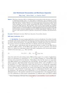
FIG. 1. 共Color online兲 Example multipath realization from the K-sparse model 共stem兲, and the deconvolution estimate produced by the joint MAP deconvolution/classifier 共solid兲 at 10 dB SNR. K

h关n兴 = 兺 ␣i␦ 关n − di兴, i=1

with K = 15 nonzero coefficients, delays di drawn uniformly on 关0,99兴, ␣i = ⫾ e−␤di with randomly chosen sign, and decay parameter ␤ = 0.0240 chosen to mimic real underwater acoustic channels. An example realization of a filter h drawn from this model is shown in Fig. 1. The diagonal covariance matrix ⌺h is estimated from 1000 samples of the impulse response.

identified the class label. The recovered filter is a reasonable reconstruction of the true filter, but generally underestimates the amplitude of the first coefficients, and does not reliably reconstruct the tail of h. The gross errors can be ascribed to the fact that the optimization problem in Eq. 共4兲 is not convex, and to the mismatch between the Laplacian prior and K-sparse model. Classification results in Fig. 2 show that the proposed joint QDA classifier dominates the matched filter classifier for both Laplacian multipath in 共a兲 and 共b兲, and for multipath generated by the K-sparse model in 共c兲 and 共d兲. The means for each class used for 共a兲 and 共c兲 共well-separated means兲 are orthogonal, so the matched filter performs well despite ignoring the multipath. However, for 共b兲 and 共d兲 the means are similar, and the matched filter performs poorly compared to joint QDA. The joint MAP classifier performs well at low SNR, but as predicted, performance degrades as SNR increases. For truly sparse multipath in 共c兲 and 共d兲, the joint MAP approach is unaffected for well-separated means in 共c兲, and affected moderately at high SNR for close means in 共d兲 compared to results using Laplacian multipath. Evidently, the ᐉ1 is an appropriate heuristic for the K-sparse multipath model; using ᐉ1 criteria to obtain sparse solutions is a popular approach.28

C. Signal-based joint QDA and joint MAP results

Figure 1 shows a reconstructed multipath estimate produced by the joint MAP deconvolution/classifier corresponding to the chosen class for the well-separated means experiment at 10 dB SNR. In this case, joint MAP correctly

IV. QDA CLASSIFICATION OF SIGNALS CORRUPTED BY LTI FILTERING USING FEATURES

Blind signal deconvolution and the proposed joint MAP and signal-based joint QDA methods are computationally

(a)

100

90 80 70 60 50

Joint QDA Matched Filter Joint MAP Blind Deconv + MF

−10 −8 −6 −4 −2 0 2 SNR (dB)

4

6

Correct classification (%)

Correct classification (%)

100

8 10 (b)

(c)

90 80 70 60 50 −10 −8 −6 −4 −2 0 2 SNR (dB)

80 70 60 50 −10 −8 −6 −4 −2 0 2 SNR (dB)

4

6

8 10

4

6

8 10

100 Correct classification (%)

Correct classification (%)

100

90

4

6

8 10 (d)

90 80 70 60 50 −10 −8 −6 −4 −2 0 2 SNR (dB)

FIG. 2. 共Color online兲 Classification accuracy for four experiments using multipath generated from a Laplacian model in 共a兲 and 共b兲, and a K-sparse model in 共c兲 and 共d兲. The results are averaged over 1000 i.i.d. test signals for each SNR point. J. Acoust. Soc. Am., Vol. 124, No. 5, November 2008

H. S. Anderson and M. R. Gupta: Joint deconvolution and classification

2977

prohibitive for signals captured at high sample rates. For M-length sampled signals, Cabrelli’s method requires the inversion of an M ⫻ M Toeplitz matrix, which at best is of complexity O共M log M兲. The joint MAP deconvolution requires more iterations to converge as M increases, and requires 共as does joint QDA兲 inversion of an M ⫻ M covariance matrix, which in general is complexity O共M 3兲. To decrease the computational burden and possibly increase classification performance, an alternative is to classify based on features that represent important characteristics of the signals and provide good class discrimination.29 The hope is that classes can be well-discriminated by features of significantly smaller dimensionality d Ⰶ M. Unless multipath-invariant features are used, a classifier trained on x-space features will not generally be applicable to classify the features of z共t兲 directly. However, if a functional relationship can be found that relates x-space features to their images in z-space, then a suitable classifier can be trained and applied in z-space. We show that such a relationship can be derived for subband power features, which represent an important class of discriminating features for many remotesensing applications. Extending the proposed joint QDA classifier to subband features in z-space requires expressing the mean and covariance of the subband power feature vector for z共t兲 in terms of statistics of the subband power features of the channel and training data. Let the d-dimensional feature vector Pz = 关Pz共f 1兲 ¯ Pz共f d兲兴T be composed of the subband powers of z共t兲 at frequencies 兵f i其 for i = 1 , . . . , d. Then for any frequency f, because Pz共f兲 = Z共f兲Z*共f兲, and Z共f兲 = X共f兲H共f兲 + W共f兲, the subband power can be expressed as Pz共f兲 = Px共f兲Ph共f兲 + Pw共f兲 + 2 Re兵X共f兲H共f兲W*共f兲其,

共9兲

where Px共f兲, Ph共f兲, and Pw共f兲 denote the power of the signal, the channel, and the noise for frequency f, respectively. Based on Eq. 共9兲, derivations for the mean and covariance of the feature vector Pz are given in the Appendix. For these derivations, it is assumed that w共t兲 is a realization of a Gaussian white noise process. The class-conditional mean feature vector ␮ Pz兩y can be expressed in terms of the noise power ␴w2 and mean vectors of the clean signal features and channel features, ␮ Px兩y and ␮ Ph, respectively, as

␮ Pz兩y = ␮ Px兩y · ␮ Ph + ␴w2 1,

共10兲

where · denotes Hadamard 共Schur or element-wise兲 multiplication, and 1 is a vector of ones. The class-conditional covariance ⌺ Pz兩y can be expressed in terms of ␴w2 and secondorder statistics of Px 兩 y and Ph as ⌺ Pz兩y = ⌺ Px兩y · ⌺ Ph + ␴w4 I + ⌺ Ph · ␮ Px兩y␮TP 兩y + ⌺ Px · ␮ Ph␮TP x

+

2␴w2

diag兵␮ Px兩y · ␮ Ph其.

h

共11兲

It is assumed that ␮ Ph, ⌺ Ph, and ␴w2 can be estimated from the channel. The statistics ␮ Px兩y and ⌺ Px兩y are estimated from training data for each class. Together, these statistics are used to compute class-conditional QDA model parameters ␮ Pz兩y and ⌺ Pz兩y from Eqs. 共10兲 and 共11兲 and, hence, build a QDA subband power feature classifier in the z-space. A. Informed and blind classifiers using features

To evaluate the proposed z-space joint QDA using power features, we consider two alternate approaches to classification from power features. First, an “informed” x-space classifier approach uses the expectation of the channel’s subband power response E关Ph兴 and the noise power ␴w2 to transform the z-space features to x-space by subtracting the noise power and deconvolving by E关Ph兴: Pˆx共f i兲 = 共Pz共f i兲 − ␴w2 兲 / E关Ph共f i兲兴. This approach uses the mean but not covariance of the channel. Second, a “blind” x-space classifier approach uses x-space features, and simply ignores statistics of the channel and noise altogether. Training signals are first normalized by their total power before a classifier is trained. Then, a received signal z共t兲 is also normalized by its total power before extracting features. We compare joint QDA to both blind and informed approaches for QDA, 1-NN, and a support vector machine 共SVM兲.25 B. Simulated classification experiments using joint QDA with power features

We consider the task of classifying narrow-band signals corrupted by unknown multipath due to propagation in a −3

x 10 1

amplitude

0.5 0 −0.5 −1

(a)

(b)

0

0.2

0.4 0.6 time (s)

0.8

1

FIG. 3. 共Color online兲 共a兲 Simulated ocean bathymetry with a single receiver 共marked by 䉺兲 at 共0 , 0 , −50兲 m, and 共b兲 a sample channel impulse response for a source located at 共460, 250, −70兲 m, generated by the Sonar Simulation Toolset 共Refs. 30 and 31兲. 2978

J. Acoust. Soc. Am., Vol. 124, No. 5, November 2008

H. S. Anderson and M. R. Gupta: Joint deconvolution and classification

TABLE II. Pole magnitude distribution for feature-based classification experiments. Parameter

Class 1

共

⌺a兩y

Class 2

兲

共

1.00 0.99 ⫻ 10−6 0.99 9.00

兲

6.00 −0.80 ⫻ 10−4 −0.80 1.00

Close poles

␮a兩y

共0.945 0.905兲

␮a兩y

Moderately-separated poles 共0.945 0.875兲 共0.879 0.948兲

␮a兩y

Well-separated poles 共0.965 0.875兲 共0.875 0.948兲

共0.909 0.948兲

shallow ocean channel. To simulate two classes of narrowband signals with two subband power features, training and test signals are generated i.i.d. using the z-domain model X兩y关z兴 =

共z − 1兲共z + 1兲 2 ⌸ᐉ=1 共z

* 兲 − pᐉ兩y兲共z − pᐉ兩y

共12兲

,

where the location of each class-conditional pole pᐉ兩y, ᐉ 苸 兵1,2其 is drawn randomly from the model aᐉ兩y exp共j␪ᐉ兲, where ␪ᐉ is fixed, and aᐉ兩y = 关a1兩y , a2兩y兴T is multivariate Gaussian distributed with mean ␮a兩y and covariance matrix ⌺a兩y. Although the vector a for each class is Gaussian distributed, the signals in feature space are not, as per Eq. 共12兲. Figure 4 shows an example pole-zero plot and corresponding logfeature space scatterplot for a well-separated case. We consider three instances of the experiment for choices of ␮a兩y that result in different class separation. The parameters ␮a兩y and ⌺a兩y for each instance of the experiment are shown in 1 Table II, and ␪1 = 50 and ␪2 = 51 . Note that since all poles and zeros lie within the unit circle, for each case the selected parameters correspond to a realization of a minimum phase signal, which could be produced from natural sources. Test and training signals were generated by taking i.i.d. draws of poles as described above, and taking 5000 evenly spaced samples around the unit circle of the complex z-plane, so that the length of each signal corresponds to

1.25 s, sampled at 4 kHz. At frequencies ␪1 and ␪2 the subband power is extracted from each signal and used as classification features. The parameters in Table II were chosen such that the generated test and training signals were linearly separable in the subband power feature space. Channel impulse responses h were drawn i.i.d. in the following manner. A receiver is placed at a depth of 50 m in a simulated shallow water channel, as shown in Fig. 3. Source locations were drawn uniformly from the cube 2 km across north and east and 150 m deep; locations falling below the ocean floor are discarded and redrawn. Channel impulse responses h were generated by propagating an impulsive source from the random source locations to the receiver using the CASS Eigenray routine provided in the Sonar Simulation Toolset.30 Impulse responses were sampled at 4 kHz. The ocean environment is set up to be fairly extreme, but static. We have imposed a prototypical sound speed profile 共ranging from 1477 to 1492 m / s兲, and have modeled the ocean bottom to contain sandy gravel with mean grain size 2 mm. Surface roughness is governed by the wind speed, which is set to 15 km/ h. The channel geometry and a sample channel impulse response are shown in Fig. 3. Maximum likelihood estimates of ␮ Px兩y and ⌺ Px兩y were computed from 1000 randomly drawn training signals, and maximum likelihood estimates of ␮ Ph and ⌺ Ph were computed from 1000 randomly drawn channel impulse responses. The test samples were corrupted with randomly drawn multipath, and then i.i.d. white noise with variance ␴w2 was added, where the multipath-corrupted-signal to noise ratio was varied between −10 and 10 dB. Classification results were averaged over 5000 trials for each SNR. We compare the proposed z-space joint QDA classifier to x-space QDA, SVM with a linear kernel, and 1-NN classifiers using both the informed and blind approaches described in Sec. IV A. In each of the three simulations, the training and test data were linearly separable. Therefore, we set the regularization term C in the linear SVM 共Ref. 32兲 to a large value, C = 107. Then, none of the classifiers requires cross-validation. 3

10

power at θ2

Imaginary Part

1 0.5 0 −0.5 1

−1

(a)

2

10

−1

−0.5

0 0.5 Real Part

1

10 1 10

(b)

2

10 power at θ1

3

10

FIG. 4. 共Color online兲 共a兲 Pole-zero plot showing the mean location of the poles for each class 1 共⫻兲 and class 2 共ⴱ兲 for the “well-separated” case, and 共b兲 scatter-plot of the classes in log-feature space. J. Acoust. Soc. Am., Vol. 124, No. 5, November 2008

H. S. Anderson and M. R. Gupta: Joint deconvolution and classification

2979

100

QDA in z−space QDA in x−space (informed) QDA in x−space (blind) SVM in x−space (informed) SVM in x−space (blind) 1−NN in x−space (informed) 1−NN in x−space (blind)

Correct classification (%)

90

80

70

60

50

(a)

−10

−8

−6

−4

−2

0 SNR (dB)

2

4

6

8

10

−8

−6

−4

−2

0 SNR (dB)

2

4

6

8

10

100

Correct classification (%)

90

80

70

60

50

(b)

−10

100

Correct classification (%)

90

80

70

E. Bowhead whale song results

60

50

(c)

year to year. Therefore, we hope to be able to acoustically discriminate between two individuals based on previously recorded vocalizations. Our experimental setup simulates a shallow ocean channel 共in comparison to the observation distances兲, and low SNR. Each of the signals has non-negligible interfering noise from bearded seals, sea ice and banging hydrophone cables.33 The vocalizations were recorded in April 1988 near the coast of Point Barrow, Alaska, but for these experiments, we inject the signals into randomly drawn locations in the simulated bathymetry shown in Fig. 3共a兲. Example vocalizations for each whale are shown in Fig. 6. Classifiers were trained on five training signals drawn at random for each class. The remaining 14 signals were propagated from a random source location in the bathymetry to the receiver using the CASS Eigenray routine. Gaussian white noise is added to the multipath signal to achieve a specified SNR. To increase the statistical significance of the results, classification results were averaged over 1000 iterations of the random training/test partitioning with random source locations. For classification, four peak power features were selected: the two largest amplitude peaks averaged over signals in class 1 共163 and 258 Hz兲 and the two largest amplitude peaks for class 2 共588 and 207 Hz兲. Features do not correspond to strong interfering noise, and result in classes that, prior to the channel effects, are 100% linearly separable. As before, we compare the z-space joint QDA classifier to x-space QDA, linear SVM, and 1-NN classifiers using both informed and blind approaches.

−10

−8

−6

−4

−2

0 SNR (dB)

2

4

6

8

10

FIG. 5. 共Color online兲 Results for feature-based classification on simulated data for the experiments where classes are 共top兲 close in feature space, 共middle兲 moderately separated in feature space, and 共bottom兲 well-separated in feature space.

Results for the Bowhead whale songs are shown in Fig. 7. The z-space joint QDA classifier using power features consistently achieves roughly 4% higher accuracy than other methods across the range of SNRs. This can be ascribed to the fact that the multipath channel distorts the relative covariance structures of class 1 and class 2 whale vocalizations. V. CONCLUSIONS AND OPEN QUESTIONS

C. Simulation results

Results for each experiment are shown in Fig. 5. The joint QDA method using features 共QDA in z-space兲 performs markedly better than the other approaches when the classes are difficult to separate. As class separation increases, the performance of the z-space QDA and informed SVM and 1-NN become similar. D. Classifying bowhead whale songs in multipath channel

We employ the feature-based joint QDA method to identify individual Bowhead whales in a multipath environment by classifying the end notes of their songs. Several end notes of Bowhead whale vocalizations for two individuals were extracted from the MobySound archive.33 Fifteen vocalizations are available for whale 1, and nine vocalizations are available for whale 2. According to the metadata, the end notes of Bowhead whale songs are relatively stable from 2980

J. Acoust. Soc. Am., Vol. 124, No. 5, November 2008

We have presented classification methods that jointly consider the effects of multipath distortion with classification. In particular, we have investigated a joint MAP deconvolution/classifier that incorporates first- and secondorder statistics of the channel and yields a MAP solution for the recovered signal xˆ, the recovered filter hˆ, and the class estimate y *. Two drawbacks of the joint MAP algorithm are that it is not convex, and that it theoretically performs poorly at high SNR. The first problem might be addressed by maximizing the marginal p共h , y 兩 z兲 which yields a convex expression, but requires more complicated optimization approaches. The second problem arises since regularization scales with the noise power ␴w2 , which may be replaced by a fixed penalty that can be chosen via cross-validation. We hypothesized that better classification performance can be gained by marginalizing over x and h. To that end, we presented a joint QDA classifier that accounts for the LTI corruption probabilistically. Experiments showed that the joint QDA classifier outperformed the joint MAP classifier H. S. Anderson and M. R. Gupta: Joint deconvolution and classification

1500

1500

Frequency (Hz)

2000

Frequency (Hz)

2000

1000

1000

500 0

500 0

0

(a)

1

2

Time (s)

3

0

(b)

1

Time (s)

2

3

FIG. 6. 共Color online兲 Spectrograms of whale song-endnotes for 共a兲 the first Bowhead whale and 共b兲 the second Bowhead whale. The vocalizations of the second whale tend to be more variable, cover a greater dynamic range, and contain stronger harmonic components than the first whale. Notice that the vocalization in 共a兲 contains interfering calls from a bearded seal from about 800 to 1200 Hz.

and a classifier based on blind deconvolution. Further, we derived a joint QDA classifier that classifies based on subband power features. Experiments on both simulated signals and real Bowhead whale vocalizations demonstrated the efficacy of the joint QDA classifier using features. Although we have derived the joint QDA classifier for subband power features, there are many other important classes of features for signal processing including real cepstrum, wavelets, and wavepacket decomposition.12 In cases where the features are linear functions of the data, such as the shift invariant wavepackets described in Ref. 12, the derivation of a joint QDA classifier is straightforward. However, features that are nonlinear functions of the received signal 共e.g., real cepstrum兲 may require low-order approximate solutions. We compared the joint QDA classifier on subband features to other classifiers that also took into account the mean multipath using subband power features. We showed that using this first-order multipath information significantly improved performance over ignoring the multipath altogether, except in the simulation experiment with well-separated classes and low noise. An open question in this line of research is how to take advantage of further information about the multipath for other classifiers, such as the nearestneighbor and support vector machine classifiers.

APPENDIX: DERIVATIONS

In the Appendix, we use x, h, w, and z 共and hence, all functions of them, for example Px兲 to denote random signals, not their realizations as done in the main body. Derivation of the first and second moments of z„t…

This section details the derivation of Eqs. 共7兲 and 共8兲. Since the noise is zero-mean, the nth component of the mean time signal ␮z兩y is

␮z兩y关n兴 = E关共x ⴱ h兲关n兴 + w关n兴兩y兴 = E

冋兺

x关k兴h关n − k兴兩y

k

册

= 兺 E关x关k兴兩y兴E关h关n − k兴兴 = 兺 ␮x兩y关k兴␮h关n − k兴, k

k

and thus ␮z兩y = ␮x兩y ⴱ ␮h. The covariance matrix is derived: ⌺z兩y = E关zzT兩y兴 − E关z兩y兴E关z兩y兴T 共a兲

T = E关共x ⴱ h兲共x ⴱ h兲T兩y兴 + E关wwT兴 − ␮z兩y␮z兩y

共b兲

T = E关共xxT兲 ⴱⴱ 共hhT兲兩y兴 + ␴w2 I − ␮z兩y␮z兩y

共c兲

T , = E关xxT兩y兴 ⴱⴱ E关hhT兴 + ␴w2 I − ␮z兩y␮z兩y

100

where the expectations are taken with respect to the appropriate distributions. In the above, 共b兲 follows from 共a兲 because the 共m , n兲th component of the outer product 共x ⴱ h兲 ⫻共x ⴱ h兲T can be expressed as

Correct classification (%)

90 80

冉兺

70 60

QDA in z−space QDA in x−space (informed) QDA in x−space (blind) SVM in x−space (informed) SVM in x−space (blind) 1−NN in x−space (informed) 1−NN in x−space (blind)

50 40 30 −10

−8

−6

−4

−2

0 SNR (dB)

2

4

6

8

冊冉兺 i

x关i兴h关m − i兴

冊

= 兺 兺 x关k兴h关n − k兴x关i兴h关m − i兴 k

10

FIG. 7. 共Color online兲 Classification results for identifying Bowhead whales by the end-notes of their songs. The SVM in x-space 共blind兲 and 1-NN in x-space 共blind兲 mostly overlap one another. Note that unlike previous figures, the ordinate axis shows results down to 30% correct classification to better show the trend over SNR. J. Acoust. Soc. Am., Vol. 124, No. 5, November 2008

x关k兴h关n − k兴

k

i

= 兺 兺 共x关k兴x关i兴兲共h关n − k兴h关m − i兴兲, k

i

and thus 共x ⴱ h兲共x ⴱ h兲T = 共xxT兲 ⴱⴱ共hhT兲. Then, 共c兲 follows from 共b兲 due to the linearity of both expectation and convolution. Finally, 共c兲 can be rewritten as Eq. 共8兲.

H. S. Anderson and M. R. Gupta: Joint deconvolution and classification

2981

Derivation of the first and second moments of Pz„f…

This section details the derivation of Eqs. 共10兲 and 共11兲. Let ␮ Pz兩y = E关Pz 兩 y兴, ␮ Px兩y = E关Px 兩 y兴, ␮ Ph = E关Ph兴 and E关Pw兴 = E关WW*兴 = ␴w2 1 by assumption, where 1 is a vector of ones. The first moment given by Eq. 共10兲 follows from Eq. 共9兲 since E关Re兵a其兴 = E关 21 共a + a*兲兴 = 21 共E关a兴 + E关a兴*兲 = Re兵E关a兴其, and X共f兲, H共f兲, and W*共f兲 are independent, so E关Re兵X共f兲H共f兲W*共f兲其兴 = 0 because E关W*共f兲兴 = 0. The fact that E关W*共f兲兴 = 0 follows from E关w共t兲兴 = 0 and the independence of the noise random process over time. For the class-conditional covariance ⌺ Pz兩y, we derive the second moment and cross-correlation separately. For notational simplicity, we denote E关x 兩 y兴 by E关x兴, that is, the classconditional membership is implied in the expectation. For the second moment, it follows from Eq. 共9兲 that 共a兲

E关Pz共f兲2兴 = E关P2x P2h + Pw2 + 4 Re共XHW*兲2 + 4共Px Ph + Pw兲Re共XHW*兲 + 2Px Ph Pw兴 共b兲

2E关Re共X jH jW j兲共Pxi Phi + Pwi兲兴 = E关共X jH jW j + X*j H*j W*j 兲 ⫻共XiXi*HiHi* + WiWi*兲兴. After multiplication, the above consists of four terms, each containing a single W j. Since W j is uncorrelated with every other random variable and E关W j兴 = 0, each of the four terms in the expansion has zero mean, and thus the entire expression is zero. By the same logic, the sixth term of of Eq. 共A2兲 is 2E关Re共XiHiWi兲共Px j Ph j + Pw j兲兴 = 0. The last term of Eq. 共A2兲 can be rewritten 4E关Re共XiHiWi兲Re共X jH jW j兲兴 = E关共XiHiWi + Xi*Hi*Wi*兲 ⫻共X jH jW j + X*j H*j W*j 兲兴. Taking the product results in four terms which each have a single Wi and W j. Since Wi and W j are uncorrelated and each has zero-mean, each of the four terms is zero. Thus, the cross-correlation of any two frequencies f i ⫽ f j is

= E关P2x 兴E关P2h兴 + E关Pw2 兴 + 4E关Re共XHW*兲2兴

E关Pzi Pz j兴 = E关Pxi Px j兴E关Phi Ph j兴 + E关Pxi兴E关Phi兴E关Pw j兴

+ 2E关Px兴E关Ph兴E关Pw兴 共c兲

= E关P2x 兴E关P2h兴

+

E关Pw2 兴

+ E关Px j兴E关Ph j兴E关Pwi兴 + E关Pwi兴E关Pw j兴. + 2E关XX*HH*WW*

+ Re共共XHW*兲 兲兴 + 2E关Px兴E关Ph兴E关Pw兴 2

Conditioning on the class label y, Eqs. 共A1兲 and 共A3兲 can be combined into a single covariance matrix, where the 共i , j兲th element is

共d兲

⌺ Pz兩y关i, j兴 = 共⌺ Px兩y关i, j兴 + ␮ Px兩y关i兴␮ Px兩y关j兴兲共⌺ Ph关i, j兴

= E关P2x 兴E关P2h兴 + E关Pw2 兴 + 4E关Px兴E关Ph兴E关Pw兴

+ ␮ Ph关i兴␮ Ph关j兴兲 + 共⌺ Pw关i, j兴 + ␮ Pw关i兴␮ Pw关j兴兲

+ 2 Re共E关XX兴E关HH兴E关W*W*兴兲

+ 共␮ Px兩y关i兴␮ Ph关i兴␮ Pw关j兴

共e兲

= E关P2x 兴E关P2h兴 + E关Pw2 兴 + 4E关Px兴E关Ph兴E关Pw兴. 共A1兲

In the above, 共b兲 follows from 共a兲 because 4E关共Px Ph + Pw兲Re共XHW*兲兴 can be expanded into the sum of two terms containing E关W*兴 and E关W*WW*兴, and since these terms equal zero, 4E关共Px Ph + Pw兲Re共XHW*兲兴 = 0. For 共c兲, we employed the identity 共Re兵c其兲2 = 1 / 2共cc* + Re共c2兲兲. Then 共d兲 follows from 共c兲 by the definition of power and the interchangeability of expectation and the real operator, explained earlier in this section. The step from 共d兲 to 共e兲 holds because the Fourier transform W共f兲 = F关w共t兲兴 of a zero-mean Gaussian white noise process is a complex zero-mean Gaussian white process with Re共W兲 and Im共W兲 uncorrelated, E关Re共W兲兴 = E关Im共W兲兴 = 0, and E关Re共W兲2兴 = E关Im共W兲2兴= 21 ␴w2 , so that E关W*W*兴 = E关Re共W兲2 − 2j Re共W兲Im共W兲 − Im共W兲2兴 = 0.34 Last, we derive the cross-correlation using as short-hand Pzi to denote Pz共f i兲, Phi to denote Ph共f i兲, Hi to denote H共f i兲, etc. From Eq. 共9兲, for i ⫽ j, E关Pzi Pz j兴 = E关Pxi Phi Px j Ph j兴 + E关Pxi Phi Pw j兴 + E关Px j Ph j Pwi兴 + E关Pwi Pw j兴 + 2E关Re共X jH jW j兲 ⫻共Pxi Phi + Pwi兲兴 + 2E关Re共XiHiWi兲共Px j Ph j + Pw j兲兴 + 4E关Re共XiHiWi兲Re共X jH jW j兲兴, 共A2兲 Consider the fifth term of Eq. 共A2兲, 2982

J. Acoust. Soc. Am., Vol. 124, No. 5, November 2008

共A3兲

+ ␮ Px兩y关j兴␮ Ph关j兴␮ Pw关i兴兲共1 + ␦ij兲 − ␮ Pz兩y关i兴␮ Pz兩y关j兴 = ⌺ Px兩y关i, j兴⌺ Ph关i, j兴 + ⌺ Pw关i, j兴 + ␮ Px兩y关i兴␮ Px兩y关j兴⌺ Ph关i, j兴 + ⌺ Px兩y关i, j兴␮ Ph关i兴␮ Ph关j兴 + 2␮ Px兩y关i兴␮ Ph关i兴␮ Pw关i兴␦ij = ⌺ Px兩y关i, j兴⌺ Ph关i, j兴 + ␴w4 ␦ij + ␮ Px兩y关i兴␮ Px兩y关j兴⌺ Ph关i, j兴 + ⌺ Px兩y关i, j兴␮ Ph关i兴␮ Ph关j兴 + 2␴w2 ␮ Px兩y关i兴␮ Ph关i兴␦ij , where ␦ij = 1 if i = j or 0 otherwise. The last step in the derivation holds since E关Pw共f i兲Pw共f j兲兴 = E关WiWi*W jW*j 兴 is 2共␴w2 兲2 for i = j or is 共␴w2 兲2 for i ⫽ j by Isserlis’ Gaussian moment theorem,35 and ␮ Pw关i兴 = ␴w2 . The result is rewritten in compact form in Eq. 共11兲. 1

R. L. Field, “Transient signal distortion in a multipath environment,” Proc. OCEANS 1990, pp. 111–114. 2 D. W. Tufts, I. Kirsteins, R. J. Vaccaro, C. S. Ramalingam, and A. Shah, “Improvements in signal processing for time-varying multipath propagaH. S. Anderson and M. R. Gupta: Joint deconvolution and classification

tion environments,” Proc. OCEANS, 1991, Vol. 1, pp. 586–593. S. Senmoto and D. Childers, “Signal resolution via digital inverse filtering,” IEEE Trans. Aerosp. Electron. Syst. 8, 644–640 共1972兲. 4 J. E. Ehrenberg, T. E. Ewart, and R. D. Morris, “Signal-processing techniques for resolving individual pulses in a multipath signal,” J. Acoust. Soc. Am. 63, 1861–1865 共1978兲. 5 T. E. Ewart, J. E. Ehrenberg, and S. A. Reynolds, “Observations of the phase and amplitude of individual Fermat paths in a multipath environment,” J. Acoust. Soc. Am. 63, 1801–1808 共1978兲. 6 F. B. Shin, D. H. Kil, and R. Wayland, “IER clutter reduction in shallow water,” Proc. IEEE ICASSP, 1996, pp. 3149–3152. 7 D. J. Strausberger, E. D. Garber, N. F. Chamberlain, and E. K. Walton, “Modeling and performance of HF/OTH radar target classification systems,” IEEE Trans. Aerosp. Electron. Syst. 28, 396–403 共1992兲. 8 G. Okopal and P. Loughlin, “Feature extraction for classification of signals propagating in channels with dispersion and dissipation,” Proc. SPIE 6566, April 9–13, 2007. 9 H. Liu, P. Runkle, and L. Carin, “Classification of distant targets situated near channel bottoms,” J. Acoust. Soc. Am. 115, 1185–1197 共2004兲. 10 D. A. Caughey and R. L. Kirlin, “Blind deconvolution of echosounder envelopes,” Proc. IEEE ICASSP, 1996, pp. 3149–3152. 11 M. J. Roan, M. R. Gramann, J. G. Erling, and L. H. Sibuld, “Blind deconvolution applied to acoustical systems identification with supporting experimental results,” J. Acoust. Soc. Am. 114, 1988–1996 共2003兲. 12 D. H. Kil and F. B. Shin, Pattern Recognition and Prediction with Applications to Signal Characterization 共American Institute of Physics Press, Woodbury, NY, 1996兲. 13 M. K. Broadhead and L. A. Pflug, “Performance of some sparseness criterion blind deconvolution methods in the presence of noise,” J. Acoust. Soc. Am. 107, 885–893 共2000兲. 14 Q. Zhu and B. Steinberg, “Correction of multipath interference using clean and spatial location diversity,” Proc. IEEE Ultrasonics Symp., 1995, pp. 1367–1370. 15 R. A. Wiggins, “Minimum entropy deconvolution,” Geoexploration 16, 21–35 共1978兲. 16 C. A. Cabrelli, “Minimum entropy deconvolution and simplicity: A noniterative algorithm,” Geophysics 50, 394–413 共1984兲. 17 M. R. Gupta, H. S. Anderson, and Y. Chen, “Joint deconvolution and classification for signals with multipath,” Proc. IEEE ICASSP, 2007. 18 M. R. Gupta and H. Anderson, “Maximum likelihood signal classification using second-order blind deconvolution probability model,” Proc. IEEE Wkshp. Stat. Sig. Proc., 2007. 3

J. Acoust. Soc. Am., Vol. 124, No. 5, November 2008

19

N. Dasgupta and L. Carin, “Time-reversal imaging for classification of submerged elastic targets via Gibbs sampling and the relevance vector machine,” J. Acoust. Soc. Am. 117, 1999–2011 共2005兲. 20 A. K. Jain, Fundamentals of Digital Image Processing 共Prentice Hall, Englewood Cliffs, NJ, 1989兲. 21 A. Kirsch, An Introduction to the Mathematical Theory of Inverse Problems 共Springer, New York, 1996兲. 22 S. Boyd and L. Vandenberghe, Convex Optimization 共Cambridge University Press, Cambridge, 2004兲. 23 R. W. Yeung, A First Course in Information Theory 共Springer, New York, 2002兲. 24 E. Y. Lam and J. W. Goodman, “Iterative statistical approach to blind image deconvolution,” J. Opt. Soc. Am. A 17, 1177–1184 共2000兲. 25 T. Hastie, R. Tibshirani, and J. Friedman, The Elements of Statistical Learning 共Springer, New York, 2001兲. 26 J. H. Friedman, “Regularized discriminant analysis,” J. Am. Stat. Assoc. 84, 165–175 共1989兲. 27 S. Srivastava, M. R. Gupta, and B. A. Frigyik, “Bayesian quadratic discriminant analysis,” J. Mach. Learn. Res. 8, 1287–1314 共2007兲. 28 E. Candes, “Compressive sampling,” Proc. Int. Congress of Math., 2006, Vol. 3, pp. 1433–1452. 29 R. O. Duda, P. E. Hart, and D. G. Stork, Pattern Classification, 2nd ed. 共Wiley, New York, 2001兲. 30 R. P. Goddard, “The Sonar Simulation Toolset,” Proc. OCEANS, 1989, Vol. 4, pp. 1217–1222. 31 R. P. Goddard, “The Sonar Simulation Toolset, Release 4.1: Science, mathematics and algorithms,” Technical Report APL-UW TR 0404, Applied Phyics Laboratory, University of Washington, 2005; URL http:// stinet.dtic.mil/cgi-bin/GetTRDoc?AD⫽ADA430617&Location⫽U2&doc ⫽GetTRDoc.pdf 共Last viewed August 2008兲. 32 R. E. Fan, P. H. Chen, and C. J. Lin, “Working set selection using the second order information for training SVM,” J. Mach. Learn. Res. 6, 1889–1918 共2005兲. 33 D. K. Mellinger and C. W. Clark, “Mobysound: A reference archive for studying automatic recognition of marine mammal sounds,” Appl. Acoust. 67, 1226–1242 共2006兲; http://hmsc.oregonstate.edu./projects/MobySound/ 共Last viewed: August 2008兲. 34 C. Therrien, Discrete Random Signals and Statistical Signal Processing 共Prentice Hall, Upper Saddle River, NJ, 1992兲. 35 L. Isserlis, “On a formula for the product-mean coefficient of any order of a normal frequency distribution in any number of variables,” Biometrika 12, 134–139 共1918兲.

H. S. Anderson and M. R. Gupta: Joint deconvolution and classification

2983