KOHONEN SELF-ORGANIZING FEATURE MAP IN PATTERN RECOGNITION
Markus Törmä Institute of Photogrammetry and Remote Sensing Helsinki University of Technology
[email protected]
Traditional statistical pattern recognition models have been studied quite a long time. Due to the difficulty of pattern recognition task (for example classification) there are many different models for that task. The need for a general model which could be successful in most pattern recognition tasks has led to study new approaches like neural networks and fuzzy sets. This paper introduces one self-organizing neural network, the Kohonen self-organizing feature map, and represents its use in different pattern recognition tasks.
1. INTRODUCTION The pattern recognition process for satellite image goes as follows. First, the instrument in the satellite makes its measurements and transfers the data to ground. Then in the preprocessing stage, the errors introduced by the measurement situation are corrected. These errors include geometrical errors due to the round earth and satellite movement and radiometrical errors due to the atmosphere and instrument. At this stage, the measurements should be as error-free as possible. Then a feature selection and extraction is performed. The information content of measurements is enormous. There is usually a need to compress the information and to use only the information which is needed to perform our task. In feature selection, only necessary measurements are chosen for further processing. In feature extraction, original measurements are compressed using a transformation. The recognition stage can be divided to supervised and unsupervised classification. If we have known classes, we use the supervised classification. The recognition is more difficult if we do not know the classes and use an unsupervised classification. This paper discusses about the applicability of the Kohonen self-organizing feature map to these different parts of the pattern recognition process. Second chapter introduces the key ideas behind neural networks and third chapter the Kohonen selforganizing feature map. Fourth chapter discusses about the feature extraction in the spatial and spectral domains. Fifth and sixth chapters are about unsupervised and supervised classification. More detailed discussion about the Kohonen self-organizing feature map and its applications can be found in (Kohonen, 1995).
2. NEURAL NETWORKS There are two different approaches when the artificial neural networks are used. In the first approach, the artificial neural networks are modeled after true biological neural networks. The aim is to get as good approximation of a biological neural network as possible. The second approach concentrates on applying the principles of biological neural networks to some specific applications. In these applications the parallel and adaptive properties of biological neural networks are simulated. In other words, artificial neural networks try to imitate a biological nervous system and its properties like memory and learning (Kangas, 1994). It is necessary to specify the meaning of an artificial neural network. The following definition fits well to most neural network models (Kohonen, 1988): "Artificial neural networks" are massively parallel interconnected networks of simple (usually adaptive) elements and their hierarchical organizations which are intended to interact with the objects of the real world in the same way as biological nervous system do. So, an artificial neural network (referred as neural network after this) is a parallel, distributed signal or information processing system, consisting of simple processing elements, also called nodes. The processing elements can possess a local memory and carry out localized information processing operations. In the simplest case processing element sums weighted inputs and passes the result through nonlinear transfer function. The processing elements are connected via unidirectional signal channels called connections. The connections are usually weighted and those weights are adapted during training of the network. The learning of the network is based on the adaptation of the weights. The neural network models can be characterized using their properties like connection topologies, processing element capabilities, learning algorithms, problem solving capabilities etc., and models can differ greatly (Kohonen, 1990).
3. KOHONEN SELF-ORGANIZING FEATURE MAP (SOM) Kohonen Self-Organizing feature Map (SOM) is a neural network which modifies itself in response to input patterns. This property is called self-organization and it is achieved using competitive learning. The basic competitive learning means that a competition process takes place before each cycle of learning. In the competition process a winning processing element is chosen by some criteria. Usually this criteria is to minimize an Euclidean distance between the input vector and the weight vector. After the winning processing element is chosen, its weight vector is adapted according to the learning law used. SOM differs from the basic competitive learning so that instead of adapting only the winning processing element also the neighbours of the winning processing element are adapted. The self-organization property of SOM is based on the use of the neighbourhood of the winning processing element (Hecht-Nielsen, 1990).
SOM is the most widely used selforganizing neural network. Other similar kind of neural networks are based on adaptive resonance theory (ART (Carpenter, 1995), SONNET (Nigrin, 1993)), basic competitive learning (Intrator, 1995) or are modified from SOM (SCONN (Choi et.al., 1994)). SOM creates topologically ordered mappings between input data and processing elements of the map. Topological order means that if two inputs are similar, then the most active processing elements responding to the inputs are located near each other in the map and the weight vectors of the processing elements are arranged to an ascending or descending order, wi < wi+1 ∀ i or wi > wi+1 ∀ i (this definition is valid for 1-dimensional SOM). The motivation behind SOM is that some sensory processing areas of brain are ordered in similar way (Kangas 1994).
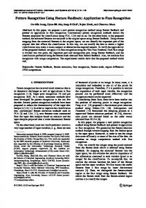
Processing elements
Weighted connections x1
x 2 ... x n Inputs
Figure 1: Two dimensional selforganizing feature map. Every input element has been connected to every output processing element via weighted connection.
SOM is usually represented as a two dimensional sheet (also other dimensions can be used) of processing elements (figure 1). Each processing element has its own weight vector, and the learning of SOM is based on the adaptation of these weight vectors (Kohonen, 1990). The basic idea is that the weight vectors of the processing elements approximate the probability density function of the input vectors. In other words, there are many weight vectors close to each other in the high density areas of the density function and less weight vectors in the low density areas. Figure 2 represents the distribution of image pixels taken from a Spot multispectral image, figure 2a is a sideview and figure 2b a topview. Figure 3 represents the placement of the weight vectors of 1dimensional SOM (81 processing elements). Figure 3a is a sideview and figure 3b a topview. The stars represent weight vectors and the lines connect nearest weight vectors. Figure 4 represents the placement of weight vectors of 2-dimensional SOM (9*9 processing elements). Figure 4a is a sideview and figure 4b a topview. Clearly, there are more weight vectors in the high density areas and less weight vectors in the low density areas. Mathematically speaking, SOM learns a continuous topological mapping f: B ⊂ n → C ⊂ m. This is nonlinear mapping from a n-dimensional space of input vectors to a m-dimensional space of SOM. Strict mathematical analysis exists only in simplified cases of SOM. It has been proved difficult to express the dynamic properties of SOM in mathematical theorems (Kohonen, 1990).
3.1 Basic SOM learning algorithm This version of SOM learning algorithm is based on (Lippmann, 1987): 1. 2. 3. 4.
5.
6.
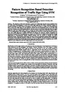
Initialize weights to small random values. Choose input randomly from the dataset. Compute Euclidean distance to all processing elements. Select the winning processing element ("best matching unit") c with the minimum distance. Update weight vectors of the winning processing element and its neighbourhood (figure 5) using the following learning law. The learning law moves the weight vector toward the input vector (figure 6).
NE c (t 1) NE c (t 2) c NE c (t 3)
Figure 5: One way to define the neighbourhood. The size of the neighbourhood is large in the beginning (NEc(t1)) and it decreases in time (NEc(t2) and NEc(t3)).
The gain term α should be near unity at the beginning of the training and decrease during training. The accurate rule for decreasing α is not important, it can be some linear or nonlinear function of time. First, the size of the neighbourhood NEc(t1) is large making rough ordering of SOM possible and the size is decreased (NEc(t2) and NEc(t3) as time goes on (figure 5). Finally, in the end only the winning processing element is adapted making the fine tuning of SOM possible. The use of neighbourhood makes topological ordering process possible and together with competitive learning makes the process nonlinear (Kohonen, 1990). Go to step 2 or stop the iteration when enough inputs are presented.
4. FEATURE EXTRACTION The information content of a typical multispectral satellite image is enormous. There is usually a need to compress information and use only that information which is needed to perform our pattern recognition task. The purpose of feature extraction is to transform the original satellite image so that the transformed image or images contain all the necessary information and redundant and useless information is lost. If we have one image (e.g. Spot Panchromatic), we perform the feature extraction in the spatial domain. This means that we seek important features from the image (e.g. edges or model texture) and form a new image which represents these features. If we have a multispectral image (e.g. Landsat TM), we perform the feature extraction in
spectral domain. This means that we decrease the dimensionality of the satellite image and maintain the information content of the image.
wi(t)
4.1 Feature extraction in spatial domain using SOM SOM can be used in feature extraction following way: take small windows from the image, transform windows to vectors, train SOM and check the weight vectors (transform them to images) if they correspond meaningful features.
x i(t) - w i(t)
wi(t+1) x i(t)
Figure 6: The learning law moves the weight vector toward the input vector. As a result, the weight vectors learn the density function of the input vectors.
Figure 7 represents weight vectors trained using 5*5 windows taken from inverted NDVI-image (figure 8). The size of SOM was 7*5 processing elements. NDVI-image was computed from SPOT XS channels 2 and 3. Darker areas correspond vegetated areas and lighter areas nonvegetated. Weight vectors have a clear order and they correspond to different targets found from the image. In other words, weight vectors have preformed a feature extraction. Weight vector (1,1) (upper left corner) is completely black corresponding to large vegetated areas and weight vector (7,5) is white corresponding large non-vegetated areas. Other weight vectors correspond to transitions to vegetated area to non-vegetated area and vice versa. Second plot in figure 8 represents large vegetated areas, whose closest weight vectors have been (1,1) and (2,2) (see also figure 7). Third plot in figure 10 represents large nonvegetated areas, whose closest weight vectors have been (7,4) and (7,5). Last plot in figure 10 represents some sharp transitions in vegetation, corresponding weight vectors (1,4), (3,5), (4,3) and (5,1). 4.2 Feature extraction in spectral domain using SOM SOM is usually arranged as a two dimensional matrix (also other dimensions can be used) of processing elements. As a result of learning phase, those processing elements which are spatially close to each other respond in a similar way to the presented input pattern. In other words, the map is topologically ordered. Also, SOM makes nonlinear transformation from a d-dimensional input space to a m-dimensional map space. The map space is defined by the coordinates of the processing elements. All these properties are useful in feature extraction. In feature extraction, the original feature vector is presented to SOM, and its winning processing element and its mapcoordinates are searched. These mapcoordinates could be used as a transformed features, but usually there is a limited number of processing elements and many different input vectors get same coordinates. This means that if the density function of input vectors is continuous, the density function of transformed vectors is not continuous.
A better way to make the transformation is to use distances computed during the search of the winning processing element. There are two alternatives: A.
B.
A weighted mean of mapcoordinates are computed using inverse distances from an input vector to weight vectors as weights. These mean values are used as a transformed vector. The coordinates of BMU are searched and distances computed from an input vector to BMU (dA) and the second closest weight vectors (dB) in row and column direction. The transformed value is coordinate of BMU ± dA / ( dA+dB ). The plus-sign is used, if the coordinate of the second closest weight vector is greater than the coordinate of BMU.
4.2.1 Experiments SOM was compared to a special case of Karhunen-Löwe transformation called principal component analysis (PCA). Datasets used were artificially created datasets (three different), data taken from a Landsat TM-image and data taken from several ERS-1 SAR-images. First feature extraction was made using SOM and PCA to dimension 2. Then the transformed features were classified using the Bayes rule for minimum error. The density function estimation was made using k-nearest neighbour method. The classification error was estimated using resubstitution and leave-one-out estimation methods. The criterion to compare results was minimize the classification error. Three different artificial datasets were used. The original dimension of dataset was 8 and number of classes 2. The datasets were generated using a random number generator. The number of samples per class was equal to the dimension times N, where N = 5, 10 or 100. Then generated samples were classified and the classification errors were estimated. This was repeated 50 times and each time the samples were generated independently. Finally, the statistical descriptors, mean value, median value, standard deviation, minimum and maximum values were computed from the classification errors. First dataset (II) had equal covariance matrices (identity matrices) and the mean vectors were different. Bayes error was about 10%. Second dataset (I4I) had equal mean vectors and the covariance matrix for first class was identity matrix I and for second class four times I. Bayes error was about 9%. Third dataset (IA) had different mean vectors and covariance matrices. Bayes error was about 1.9% (Fukunaga, 1990). The first real dataset was taken from a Landsat TM-image. The number of channels was six (TM channel 6 was not included). Data for six classes was determined using a digital land-use map and visual inspection. Classes were open land (3.9%), open rock (4.3%), forest (29.6%), swamp (11.6%), agricultural field (42.8%) and water (7.8%). The size of the dataset was 2390 vectors. The second real dataset consisted 14 ERS-1 SAR-images, taken at different times between June 1993 and March 1994. Data for five classes was determined using a digital land-use map and visual inspection. Classes were forest (20%), agricultural field (20%), urban area (20%), swamp (20%) and water (20%). The size of the dataset was 2500 vectors.
When artificial datasets were used, the classification errors using different feature extraction methods were quite the same, differences were small. The classification errors for dataset II varied between 28-34% for PCA and 32-39% for SOM. The classification errors for dataset I4I varied between 43-45% for PCA and 43-47% for SOM. The classification errors for dataset was about 10% for PCA and varied between 10-15% for SOM. The main difference occurred when the number of samples per class was small, then the classification errors with features computed using PCA were smaller than the classification errors with features computed using SOM. Another difference occurred when the dataset II was used, then the classification errors with features computed using PCA were also smaller. When the number of samples per class increased, the difference decreased. Real datasets were also classified before feature extraction. The classification error for Landsat dataset was about 16% and for ERS-1 dataset about 12%. When feature extraction was carried out using PCA, the classification error for Landsat dataset was about 18% and for ERS-1 dataset about 20%. When feature extraction was carried out using SOM, the classification error for Landsat dataset was about 16% and for ERS-1 dataset about 16%. In other words, using real datasets, SOM performs feature extraction better than PCA. Another advantage of SOM is that if the datasets are large, computing times are shorter.
5. CLUSTERING Clustering, also called unsupervised classification, is used to identify natural groupings of data. In clustering the classes of the available patterns are unknown and sometimes even the number of these classes is unknown. In this kind of problems, one attempts to find classes of patterns using some measure of similarity. Usually similarity is defined as proximity of the points in the measurement space according to a distance function, but similarity can be based on other properties such as the direction of the vectors in the measurement space (Jain, 1988). 5.1 1-dimensional SOM When 1-dimensional SOM is used in clustering, the simplest method is that the weight vectors of the processing elements correspond to the cluster mean vectors just like e.g. in k-means clustering algorithm. After the learning process, inputs are represented and each input is assigned to the nearest weight vector corresponding to an individual cluster. The advantages are that the method is fast and convergence to a suitable solution is certain. The drawback is that the number of clusters should be known in advance. Compared to the hard k-means clustering algorithm, 1-dimensional SOM converges faster, the quantization error is smaller and when repeated, the convergence to the same solution is more likely (Törmä, 1993).
b.
100
0 0
200 Wetness
100
c.
200
200 Wetness
Greenness
a.
100
0 0 100 200 0 100 200 0 Brightness Brightness Figure 9: The positions of the weight vectors, size of map 9*7.
100 200 Greenness
5.2 2-dimensional SOM The clustering using 2-dimensional SOM can be made using two different strategies. First, we can transform the input space to a map space and form clusters there. Secondly, we can form clusters in the weight space by agglomerating the weight vectors. Figure 9 represents the positions of the weight vectors (7x9 SOM) according to different coordinate axes. The explanation for the data can be found from chapter 4.3. 5.2.1 Method A - clustering in the map space When clustering is made in the map space, every processing element has been computed numerical value approximating the probability density function of the input vectors. This numerical value can be computed in several ways: 1.
2.
3. 4.
Count how many times each processing element is the winning processing element when whole inputdata is presented to SOM. The value in high density areas is big and vice versa. A drawback is that this method does not pay attention to the position of the weight vectors. Approximate the space reserved for each processing element by computing the average distance to the nearest weight vectors. The approximation of the probability density function is the inverse of this distance. A drawback is that this method does not pay attention to the number of the best matching units. Combine earlier methods. This method is similar to histogram density function estimation method (Devivjer, 1982). Compute the inverse mean quantization error for each processing element. The quantization error is the squared Euclidean distance between input vector and its winning processing element. For every processing element, the quantization errors are summed and divided by the number of corresponding input vectors. The inverse of the mean quantization error is computed so that the estimate of the density function would have big value in high density areas and vice versa. A drawback is that this method does not take care of the noncontinuity of the probability density function.
a.
b.
c.
d.
100
100
100
100
50
50
50
50
0
0
0
0
8
2 4 6
8
2
6
4
4
6
2
8
2
6
4
4
6
2
8
2
6
6
4
4
6
2
2
2
2
2
4
4
4
4
6
6
6
6
4 2
2 4 6 8 2 4 6 8 2 4 6 8 2 4 6 8 Figure 10: Wire-frame plots of the probability density function approximated by methods A1 - A4. Also clustered maps are shown.
After computing the approximation of the probability density function the clusters are determined using a simple gradient procedure. We take one processing element and search successor to it. The successor is found by computing the local gradient, meaning the maximum difference between neighbour processing elements. When the successor is found, it is linked to the processing element. This is repeated, unless we cannot find the successor for the processing element, or an already labelled processing element is found. If we cannot find a successor we have found the peak of the probability density function. This procedure is repeated unless all processing elements belong to some cluster. Figure 10a represents a wire-frame plot about the approximated probability density function (method A1) and clustered map (seven clusters). Figure 10b represents wireframe plot about the approximated probability density function (method A2) and clustered map (seven clusters). Figure 10c represents wire-frame plot about the approximated probability density function (method A3) and clustered map (six clusters). Figure 10d represents wire-frame plot about the approximated probability density function (method A4) and clustered map (five clusters). Methods A1 - A3 form quite similar kind of clustered maps and method A4 forms a different kind of clustered map.
b.
c.
200
100
200 Wetness
200 Wetness
Greenness
a.
100
100
0 0
0 0 100 200 0 100 200 0 100 200 Brightness Brightness Greenness Figure 11: Agglomeration of the weight vectors, intermediate state.
5.2.2 Method B - clustering in the weight space Another version assumes that SOM makes a good vector quantization, in other words, SOM moves the weight vectors of the processing elements to optimal places according to the density function of the input data. In this case, in high density areas there are many weight vectors and in low density areas less weight vectors. So, a natural way to form clusters is to move the weight vectors toward the direction of the gradient of the density function. The direction of the gradient of the density function, where weight vectors are moved, is estimated by computing the local mean of the neighbourhood of the weight vector (Fukunaga, 1990). This local mean is computed simply by searching k nearest weight vectors and computing their mean vector. The original weight vector is then replaced by the computed local mean. This process is repeated until weight vectors do not move. In the end, weight vectors are in clearly separable groups and weight vectors in one group correspond to one cluster. b.
0 0
100
200 Wetness
100
c.
200
200 Wetness
Greenness
a.
100
0 0 100 200 0 100 200 0 Brightness Brightness Figure 12: Agglomeration of the weight vectors, final state.
100 200 Greenness
Figure 11 represents the agglomeration of the weight vectors (compare this figure to figure 9). The weight vectors have been moved close to each other. a. Figure 12 represents the final state of 1 1 agglomeration. The weight vectors have 2 been moved to six clearly separable 2 3 3 groups. The value of nearest neighbours 4 used to compute the local mean was six. 4 5 5 Also figure 13 represents the clustered 6 6 maps, figure 13a represents the 7 intermediate result corresponding to the 7 2 4 6 8 2 weight vectors in figure 11 (24 clusters) and figure 13b represents the final result corresponding to the weight vectors in figure 12 (six clusters), which is closer to the method A4 than the Figure 13: Clustered maps. methods A1 - A3.
b.
4
6
8
5.3 Experiments In order to evaluate the presented clustering methods, a Landsat Thematic Mapper satellite image was clustered and compared to a digital land use map. The study area consists of ten different land use classes, but two classes, forest (56%) and agricultural field (29%) were dominant. In order to decrease the dimension of the feature space for easier visualization of data and speed computations, a Tasselled Cap transformation was performed. This transformation is a linear transformation and it rotates the coordinate axis so that the new coordinate axis are related to physical parameters. The coefficients of the transformation are determined empirically. The first transformed feature, called brightness, correspond to the soil reflectance. The second feature, greenness, correspond to the amount of green vegetation. The third feature, wetness, correspond to the soil and canopy moisture (Crist, 1984). Figure 14 represents the distribution of the transformed data. Examples in chapter 5.2 were made using a subset of the data, 10% about original was used.
Figure 14: Distribution of transformed data.
Experiments were made as follows: first the image was clustered using some of the presented methods, then the result was compared to a digital map. The comparison was made so that we chose cluster for the land use class according to which cluster represents that land use class best. The pixels belonging to other clusters were considered as erroneous pixels. Finally, the percentage of correctly classified pixels (classification accuracy) was computed. It was noted, that one cluster can represent several different land use classes and usually the classification accuracy decreased as number of clusters increased. When the number of clusters was four, the classification accuracy of 1-dimensional SOM was 46.7%. The best classification accuracy of 2-dimensional SOM with method A2 was 57.5% (size of SOM 9x7) and method B was 60.2% (size of SOM 11x9, number of neighbours 17). The problem with method B was that the accuracies varied much (44.9% - 60.2%) when the size of SOM and the number of neighbours were changed. So there is a need for a good method to evaluate the goodness of clustering result without the ground truth. When the number of clusters was seven, the classification accuracy of 1-dimensional SOM was 34.2%. The best classification accuracy for 2-dimensional SOM with method A4 was 48.6% (size of SOM 7x7) and method B was 41.3% (size of SOM 5x5, number of neighbours 1). Also in this case the problem with 2-dimensional methods were that the accuracies varied greatly (28.5% - 48.6%) when the size of SOM and number of neighbours were changed.
6. CLASSIFICATION SOM can also be used to classification applications. In this case, SOM is first trained in the usual way. After the training is complete, each processing element is labelled using the labelled data. Another way is to incorporate the information about correct class to learning. That means that the classnumber is included to input vector (Kohonen, 1995). If classification accuracy of SOM is not sufficient, the weight vectors can be finetuned using Learning Vector Quantization (LVQ) methods. These methods move codebook-vectors (=weight vectors) to optimal places using supervised learning. The simplest method, LVQ1, works as follows: codebook-vector closest to input vector is updated using the equation wc(t 1)
wc(t)
α(t) ( x(t)
wc(t) ),
wc(t)
α(t) ( x(t)
wc(t) ),
if x and wc belong to same class, wc(t 1)
if x and wc belong to a different class. Learning rate α(t) decreases in time and its initial value should be relatively small. The idea is to move the codebook-vector toward input vector if their classes match, otherwise the codebook-vector is moved further away (Kohonen, 1995). 6.1 Experiments The classification was carried out using SOM, LVQ1 and the Bayes rule for minimum error with k-nearest neighbour density function estimation method. The classification error was determined using resubstitution and holdout estimation methods. The dataset consisted 14 ERS-1 SAR-images, taken at different times between June 1993 and March 1994. The data for five classes was determined using a digital landuse map and visual inspection. The classes were forest (49.7%), agricultural field (5.9%), urban area (9.0%), swamp (12.3%) and water (23.1%). The data was divided to a trainingset (7940 vectors) and a testset (7940 vectors). When the dataset was classified using SOM, the resubstitution error estimate was 14.6% and the holdout estimate 14.7%. In LVQ1 classification, the resubstitution error estimate was 11.2% and the holdout estimate 11.2%. The best result was classification using the Bayes rule with k-nearest neighbour density estimation method, the resubstitution error estimate was 9.0% and the holdout estimate 10.1%. Advantage of SOM+LVQ1 is the computing speed. SOM+LVQ1 classification took little over one hour in IBM RS/6000 computer, when the classification using Bayes rule with k-nearest neighbour density estimation method took 12 - 15 hours. In other words, we can get almost as good results in a remarkable shorter time.
7. CONCLUSIONS SOM seems to be an useful method especially in feature extraction and unsupervised classification. The supervised classification results were not so good, but classification can be fine-tuned by using Learning Vector Quantization methods. When SOM is used in feature extraction in spatial domain, the weight vectors can find meaningful targets from the image. The results indicate that SOM is also noteworthy alternative to the principal component analysis. According to the results, the classification errors were equal or less for SOM. Clustering using 1-dimensional SOM is good alternative to the traditional k-means algorithm. 1-dimensional SOM converges faster, the quantization error is smaller and when repeated, the convergence to the same solution is more likely. The results indicate, that clustering methods based on 2-dimensional SOM can increase accuracy, but it is still unclear which method performs best. There is need for a computationally simple method to evaluate the goodness of the clustering results. Although the supervised classification results were not so good as using the Bayes rule, a combination of SOM and LVQ is still a good alternative because we can get almost as good results in a remarkably shorter time.
REFERENCES: *
* *
* * * * * *
* * * * * *
Carpenter, G.A., Grossberg, S., 1995. Adaptive Resonance Theory (ART). The Handbook of Brain Theory and Neural Networks, ed. M.A.Arbib, MIT Press, pp. 79-82. Choi, D-I. et.al., 1994. Self-Creating and Organizing Neural Networks. IEEE Transactions on Neural Networks, Vol. 5, no. 4, pp. 561-575. Crist, E., Cicone, R., 1984. Application of the Tasselled Cap Concept to Simulated Thematic Mapper Data. Photogrammetric Engineering and Remote Sensing, Vol. 50, no. 3, pp 81-86. Devivjer, P., Kittler, J., 1982. Pattern Recognition - A Statistical Approach. Prentice-Hall. Fukunaga, K., 1990. Introduction to Statistical Pattern Recognition. Academic Press. Hecht-Nielsen, R., 1990. Neurocomputing. Addison-Wesley. Intrator, N., 1995. Competitive Learning. The Handbook of Brain Theory and Neural Networks, ed. M.A.Arbib, MIT Press, pp. 220-223. Jain A.K., 1988. Algorithms for Clustering Data. Prentice Hall. Kangas, J., 1994. On the Analysis of Pattern Sequences by Self-Organizing Maps. Thesis for the degree of Doctor of Technology, Helsinki University of Technology, Laboratory of Computer and Information Science, Espoo, Finland. Kohonen, T., 1988. An Introduction to Neural Computing. Neural Networks, 1(1), pp. 3-16. Kohonen, T., 1990. The Self-Organizing Map. Proceedings of IEEE, 78(9), pp. 1464-1480. Kohonen, T., 1995. Self-Organizing Maps. Springer-Verlag, Springer Series in Information Sciences. Lippmann, R.P., 1987. An Introduction to Computing with Neural Nets. IEEE Acoustics, Speech and Signal Processing Magazine, 4(2), pp. 4-22. Nigrin, A., 1993. Neural Networks for Pattern Recognition. MIT Press. Törmä, M., 1993. Comparison between Three Different Clustering Algorithms. The Photogrammetric Journal of Finland, 13(2), pp. 85-95.