function call. Note that each of these functions only operates on the key of key-value pairs and does not take the values into account. Keys can have any arbitrary ...
Learning-based Entity Resolution with MapReduce Lars Kolb1
Hanna Köpcke2 1
Andreas Thor1 2
Erhard Rahm1,2
Database Group, WDI Lab University of Leipzig {kolb,koepcke,thor,rahm}@informatik.uni-leipzig.de
ABSTRACT Entity resolution is a crucial step for data quality and data integration. Learning-based approaches show high effectiveness at the expense of poor efficiency. To reduce the typically high execution times, we investigate how learningbased entity resolution can be realized in a cloud infrastructure using MapReduce. We propose and evaluate two efficient MapReduce-based strategies for pair-wise similarity computation and classifier application on the Cartesian product of two input sources. Our evaluation is based on real-world datasets and shows the high efficiency and effectiveness of the proposed approaches.
Categories and Subject Descriptors H.2.4 [Systems]: Distributed Databases; H.3.4 [Systems and Software]: Distributed Systems
General Terms Algorithms, Performance
Keywords MapReduce, Entity Resolution, Machine Learning, Cartesian Product
1.
INTRODUCTION
Entity resolution (ER) (also known as record linkage, deduplication, object matching, fuzzy matching, similarity join processing, reference reconciliation) is the task of identifying objects that refer to the same real-world entity. ER is a well-studied problem, e.g., see [20] for a recent survey. It is of critical importance for data quality and data integration, e.g., to find duplicate customers in enterprise databases or to match product offers for price comparison portals. ER for real-world data sets typically requires to apply several matchers (e.g., to compare attribute values with some similarity metrics) on several attributes and combine the
Permission to make digital or hard copies of all or part of this work for personal or classroom use is granted without fee provided that copies are not made or distributed for profit or commercial advantage and that copies bear this notice and the full citation on the first page. To copy otherwise, to republish, to post on servers or to redistribute to lists, requires prior specific permission and/or a fee. CloudDB’11, October 28, 2011, Glasgow, Scotland, UK. Copyright 2011 ACM 978-1-4503-0956-1/11/10 ...$10.00.
individual similarity values to derive a match decision for each pair of entities. With a rising number of attributes and matchers, it becomes a very complex task to manually specify a reasonable strategy for the combination of matcher similarities in terms of match quality. Therefore, current state-of-art approaches employ learning-based approaches and treat entity resolution as a classification problem where each pair has to be classified as either match or non-match. To this end, a suitable classifier is learned using labeled examples of matching and non-matching pairs. The pair-wise similarity values (one for each matcher) serve as features for the classification. The high effectiveness of learning-based approaches comes with poor efficiency. A recent study [19] evaluated several state-of-the-art entity resolution frameworks. The execution times for the considered learning-based approaches are in general significantly worse than for non-learning approaches. Nearly all learning-based approaches do not scale with larger input sets and are unable to match sufficiently fast on the Cartesian product of the input sources. For example, the largest match task in [19] required to process approx. 168 millions entity pairs and the most effective combined approaches thereby exceeded the limit of five days. The main reason for the poor performance is the extremely expensive computation of similarities that serve as input for the classifier. For each matcher, the entire Cartesian product, i.e., all pairs of input entities, needs to be exploited. As we will show, the time required for classifier training and application is comparatively negligible. This makes it attractive to combine the use of proven open-source data mining solutions like Weka [12] or RapidMiner [21] with a parallel pair-wise similarity computation in a cloud infrastructure. MapReduce (MR) is a popular programming model for parallel processing on cloud infrastructures with up to thousands of nodes [9]. The availability of MR distributions such as Hadoop makes it attractive to investigate its use for the efficient parallelization of data-intensive tasks. MR has already been successfully applied to parallelize entity resolution workflows [22, 23, 18, 17]. However, current approaches focus on the MR realization of specific matching or blocking algorithms like PPJoin+ or Sorted Neighborhood. Our contributions can be summarized as follows: • We propose two different strategies for the similarity computation and classifier application on the Cartesian product of two input sources (Section 3). The first strategy, MapSide, leverages the existing input partitions and realizes the similarity computation solely in the map phase. The second strategy, ReduceSplit, employs replication of
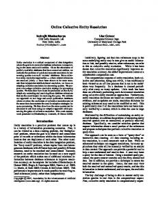
Figure 1: Schematic overview of example MR program execution using 1 map process, m=2 map tasks, 2 reduce processes, and r=3 reduce tasks. In this example, partitioning is based on the key’s color only and grouping is done on the entire key.
entities to distribute the Cartesian product evaluation evenly across all reduce tasks. • We evaluate our strategies and thereby demonstrate their efficiency for learning-based entity resolution with MR. The evaluation is done on a real cloud environment and uses real-world data (Section 4). In the next section, we introduce some preliminaries on MapReduce and learning-based entity resolution. Related work is reviewed in Section 5 before we conclude.
2. 2.1
PRELIMINARIES MapReduce
MapReduce (MR) is a programming model designed for parallel data-intensive computing in cluster environments with up to thousands of nodes [9]. Data is represented by key-value pairs and a computation is expressed with two user defined functions: map : (keyin , valuein ) → list(keytmp , valuetmp ) reduce : (keytmp , list(valuetmp )) → list(keyout , valueout ) These functions contain sequential code and can be executed in parallel on disjoint partitions of the input data. The map function is called for each input key-value pair whereas reduce is called for each key keytmp that occurs as map output. Within the reduce function one can access the list of all corresponding values list(valuetmp ). Besides map and reduce, a MR dataflow relies on three further functions. First, the function part partitions the map output and thereby distributes it to the available reduce tasks. All keys are then sorted with the help of a comparison function comp. Finally, each reduce task employs a grouping function group to determine the data chunks for each reduce function call. Note that each of these functions only operates on the key of key-value pairs and does not take the values into account. Keys can have any arbitrary structure and data type but need to be comparable. The use of extended (composite) keys and an appropriate choice of part, comp, and group supports sophisticated partitioning and grouping
behavior and will be utilized in one of our strategies (see Section 3.2). For example, the center of Figure 1 shows an example MR program with two map tasks and three reduce tasks. The map function is called for each of the four input keyvalue pairs (denoted as �) and the map phase emits an overall of 10 key-value pairs using composite keys (Figure 1 only shows keys for simplicity). Each composite key has a shape (circle or triangle) and a color (light-gray, dark-gray, or black). Keys are assigned to three reduce tasks using a partition function that is only based on a part of the key (“color”). Finally, the group function employs the entire key so that the reduce function is called for 5 distinct keys. The actual execution of an MR program (also known as job) is realized by an MR framework implementation such as Hadoop [1]. An MR cluster consists of a set of nodes that run a fixed number of map and reduce processes. For each MR job execution, the number of map tasks (m) and reduce tasks (r) is specified. Note that the partition function part relies on the number of reduce tasks since it assigns key-value pairs to the available reduce tasks. Each process can execute only one task at a time. After a task has finished, another task is automatically assigned to the released process using a framework-specific scheduling mechanism. The example MR program of Figure 1 runs in a cluster with one map and two reduce processes, i.e., one map task and two reduce tasks can be processed simultaneously. Hence, the only map process runs two map tasks and the three reduce tasks are eventually assigned to two reduce processes.
2.2
Learning-based Entity Resolution
Entity resolution (ER) can be considered as a classification problem. For all entity pairs p ∈ R × S of two input sources R and S, a classifier determines if the entity pair is either a match or a non-match. State-of-the-art ER approaches employ machine learning algorithms to train and apply appropriate classifiers. Machine learning libraries (e.g, Weka) ship with implementations of many classifiers, e.g., Decision Tree (DT) or Support Vector Machines (SVM). Classifiers usually provide standardized interfaces and thus allow for an easy integration into ER workflows. Figure 2 shows a schematic overview of such a learning-based ER workflow that is divided in two phases: classifier training and classifier application. The training phase requires training data, i.e., entity pairs that are annotated whether they represent a match or a non-match. The manual labeling of training data is very time consuming and is typically done offline. Each labeled pair of the training data is annotated with similarity values computed by k different matchers. Based on these pair-wise similarity values and the match/non-match label, a classifier is trained, i.e., a machine learning algorithm generates an internal classification model, e.g., a decision tree. During the second phase the classifier is applied to all relevant entity pairs. In general, ER exploits the Cartesian product of R and S, i.e., the classifier is applied to all possible entity pairs. However, blocking techniques [3] might be employed to reduce the overall number of classifier invocations by pruning entity pairs that are likely to be a nonmatch based on some blocking criteria. The same k matchers as before are utilized to annotate each pair with similarity values before classifier invocation. The pair-wise similarities serve as features for the classification and the classifier
Figure 2: Schematic overview of a learning-based entity resolution workflow.
returns either match or non-match. The final match result typically includes matching entity pairs only, i.e., all “missing” pairs are implicitly considered as non-matches.
3.
SIMILARITY COMPUTATION STRATEGIES
As our analysis will show, the similarity computation in the application phase is by far the most time-critical step. The entire learning phase usually accounts for less than 5% of the overall run-time due to the fact that the training data is significantly smaller than the number of pairs in the application phase. Furthermore, the second phase is dominated by the similarity computation (see Section 4.2). In the following, we therefore focus solely on the efficient pair-wise similarity computation, i.e., applying k matchers to all entity pairs. More specifically we concentrate on the Cartesian product R × S though our approaches can also be employed in conjunction with blocking, i.e., for a subset of R × S. To this end, we propose two strategies that are capable to efficiently distribute all relevant entity pairs across multiple tasks and, thus, perform similarity computation and classifier application in parallel. Both approaches rely on the fact that for any entity pair both similarity computation and classifier application are independent from other entities. The first strategy, MapSide, makes use of the existing data partitioning during the map phase and implements similarity computation solely in the map phase. The second strategy, ReduceSplit, evenly distributes entity pairs across all available reduce tasks that eventually apply matchers for similarity computation.
3.1
MapSide
MapSide makes use of the existing data partitioning during the map phase and implements similarity computation solely in the map phase. It follows the broadcast join idea [5] that “broadcasts” the smaller relation to all map tasks. All map tasks read and buffer the smaller source (R) in memory at initialization time. In the following, the map tasks operate only on the larger source (S) and compare the currently
Figure 3: Example dataflow of the MapSide strategy for m=3 map tasks. The smaller source R is used as additional input for all map tasks.
processed entity of S with all buffered entities. Herewith, the time required for MapReduce-specific data redistribution, sorting, and grouping can be saved. By splitting the smaller source in x blocks and executing the basic strategy x times, MapSide can still be utilized if the smaller source does not entirely fit into main memory. Figure 3 shows an example for a small source R (2 entities) and a larger source S (6 entities). Entities a, b ∈ R are sent to all map tasks as additional input and compared to all data partitions of S, i.e., {c, d}, {e, f }, and {g, h}.
3.2
ReduceSplit
The ReduceSplit strategy realizes the similarity computation during the reduce phase. It targets an even workload distribution across all reduce tasks, i.e., all reduce tasks should process the same number of entity pairs. ReduceSplit follows the idea that both data sources are split into disjoint blocks, i.e., R is split in x blocks and S is split in y blocks. All x blocks of R are compared with all y blocks of S. To this end, ReduceSplit combines composite map output keys with specific partitioning and grouping functions to ensure that all entity pairs are processed and all reduce tasks process (nearly) the same number of entity pairs. During the map phase, ReduceSplit emits y key-value pairs for each entity of R and x key-value pairs for each entity of S. The map key consists of the following three elements: • i = block index of R • j = block index of S • entity’s data source (R or S) For each entity of R, map first assigns a block index i ∈ [0, x − 1]. This can either be done at random or by an enumeration scheme. It then outputs y key-value pairs (i.j.R, entity.R) for j ∈ [0, y − 1]. Analogously, every entity of S is assigned a fixed block index j and x key-value pairs (i.j.S, entity.S) are emitted (i ∈ [0, x − 1]). The structure of the composite key ensures that every entity is compared to all blocks of the other source. Since the number of block pairs usually exceeds the num-
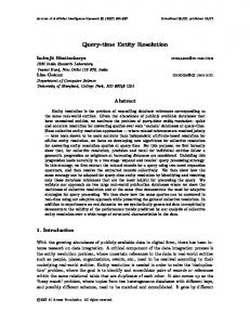
Figure 5: Overall execution time for the MapSide strategy (n=10 nodes, m=100 map tasks) and breakdown into three categories. The number of employed matchers varies from 1 to 6 (see Figure 6 for detailed match configuration).
4. 4.1 Figure 4: Example dataflow of the ReduceSplit strategy for m=3 map tasks and r=3 reduce tasks. Source R is split into x=2 blocks; S in y=3 blocks.
ber of reduce tasks r, a partitioning function part(i, j) = i + j · x
mod r
is applied to distribute the processing of block pairs across all reduce tasks. The partitioning function thereby enumerates all pairs (i + j · x) and assigns them to the reduce tasks consecutively (using the modulo function). The grouping function groups together all map keys sharing the same pair of block indexes. Finally, the keys are sorted and the reduce function can access the values rowby-row. Since the source’s name is part of the composite key, all entities of R appear before all entities of S. The reduce function can therefore buffer all entities of R and then process the following list of entities of S step-by-step, i.e., compare one entity of S with all buffered entities of R. Figure 4 illustrates an example dataflow for the same sources we have already used in Figure 3. Source R is split into x=2 blocks and S is divided into y=3 blocks. For example, entity a ∈ R is assigned a block index i = 0 and emitted y=3 times with the following keys: (0.0.R), (0.1.R), (0.2.R). Entity a is eventually sent to all r=3 reduce tasks and compared to all y=3 blocks of S, i.e., {c, f }, {e, h} , and {d, g}. The main advantage of ReduceSplit over MapSide is that it does not require that one source (R) fits entirely into main memory. Any reduce tasks needs to buffer |R|/x entities only. This benefit comes at the expense of an increased data replication. The map phase emits |R| · y + |S| · x key-value pairs whereas MapSide only replicates (the smaller) source R for each map task, i.e., |R| · m. For |R| < |S| the number of blocks x should therefore be minimized to avoid unnecessary data replication by using the available main memory to full capacity. Furthermore, the resulting x · y block pairs should be evenly distributed across all reduce tasks. Therefore x · y should be a multiple of r.
EVALUATION Experimental Setup
We ran our experiments on Amazon EC2 with up to 50 High-CPU Medium instances in EU West location. Each of these instances runs an Ubuntu 10.04 Server 32-bit OS and provides 1.7GB memory and 5EC2 compute units (2 virtual cores). Both master daemons for managing the distributed file system and the execution of MR jobs ran on a dedicated additional Standard Small instance. Each node was configured to run at most two map and reduce tasks in parallel. On each node, we set up Hadoop 0.20.2. We made the following changes to the Hadoop default configuration: (1) We set the block size of the DFS to 128MB, (2) disabled DFS block replication, (3) allocated 1GB to each Hadoop daemon and (4) 500MB virtual memory to each map and reduce task. (5) Task trackers were allowed to reuse the JVM after task execution for subsequent tasks and (6) speculative execution was turned on. (7) Finally, we increased the sort buffer to 200MB. We utilized two bibliographic datasets that have already been used in previous ER evaluations [19]. DBLP contains about 2,600 entities and the second dataset (Scholar) contains about 64,000 entities. We applied the classifier on each pair of the Cartesian product DBLP× Scholar (168.1 million pairs). For the classifiers, we utilized Weka 3.6.4. In particular, we used a decision tree1 and a SVM2 implementation.
4.2
Time distribution and match quality
In our first experiment, we evaluate the runtime and match quality for different matcher configurations using our MapSide strategy. To this end, we utilize up to six matchers that operate on two attributes (publication title and authors) and apply a decision tree and a SVM for classification, respectively. We vary the number of matchers that are applied before classifier application to illustrate the impact on both the overall execution time and match quality. Figure 5 shows the overall execution time along with a breakdown into similarity computation, classifier application, and remaining MR overhead. Obviously, the overall execution time is clearly dominated by the similarity computation for both classifiers. Depending on the number of matchers, the similarity computation consumes between 88% (one matcher) and 97% (all six matchers) of the runtime. In general, we observe a similar behavior for both 1 2
weka.classifiers.trees.LMT (default parameters) weka.classifiers.functions.LibSVM (linear kernel function)
Figure 6: Average match quality (F-measure) for different classifiers and numbers of matchers.
classifiers. However the application of the SVM appears to be slightly faster. The similarity computation utilizes three similarity measures (TFIDF, Trigram, Jaccard) and two attributes (title and authors) leading to 6 different matchers (see caption of Figure 6). Matchers #1 and #4 are the most expensive since they require an IDF-index3 lookup for each token (i.e., attribute term). Hence, adding matcher #4 leads to a higher increase in computation time than adding other matchers. Furthermore, the length of the author attribute is significantly shorter than of the title attribute. This is especially true for Scholar that suffers from many missing author attribute values. Therefore, adding matchers #5 and #6 only slightly increases the execution time in comparison to matchers #2 and #3. We also evaluate the resulting match quality in our experiment. Figure 6 depicts the F-Measure that is determined based on a (manually created) perfect match result. Since the match quality heavily depends on the quality of training data, we applied the same evaluation strategy as in [19]. For each classifier and matcher combination, we selected 10 times 500 pairs according to the Ratio strategy with a threshold of 0.4 and a ratio of 0.4 using TFIDF similarity and averaged the resulting F-measure over the 10 runs. The results show that employing multiple matchers generally increases the overall match quality. This is especially true if additional matchers operate on different attributes. For example, F-measure increases by 3% to 4% when adding matcher #4. On the other hand, adding too many matchers may deteriorate the match quality due to overfitting (e.g., decision tree for 6 matchers). However, the benefit of multiple matchers underlines the importance of an efficient parallel similarity computation. The decision tree classifier outperforms the SVM by about 2% in F-Measure. On the other hand, the SVM seems to be more stable against an unfavorably matcher selection. Slightly better results have been reported for the same dataset [19], so we expect that match quality can be further increased by tuning the (internal) SVM parameters.
4.3
MapSide vs. ReduceSplit
In a second experiment, we evaluate the efficiency of our two strategies MapSide and ReduceSplit. We use a fixed cloud environment consisting of n = 10 nodes and employ all six matchers. 3 The IDF-Index was computed once with MR as a preprocessing step and is not included in the execution times. The index is stored in the format produced by Hadoops’s MapFileOutputFormat and shipped to each node with Hadoop’s Distributed Cache.
(a) MapSide
(b) ReduceSplit
Figure 7: (a) Execution times for MapSide using varying number m of map tasks. (b) Execution times for ReduceSplit using different numbers x and y of blocks for the two sources DBLP and Scholar, respectively.
Figure 7a shows the resulting execution times for the MapSide strategy for varying numbers of map tasks m = k · 20 (for 1 ≤ k ≤ 5). A higher number of tasks, of course, increases the MR overhead but reduces computational skew effects that stem from matching attribute values of different length and from heterogeneous hardware. Since the similarity computation dominates the overall execution time, computational skew is a serious factor. For example, the overall execution time could be reduced by 20% when increasing m from 20 to 100. For ReduceSplit, we set a fixed the number of map and reduce tasks (m=20, r=20). This is because ReduceSplit already deals with computational skew by defining x · y block pairs that are evenly assigned to the available reduce tasks. We vary both x and y from 1 to 20 and Figure 7b illustrates the resulting execution times for all combinations. In general, we make the following three observations. First, for x · y < r the execution is significantly slow because the cluster is not fully utilized. Second, the experiments prove that x (the number of blocks of the smaller source DBLP) should be smaller than y (the number of blocks of the larger source Scholar). For example, (x=5, y=20) performs better than (x=20, y=5) because in the latter case the larger dataset Scholar needs to be replicated 20 times. Third, increasing y while holding x (x < y) constant usually decreases the execution time because the influence of computational skew is diminished. The only exception is (x=10, y=10) and (x=10, y=15) since the first configuration leads to 100 block pairs that can be evenly distributed across all r=20 reduce task whereas the latter suffers from an uneven distribution because 150 (=number of block pairs) is not a multiple of 20. We repeated the experiment with x, y ∈ [1, 100]. For larger x, y values, we observed relatively constant execution times indicating that load balancing and computational skew aspects are more important than the amount of replicas. The best ReduceSplit configuration (x=5, y=20) in our experiment performs slightly faster than MapSide. However, setting appropriate values for x and y is a difficult task and might depend on the number of reduce tasks as well as the dataset characteristics. We therefore propose to prefer MapSide if the smaller dataset fits into memory.
4.4
Scalability
In our last experiment we prove the scalability of our MapSide realization of learning-based ER. To this end, we vary the number of nodes from n=1 to n=50 and set the number
tokens, or terms) per object to avoid the computation of the Cartesian product. MR groups together objects sharing (at least) one signature and performs similarity computation within the reduce phase. However, these approaches are not adequate for the Cartesian product because they would force one single reduce tasks to perform the entire computation.
6.
Figure 8: Execution times and speedup for all six matchers using 1 up to 50 nodes. of map tasks to m = 10 · n to diminish computational skew effects. Figure 8 shows the resulting execution times and speedup values. We observe an almost linear speedup for up to 10 nodes. Furthermore, we still achieve very good speedup values for up to 50 nodes, e.g., a speedup of 39 for 50 nodes. However, the speedup increase alleviates for more than 10 nodes. This is mainly caused by the fact that an increasing number of map tasks decreases the workload (number of entity comparisons) per map task. At the same time, the relative fraction of the MR overhead for task initialization and task shutdown is increasing. For example, the average execution time per map task for n=10 is about 10 minutes whereas for n = 50 it is about 2 minutes while the (absolute) MR overhead per task remains constant.
5.
RELATED WORK
Entity resolution is a very active research topic and many approaches have been proposed and evaluated [20]. Current state-of-art approaches employ learning techniques to automate matcher configuration and combination. Prior work has considered a variety of classifiers [4, 6]. There are only a few approaches that consider parallel entity resolution. The authors of [7] show how the match computation can be parallelized among available cores on a single node. Parallel evaluation of the Cartesian product of two sources is described in [15]. [16] proposes a generic model for parallel entity matching based on general partitioning strategies that take memory and load balancing requirements into account. There are also first approaches to employ MR for ER (e.g., [22, 23, 18, 17]) but we are not aware of any approaches utilizing MR to speed up learning-based ER. Most work on distributed learning and data mining [14] is about specialized approaches to speed up or parallelize individual learning algorithms. More general approaches are restricted to shared memory machines [13]. First approaches of scalable machine learning algorithms using MR are Mahout [2], SystemML [11] or [8]. However, much of this work reverts back to hand-tuned implementations of specific algorithms on MapReduce or is proprietary. MR-based similarity computation has recently gained interest for many domains. Example applications include pairwise document similarity [10] to identify similar documents, join computation [5] in relations, and set-similarity joins [22] for efficient string similarity computation. All approaches generate one or more signatures (e.g., join attribute values,
SUMMARY AND OUTLOOK
We studied how learning-based entity resolution can be realized efficiently with MapReduce. We thereby identified that the similarity computation of the Cartesian product is the dominant factor and proposed two different MapReducebased strategies for this task. Our evaluation shows that our strategies are able to distribute the similarity computation and classifier application among the available computational resources and scale with the number of nodes. In future work, we will extend our approaches to incorporate blocking strategies and load balancing approaches to handle computational skew. Another approach to further reduce computation time is to analyze the learned model in order to prune similarity computation for pairs that are unlikely to match.
7.
REFERENCES
[1] Hadoop. http://hadoop.apache.org/mapreduce/. [2] Mahout. http://mahout.apache.org/. [3] Baxter et al. A comparison of fast blocking methods for record linkage. In Workshop Data Cleaning, Record Linkage, and Object Consolidation, 2003. [4] Bilenko and Mooney. Adaptive duplicate detection using learnable string similarity measures. In ACM SIGKDD, pages 39–48, 2003. [5] Blanas et al. A comparison of join algorithms for log processing in mapreduce. In SIGMOD, pages 975–986, 2010. [6] Chaudhuri et al. Example-driven design of efficient record matching queries. In VLDB, pages 327–338, 2007. [7] Christen et al. Febrl - a parallel open source data linkage system. In PAKDD, pages 638–647, 2004. [8] Chu et al. Map-reduce for machine learning on multicore. In NIPS, pages 281–288, 2006. [9] Dean and Ghemawat. MapReduce: Simplified Data Processing on Large Clusters. In OSDI, 2004. [10] Elsayed et al. Pairwise Document Similarity in Large Collections with MapReduce. In ACL, 2008. [11] Ghoting et al. SystemML: Declarative machine learning on mapreduce. In ICDE, pages 231–242, 2011. [12] Hall et al. The weka data mining software: an update. SIGKDD Explorations, 11(1):10–18, 2009. [13] Jin et al. Shared memory parallelization of data mining algorithms: Techniques, programming interface, and performance. IEEE Trans. Knowl. Data Eng., 17(1):71–89, 2005. [14] Kargupta et al. The distributed data mining bibliography. URL http://www. csee. umbc. edu/˜ hillol/DDMBIB, 2011. [15] Kim and Lee. Parallel linkage. In CIKM, pages 283–292, 2007. [16] Kirsten et al. Data partitioning for parallel entity matching. In QDB, 2010. [17] Kolb et al. Multi-pass Sorted Neighborhood Blocking with MapReduce. CSRD, pages 1–19, 2011. [18] Kolb et al. Parallel Sorted Neighborhood Blocking with MapReduce. In BTW, 2011. [19] K¨ opcke et al. Evaluation of entity resolution approaches on real-world match problems. PVLDB, 3(1), 2010. [20] K¨ opcke and Rahm. Frameworks for entity matching: A comparison. Data Knowl. Eng., 69(2), 2010. [21] Mierswa et al. Yale: Rapid prototyping for complex data mining tasks. In SIGKDD, pages 935–940, 2006. [22] Vernica et al. Efficient parallel set-similarity joins using MapReduce. In SIGMOD, 2010. [23] Wang et al. MapDupReducer: Detecting near duplicates over massive datasets. In SIGMOD, 2010.