Learning Causal Graph: A Genetic Programming ... - Semantic Scholar

International Journal of Machine Learning and Computing, Vol. 4, No. 3, June 2014

Learning Causal Graph: A Genetic Programming Approach Amer Bakhach and Mahmoud Samad 1

Abstract—Representing causal relation between set of variables is a challenged objective. Causal Bayesian Networks has been classified as good modeling technique for this purpose. However structure learning for causal Bayesian networks still suffering from several problems including the causal interpretation of the model and the complexity of the learning algorithm. In this research the author presents an approach for learning causal graph based on Wiener-Granger causal-theory, with minor modifications, and use Genetic Programming to determine the parameters of Granger formula. This approach enjoys necessary advantages: reasonable complexity and cover nonlinear equation. A case study of 5 global stock markets is presented to experimentally explain and support this approach. The finding show that SP500 has Granger-causal influence on NIKKE: the accuracy of forecasting NIKKE stock market can be incremented by 24% when integrating past data from SP500. Whereas Euro STOXX 50 is reported to be the least stock Granger-causally affected by the others. Index Terms—Genetic programming, granger-causality, learning causal graph, stock market forecasting, JEL classification: G15 – C32 – D83.

I. INTRODUCTION Traditional Bayesian Network (BN) has been used dozens of times to model relation between variables. However the interpretation of these relations differs; for example [1], [2] claim that their Direct Acyclic Graph (DAG) reflects causal relation whereas others (e.g. [3], [4]) argue that causality in traditional BN structure is not that obvious. A clear statement is cited in [4]: “Formally Belief Networks only make independence statements, not causal ones,” One important reason for why BN can not imply causation is that most of used structure learning approaches are based on information score metrics such as: BDe, K2, MIT. etc. [5]; those metrics discover correlation between variable. More precisely they measure the degree of association between each variable and its parent variables in the network; but correlation does not imply causation [6]. In other words, Bayesian Network can be interpreted as probabilistic model that reflect relation like conditional independence and associational relationship but without consideration of causality. Causal Bayesian networks was introduced with the intention to solve the problem of “causal” interpretation. It’s simply based on the instinct that everything occurred according to some reason(s) (i.e. cause). Its importance is evident since the decisions concluded based on causal model Manuscript received August 7, 2013; revised December 30, 2013. Amer Bakhach and Mahmoud Samad are with the Computer Sciences Department, Lebanese International University, Lebanon (e-mail: [email protected], [email protected]).

DOI: 10.7763/IJMLC.2014.V4.419

243

are more significant, and more reliable. Finally causal inference is much more likely to be achieved rather than traditional inference because it allows us to predict the effects of interventions in a domain. Two researchers are recognized as leaders in “causality definition and modeling”: a) Pearl ([7] and [8]) subsumes and unifies many approaches of causation, and provides a consistent mathematical foundation for the analysis of causes and counterfactuals, and b) Granger [9], the Nobel Prize winner in economic sciences, is well-known for his researches on causality especially in econometrics. According to Granger: to detect causal effect of a variable X on variable Y we should measure how much integrating past data of X can improve the forecasting the present value of Y. Most of recent works addressing causation are based on the works of at least one of these two researchers. However the definition of causality and its interpretation in causal Bayesian networks is still a challenge. For instance reference [3] describes a Bayesian Approach to learning causal networks; and [10] propose a method for learning causal Bayesian network structures from experimental data using MCMC-based model. Definition and interpretation of causality in these two works simply does not match. This paper introduces a new technique for learning causal graph, but not necessary a Direct Acyclic Graph (DAG), based on Wiener-Granger causality theory. Since Grangercausality is compatible with most other definitions of causality, it has been widely accepted. This work mainly refer to the original papers of Wiener [11] and Granger [9]; however two modifications on Granger equations will be described practically. The parameters of Granger equations will be estimated via Genetic Programming (GP). We also explain how GP can solve problem of nonlinear equation. We use the Mean Square Error (MSE) as fitness function for GP. Based on MSE, we define and calculate Level of Significance (LS) of causal influence to deduce edges’ orientations. Case of nonlinear equation is covered using GP. The accompanied case study is composed of 5 global stock markets: SP500, EURO STOXX 50, CAC 40, FTSE 100, and NIKKE225. The goal is to discover the associated Granger-causal graph to these stocks. The rest of this paper proceeds as follow: Section II provides a brief review of Bayesian network and causal Bayesian network; Section III describes the basic concept of Wiener and Granger-causal theory and describe my proposed modifications; Section IV explains the essentials of Genetic Programming and its advantages for this research; in Section V explains briefly how to construct a causal graph structure according to this approach; Section VI provides a case study of five global stock markets with deep details. Some related works are listed in Section VII; we

International Journal of Machine Learning and Computing, Vol. 4, No. 3, June 2014

conclude in Section VIII.

III. WIENER-GRANGER CAUSALITY WITH MINOR MODIFICATION A. Granger Causality In its simplest explanation Granger-Causality (GC) measures an associational relation between the historical of a variable and the current of another based on the intuitive supposition that a cause have to happened before its result. The basic idea was introduced by Wiener [11]: if the accuracy of forecasting the current value of given time series variable X is enhanced by integrating past values of another time series Y then Y is said to have causal influence on X. Wiener’s idea was not supported by mathematical formulas or explanation that make it practical. Granger [9] formalized the necessary calculus in the framework of linear regression models. Specifically, “if the variance of the autoregressive prediction error of the first time series at the present time is reduced by inclusion of past measurements from the second time series, then the second time series is said to have a causal influence on the first one,” More formally: Let X and Y are two time series data and let Ut be all the data in the universe collected since time t-1 and let Ut-Yt denote all this data without the indicated time series Yt: The following definitions are adopted from [9]; let σ2 (X|Y) denote the predictive error variance of Xt using only the past of Yt. Definition 1: Causality. If σ2 (X|U) < σ2 (X|U-Y), we say that Y is causing X, denoted by Yt→ Xt. Definition 2: Feedback. If σ2 (X|U) < σ2 (X|U-Y) and σ2 (Y|U) < σ2 (Y|U-X) that is: feedback is said to occur when Xt is causing Yt and also Yt is causing Xt. As consequence a causal graph may not being “acyclic” in such case. Let’s consider the following simplified equations of two variable case:

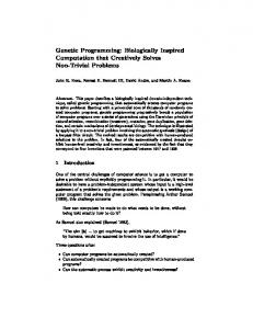
II. BAYESIAN NETWORKS AND CAUSAL BN A. Bayesian Networks Bayesian Networks (BN) [2] is a graphical modeling technique that is based on the assumption of the existence of relationships among different included variables. BN graph is a direct acyclic graph (DAG) that shows, mainly, the structure of relationship of dependency, associational relationship and conditional independency (as edges) between different variables (as nodes), see Fig. 1. DAG structure can be determined either from historical data (structure learning) or by an expert (or even by combination of both). Next, conditional probability tables (CPT) are constructed. The model finally can be used for inference purposes. At many works, edges are assumed to have causal implication; but they could not prove this assumption although some researchers try to do so (e.g. [12]-[14]); they end up that having a causal interpretation of BN can be very important [3]. In the matter of fact most BN structure are constructed based on score metrics approaches that rely on information theory (e.g. Mutual Information, Entropy). The main problem with information theory is that it mainly discover correlation and not causation which is simply a different subject. Reference [3] called that type of networks “a causal Bayesian networks” and basically it represents probabilistic independence. Our concern in this study is the causal implication of edges in a graph; which is the corner stone of causal Bayesian network. B. Causal Bayesian Networks The advantage of causal model over probabilistic model, e.g. BN, is clarified in [15]:

∑ ∑

“Causal model are much more informative than probability models. A joint distribution tells us how a probable events are and how probabilities would change with subsequent observations, but a causal model also tell us how these probabilities would change as a result of external interventions (e.g. treatment management). These changes cannot be deduced from a join distribution even if fully specified,”

+ E1(t) ∑

(1) + E2(t)

(2)

In the original theory of Granger [9], lags length are assumed to be equal (i.e. m =q.) E1(t) and E2(t) are the prediction errors for each time series. Now if it’s found that error of (2) is significantly lower than (1) then we say that Y Granger-cause X. More details on measurement of “significance” is given in next paragraph. The solution of how to determine the parameters ai and bj will be given in next section according to this approach.

For simplicity we denote by causal Bayesian network a couple consisting of a directed acyclic graph (called causal DAG) that stand for causal relationships and a set of probability tables, that in association with the graph identify the joint probability of the variables represented as nodes in the graph. More formal definition of causal Bayesian networks can be found in [15]. In this paper we focus on one perspective only: causal interpretation of edges in a causal DAG.

B. Minor Modifications In this work we applied two basics modifications on the Granger-causality concept described in previous paragraph: 1) Lag length First, in this work m can be different, i.e. not equal, from q in (2). Logically, the assumption of m=q does not hold always in reality. Simply put, let us assume that m=1, that is x is perfectly predicted using xt-1 value; there is no reason to conclude from this that yt-2 can not contribute efficiently in predicting xt. The results of [16] is an experimental approval that it is normal to have m≠q in a Granger-causal test. In addition, reference [17] show that the results of Grangercausality tests are extremely sensitive to the lag condition.

Fig. 1. Sample direct acyclic graph (DAG).

244

International Journal of Machine Learning and Computing, Vol. 4, No. 3, June 2014

We conclude from this that dealing with lags in VAR model need more attention. In reality selecting the lag length of VAR model can be problematic. Several methods for calculating lag length were described in [18]. According to this approach, in the notation of the above augmented regression (2), m is the shortest, and q is the longest, lag length for which the lagged value of x is significant. Calculating m and q is discussed in Section VI.

original linear version of the theory, described above, and we will explain how to cover the limitation of nonlinearity by using GP in next section. The potential of relying on Granger-causality come from its compatibility with most other notions of structure learning and causality. For example the link between information theory and Granger causality has been reviewed in [23]: they discuss the conceptual and theoretical relations between Granger causality and directed information theory; and report that “measures based on directed information theory naturally emerge from Granger causality inference frameworks,” In addition, it was proved in [24] that Pearl’s Causal Model and Granger causality are in fact closely linked. Furthermore, Granger-causal theory outperforms many other approaches for exploring causal relationships as reported in [25].

2) MSE instead of error variance Another difference exists between theory of Granger and this approach. In this work we measure forecasting error using the Mean Square Error (MSE) (3) instead of the error variance σ2. We suppose that replacing σ2 with MSE in definition 1 and 2 does not affect the accuracy of Grangertheory; i.e. definitions 1 and 2 still holds using MSE. This assumption is based on: a) The MSE includes together the variance of the estimator and its bias and b) in regression analysis, the MSE is consistent although it is not an unbiased estimator of the error variance, and c) MSE is, clearly, well-matched with initial concept of Wiener causaltheory [11]. MSE

∑

Ŷi-Yi)2

IV. GENETIC PROGRAMMING Genetic Programming is based on Darwin’s theory of evolution: “survival of the fittest,” It starts with a generation composed of set of computer programs that will reproduce with each other for thousands of iterations. At each iteration, the finest programs only stay alive then they replicate with each other’s again to compose the next generation and so on. Theoretically each generation, i.e. set of programs, should perform better than its predecessors [26]. The main concept is that any mathematical equation can be modeled as a tree. See for example, Fig. 2.a and Fig. 2.b. Hence the problem is to find the optimal equation; i.e. optimal tree. GP objective is to find this tree.

(3)

where Ŷ and Y are two vectors of n predicted values and true values respectively. Hence, the MSE evaluates the quality of a predictor in terms of its variation (σ2) and degree of bias (4). MSE (Ŷ) = σ2(Ŷ )+ Bias ((Ŷ ,Y))2

(4)

That is we compute MSEX and MSEX|Y for equations (1) and (2) respectively. Next, we define a so-called variable Level of Significance (LSX|Y) used in this work to measure how much integrating past data from Y will increase the accuracy of predicting X. LSX|Y (in %) is counted as follow (5): (5) Note: LSx|y =0 only if MSEx = MSEx|y; that is only if knowing x does not improve the predictability error of y. The roles of the two variables X and Y, in equation (1) and (2), can then be overturned to test the existence of causal influence in the reverse direction. One important note is that none of these two modifications violate the original causal theory according to Wiener [11]. Using Granger-causality test is common especially in economics, see for example [19] and [20]. Recently combining the concept of Granger causality with graphical models has become very attractive [21]. As can be noticed from [9] the associated definitions (1 & 2) make no assumptions on the data generation process. However the supposition of linearity in VAR-based Gcausality does not hold always in reality. Although extension for non-linear cases have been made (see for example [22]), but in this paper we adopt the

Fig. 2.a. tree expression of equation M+ [(K*L) /X]

Fig. 2.b. tree expression of equation (a/b)* Log M

Fig. 2.c. tree expression of equation a/b+ [(K*L) /X]

Fig. 2.d. equation M* Log M

To this end GP proceed as follow: a. Randomly generate a set S of N equations, i.e. trees, similar to Fig 2.a. & Fig 2.b., where N could be several hundred (or thousands). This is the first generation of equations b. Sort the equations in S according to a fitness function (e.g. MSE) c. Select TOP M equations (where M is a parameter that can be set by user.) 245

International Journal of Machine Learning and Computing, Vol. 4, No. 3, June 2014

d.

New generation is to be formed by reproduction, using crossover and mutation (more details after few lines). e. Step d should end up with another N equations, which form the new S. Hypothetically, new S will contain better equation(s), i.e. tree(s), than the previous set. f. If stop criterion =false then Go to step b else quite In step b, The fitness function is necessary in order to be capable to algorithmically decide whether one solution; i.e. tree; is better than another. In step d, we can mate any two equations by randomly exchanging subtrees that compose them to yield children; i.e. equations that have the same elements as their parents. For example of crossover, the two trees Fig. 2.c and Fig. 2.d. are children of the two at the top. Practically, the same two parents might equally well produce a large number of other offspring. Crossover make guaranty that GP is not limited to linear equations, see Fig. 2.d. for example. More details on advantages of using GP for nonlinear system can be found in [27]. As can be seen, the previous algorithm assures the convergence to the global optimal solution; although it may not reach it. Due to “mutation,” in step d, falling in local optima is avoided. Mutation can be defined, from GP perspective, as a sudden alteration in a specific node; for example: assume in Fig. 2.d the root node can become “/” instead of “*”; the expression turn out to be: M / Log M. Criterion to stop the running can be defined such as: a) a threshold of error (e.g. MSE < β) or b) number of generation without significance improvement in fitness function (e.g. 2000 successive generations without improvement of MSE). According to Wiener-Granger causal-theory, we are not interested in finding the exact equations’ parameters; instead we are more concerned with accuracy of level of significance (LS). That is by computing MSE with high accuracy using GP we can then determine LS easily. In my approach we rely on GP to estimate parameters, ai and bi, of Granger formulas (1) and (2) as well the lag value m & q (more details on this is given in the accompanied case study). The advantage of using optimization algorithm, such GP, is to attain a computational advantage (see [28] for details) over many other graphical Granger methods those could be computationally too expensive to be applicable in some cases such as: Exhaustive Granger [20]. Other advantages of GP are: its results are human readable, the automatic selection of variables, and it cover nonlinear equation easily. GP has been a main technique for many researches in time series forecasting and modeling (see for example [29], [30].)

Building edges in a causal graph depend mainly on value of LS; however if both -LSy|x & LSy|x- are below a specific threshold α, to be defined in next section, then no G-causal effect exist between those two variables and by consequence no edges are drawn. In next section we provide an explicit case study that shows in details the construction of causal graph of five stock markets according to my approach.

VI. CASE STUDY: GLOBAL STOCK MARKET Causality among stock markets has been widely discussed through tens of researches. For instance [1] construct a DAG which assumed to reflect causality among 9 stock markets; causality representation was not confirmed since their method was based on error correction modeling which only reflect interdependency and not causality. Reference [31] introduces a model to infer the volatility of the data, to be used in risk management, while explicitly accounting for dependencies between different companies. However their model can not imply causation; in fact it only takes into concern the existence of relationship of dependency between stock market when calculating the volatility. A. Data Description The used data cover the period from October 21th 2002 to July 12th 2013. In this approach, we will try to discover the existence of causal-relation between each pair of stock markets. Therefore each try will have its own tailored data. More specifically for each pair, X and Y, we include only the common working days. That is if any of the two stocks was off at date t then the record of that date was omitted from this case. Then we measure the fractional change of the obtained data according to (6) for both included stock market X and Y. (

)

Generally, for each case we got more than 2500 instances. (Raw data is available for download at: http://amerbakhach.com/ICMLC2014/data.xls ) The included 5 major stock markets are: SP500, EURO STOXX 50, CAC 40, FTSE 100, and NIKKE 225. B. Example of Granger-Causality Detection between SP500 and NIKKE Based on (1) and (2) let’s suppose that X is NIKKE and Y is SP500, in order to determine if SP500 G-cause NIKKE we get the following equations: ∑

V. BUILDING G-CAUSAL GRAPH VIA GP

∑

Constructing G-causal graph can be done as following: First: For each pair of time series- X and Y- find LSx|y and LSy|x using GP. Second:  if (LSy|x ≈ LSy|x) than we fall into case of feedback (Definition 2).  if LSy|x > α then build an edge from x to y.

(6)

+ E1(t) ∑

(7) +E2(t) (8)

C. Discipulus: A Software for Genetic Programming As previously explained in Section IV, GP is an optimization algorithm that can determine the parameters of (7) and (8). Discipulus is easy-to-use commercial software that applies GP. Discipulus has a feature called self-tuning 246

International Journal of Machine Learning and Computing, Vol. 4, No. 3, June 2014

and self-parameterizing which selects the GP control parameters based on its problem to be solved [32], [33]. It has been used in many researches as a GP tool (see for example [34].) In addition Discipulus provide other useful information such as:  MSE: for each resulted equation generated by Discipulus, it count the associated Mean Square Error (MSE) of the equation. we use the MSE as fitness function.  Once the software marque no improvement in fitness function; i.e. MSE; for several generations; it restart the whole procedure again. This help in avoiding falling in local optima.  Input impact: for each variable, e.g. NIKKEi and SPj in (7) & (8), it calculate its coefficient which is defined as its importance for determining the predicted variable NIKKEt. This is very useful to conclude the Lag values; i.e. m & q; in 7 & 8. More specifically Discipulus count three numbers for each input variable: Frequency, Average Impact (AI), and Maximum Impact (MI) ;

where AI and MI show, respectively, the average and the maximum effect of removing that input from each of the thirty best programs, i.e. trees, and replacing it with a permuted version of that input [33]. By comparing these three numbers for each variable it become easy to determine m and q.

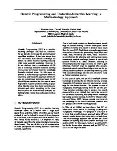
D. Significance Threshold (α) We define a threshold variable α as the limit to draw an edge based on LS; that is if LSx|y ≥ α then an edge must be drawn from y to x. For example, according to results from previous paragraph, if α = 10 we obtain Fig. 3.a.

NIKKE 10.43 -24.41

FTSE 7.87 14.98 ---

CAC 7.58 7.27 5.42

EURO STOXX 5.39 24.57 5.33

CAC 40 EURO STOXX 50

6.97

0

0.5

---

2.1

0.06

6.72

0

0.36

---

Fig. 4.a. causal graph with α = 7

F. Note for experiment At each causal test and for each pair of stocks, we should recalculate all MSEs because data is synchronized according to each pair. (See the data file at http://amerbakhach.com/ICMLC2014/data.xls .) In other words, the test for each pair is assumed to be completely independent. For example when testing Granger-causality between CAC and FTSE we got MSECAC=1.989 whereas when we do the same test between CAC and EURO we got MSECAC=2.198.

VII. RELATED WORKS

NIKKE

Fig. 3.a. causal graph with α = 10 (Feedback case)

SP -24.3 11.58

In reference [10] the authors did not prove the compatibility of their model with neither Pearl nor Granger; in fact they only try to clarify some rules of when a BN can be interpreted as causal BN. Although they claim that their approach can discover causal edges with area under curve (AUC) approaching 95%. One important approach was given in [35]. They express an influence diagram, which is familiar for representing decision problem [4], in a canonical form and prove its ability to represent causal relation, and its compatibility with Pearl’s causal-theory as well [8]. They explain how causal BN can be extracted from this influence diagram. Reference [3] proposes an extension for Bayesian methods those were used to learn acausal Bayesian network to learn causal Bayesian network; always respecting Pearl’s causal-theory. Reference [16] present work very similar to this research in term of testing Granger-causality between stock markets. However the difference is that the author did not use Genetic Programming and no causal-graph was constructed

whereas if α = 15 we obtain Fig. 3.b.

NIKKE

Stock markets SP500 NIKKE 225 FTSE

Fig. 4.b. causal graph with α = 10

The result is: MSENIKKE (7) = 2.255 and MSENIKKE|SP500 (8) = 1.707; thus LSNIKKE|SP500= 24.3 %. Next we reverse the order of SP500 and NIKKE in equations (7) & (8) we got: MSESP = 1.486 and MSESP|NIKKE= 1.331 and hence LSSP|NIKKE= 10.43%.

SP500

TABLE I: LS (X|Y): X STOCKS IN FIRST COLUMN, AND Y STOCKS IN FIRST ROW

SP500

Fig. 3.b causal graph with α = 15

E. Global Stock Market Causal Graph By following instructions in paragraph B. for each pair of stocks, we got the following result summarized in Table I. The results in table can be interpreted as follow: integrating past data of EURO STOXX 50 will increase the accuracy of forecasting NIKKE 225 by 24.57% while integrating past data from NIKKE improve forecasting of EURO STOXX only by 6.72%. Therefore we can conclude that for α>7 EURO STOXX G-cause NIKKE while the reverse is not true. Resulted causal graph with α = 7 and α = 10 in Fig. 4.a and Fig. 4.b respectively. 247

International Journal of Machine Learning and Computing, Vol. 4, No. 3, June 2014

neither. Finally, they adopt the lag condition m=q which may not be realistic as discussed previously in section III. In addition, other works provide methods for constructing causal graph based on Granger theory; however, some of these methods are computationally infeasible such as: exhaustive graphical Granger and the SIN Granger method; while some, in order to reduce the complexity, make assumptions that may threat the generalization of original causality implication such as SIN Granger method and VAR method. Note that the computational complexity is a key issue that affects the feasibility of a learning algorithm since in real world we may deal with large-scale data [36]. Although GP may not, in some cases, reach the optimal solution, i.e. tree, but it enjoy desirable features such as very acceptable complexity since you can stop the process anytime, in comparison to other methods, and it does not make any further assumptions; hence the main concept of Granger-causality [9] is conserved using GP, and finally there is no need to assume the existence of linear Gaussian model as in VAR method. And finally it solve the nonlinearity problem without additional complexity in contrast to many other models [27], [28], [36].

networks, and Prof. Yves Rakotodratsimba (ECE Paris) for his advices in financial analysis. REFERENCES [1]

[2] [3]

[4] [5]

[6]

[7]

[8]

[9]

VIII. CONCLUSION AND PERSPECTIVES [10]

This paper presents a simple, yet advantageous, technique to construct causal graph based on Granger-causal theory. This was also the objective of many other researches. The main difference is that this approach use Genetic Programming (GP) to compute all parameters of Grangercausality equations. we select G-causality because it enjoys several advantages like: compatibility with information theory, and Pearl causal model. However we provide two modifications on lag length and error variance; we prove that the first is necessary in reality while the second dose not affect the validity of Granger-causal theory. we choose GP because of its desirable advantages: acceptable computation, convergence to global optimal solution is guaranteed, and cover case of nonlinearity. In addition GP allow us to overcome the condition of equal length (m=q) in Granger VAR-equations; since such condition is not realistic in many cases. The case study provides detailed practical experiment for data from stock markets. The finding shows that NIKKE is the most Granger-causally affected stock market whereas EURO STOXX is the least causally affected. While CAC show a neutron G-causal effect at α ≥ 8. Since BN has been used for stock markets prediction [37], we believe that this approach for causal graph learning can improve the accuracy prediction of stock markets; in addition causal inference according to this approach should be investigated. This approach does not take into concern the possible existence of dynamic causality. In other words the calculated values of LS may vary over time. Further research may address this subject.

[11]

[12]

[13]

[14]

[15] [16]

[17]

[18] [19]

[20]

[21]

[22]

[23]

ACKNOWLEDGMENT [24]

The authors would thanks Dr. Iyad Zaarour, from Lebanese university, for his useful hints on Bayesian 248

D. A. Bessler and J. Yang, “The structure of interdependence in international stock markets,” Journal of International Money and Finance, vol. 22, pp. 261–287, 2003. A. Darwiche, Modeling and Reasoning with Bayesian Networks Cambridge University Press, 2009, ch. 1 pp. 9 & ch. 4, pp. 63-70. Heckerman. “A Bayesian approach to learning causal networks,” in Proc. Eleventh Conference on Uncertainty in Artificial Intelligence, Quebec, 1995, pp. 285-295. D. Barber, Bayesian Reasoning and Machine Learning, Cambridge University Press, 2012, ch. 3, pp. 47 & ch.7, pp. 127-130. L. M. de Campos, “A Scoring Function for Learning Bayesian Networks based on Mutual Information and Conditional Independence Tests,” Journal of Machine Learning Research, vol. 7 pp. 2149-2187, 2006. Novella. (2009). Evidence in Medicine: Correlation and Causation. Science and Medicine. Science-Based Medicine. [Online]. Available: http://www.sciencebasedmedicine.org/index.php/evidencein-medicine-correlation-and-causation/ J. Pearl, “Bayesianism and Causality, or, Why I am Only a HalfBayesian” Foundations of Bayesianism (Applied Logic Series), vol. 24, pp 19-36, December 2001. J. Pearl. (1995). Causal diagrams for empirical research. Biometrika. [Online]. 82(4). pp. 669-688. Available: http://biomet.oxfordjournals.org/content/82/4/669.abstract C. W. J. Granger. “Investigating causal relations by econometric models and cross-spectral methods,” Econometrica, vol. 37, no. 3, pp. 424–438, 1969. B. Ellis and W. H. Wong, “Learning causal bayesian network structures from experimental data,” Journal of the American Statistical Association, vol. 103, no. 482, pp. 778-789, June 2008. N. Wiener, “The theory of prediction,” in Modern Mathematics for Engineers, E. F. Beckenbach, Ed. New York: McGraw-Hill, 1956, vol. 1. J. Pearl and T. Verma. “A theory of inferred causation,” in Knowledge Representation and Reasoning: Proceedings of the Second International Conference, J. Allen, R. Fikes, and E. Sandewall, Eds. New York, 1991, pp. 441–452. M. J. Druzdzel and H. A. Simon. “Causality in Bayesian belief networks,” in Proc. the Ninth Annual Conference on Uncertainty in Artificial Intelligence, San Francisco, CA, 1993, pp. 3-11. D. Margaritis, “Learning bayesian network model structure from data,” Ph.D. dissertation, School of Computer Science, Carnegie Mellon University, May 2003. J. Pearl, Causality Models, Reasoning and Inference, 2nd edition, Cambridge University Press, 2009, ch. 1, pp. 21-25 B. Comincioli. (1996). The stock market as a leading indicator: an application of granger causality. The Park Place Economist. [Online]. 4. Available: http://digitalcommons.iwu.edu/parkplace/vol4/iss1/13 D. L. Thornton and D. S. Batten. (1984). Lag length selection and granger causality. Working Paper Series 1984-001A Federal reserve bank of St. Louis. [Online]. Available: http://research.stlouisfed.org/wp/1984/1984-001.pdf F. Canova, Methods for Applied Macroeconomic Research, Princeton University Press, 2007, ch. 4, pp. 110-113. P. Foresti. (April 2007). Testing for Granger causality between stock prices and economic growth MPRA Paper No. 2962. [Online]. Available: http://mpra.ub.unimuenchen.de/2962/1/MPRA_paper_2962.pdf S. H. Chen, C. H. Yeh, and C. C. Liao, “Testing for granger causality in the stock price-volume relation: a perspective from the agent-based model of stock markets,” in Proc. International Conference on AI, 1999, pp. 374-380 M. Eichler “Graphical modeling of multivariate time series,” Probability Theory and Related Fields, vol. 153, issue 1-2, pp. 233268, June 2012. N. Ancona, D. Marinazzo, and S. Stramaglia, “Radial basis function approaches to nonlinear Granger causality of time series,” The American Physical Society- Physical Review E 70, 056221, 2004. P. Amblard and O. J. J. Michel. “The relation between granger causality and directed information theory: a review,” Entropy, vol. 15, pp. 113-143, 2013. H. White, K. Chalak, and X. Lu, “Linking granger causality and the pearl causal model with settable systems,” JMLR: Workshop and Conference Proceedings, 2011, vol. 12, pp. 1-29.

International Journal of Machine Learning and Computing, Vol. 4, No. 3, June 2014 [36] A. Arnold, Y. Liu, and N. Abe “Temporal causal modeling with graphical granger methods,” in Proc. the 13th ACM SIGKDD international conference on Knowledge discovery and data mining, 2007 CA, USA, pp. 66-75 [37] E. Kita, Y. Zuo, M. Harada, and T. Mizuno “Application of Bayesian Network to stock price prediction,” Artificial Intelligence Research, vol. 1, no. 2, December 2012.

[25] C. Zou, C. Ladroue, S. Guo, and J. Feng. (2010). Identifying interactions in the time and frequency domains in local and global networks a Granger causality approach. BMC Bioinformatics. [Online]. 11. pp. 337. Available: http://www.biomedcentral.com/content/pdf/1471-2105-11-337.pdf [26] J. Koza, Genetic programming: On the programming of computers by means of natural selection, Cambridge, MA: MIT Press, 1992, ch. 6. [27] A. Patelli “Genetic Programming Techniques for Nonlinear Systems Identification,” PhD dissertation, Universităţii Tehnice Gheorghe, Romania, 2011 [28] B. Rylander, T. Soule, and J. Foster “Computational Complexity, Genetic Programming, and Implications,” Lecture Notes in Computer Science, vol. 2038, pp. 348-360, 2001. [29] S. Chen and C. Yeh, “Using genetic programming to model volatility in financial time series,” in Proc. Genetic Programming 1997: the Second Annual Conference, 1997, pp. 288-306. [30] M. Santini and A Tettamanzi, “Genetic Programming for Financial Time Series Prediction,” in Proc. the 4th European Conference on Genetic Programming London, 2001, pp. 361-370. [31] C. Hendahewa and V. Pavlovic, “Analysis of Causality in Stock Market Data,” in Proc. the 2012 11th International Conference on Machine Learning and Applications, vol. 01, pp. 288-293. [32] F. D. Francone. (2010). Discipulus Owner Manual. [Online]. Available:http://www.rmltech.com/doclink/Owners%20Manual/Disci pulus_Owners_Manual.pdf [33] J. A. Foster, “Review: discipulus: a commercial genetic programming system,” Genetic Programming and Evolvable Machines, vol. 2, issue 2, pp. 201-203, June 2001. [34] N. Priyadharshini and M. S. Vijaya, “Genetic programming for document segmentation and region classification using discipulus,” International Journal of Advanced Research in Artificial Intelligence, vol. 2, no. 2, pp. 15-22, 2013. [35] D. Heckerman and R. Shachter, “A decision-based view of causality,” in Proc. the Tenth Conference on Uncertainty in Artificial Intelligence. Seattle, 1994, pp. 302-310.

Amer Bakhach received a diploma in teaching from Lebanese Ministry of higher education in 2002 and a master degree MBA-management information system in 2008 from Jinan University, Lebanon. In 2010 he received his master degree of computer sciences-bioinformatics from Lebanese University. He held multiple position in industry as web development and IT manger (all in Lebanon) from 2003-2009. Since October 2009 he has been a member of Lebanese International University as lecturer in computer sciences department. Currently interested on Bayesian network and its application in finance and bioinformatics.

Mahmoud Samad received his BS degree in 2003, MS degree in 2005 and PhD in computer sciences from University of Toulouse 3, France in 2009. He is currently an assistant professor in Computer Science Department at the Lebanese International University, Lebanon. His main topics of interest are large-scale distributed systems and graphical models.

249