Learning Investment Functions for Controlling The Utility of Control. Knowledge .... a rule head, the set of subgoals of the rule body, under the current binding, is given to ... A under all the solutions of B. For each subgoal Ai, its average cost is ...
Learning Investment Functions for Controlling The Utility of Control � Knowledge Oleg Ledeniov and Shaul Markovitch Computer Science Department Technion { the Israel Institute of Technology Haifa, Israel
Abstract
The utility problem occurs when the cost of the acquired knowledge outweighs its bene�ts. When the learner acquires control knowledge for speeding up a problem solver, the bene�t is the speedup gained due to the better control, and the cost is the added time required by the control procedure due to the added knowledge. Previous work in this area was mainly concerned with the costs of matching control rules. The solutions to this kind of utility problem involved some kind of selection mechanism to reduce the number of control rules. In this work we deal with a control mechanism that carry very high cost regardless of the particular knowledge acquired. We propose to use in such cases explicit reasoning about the economy of the control process. The solution includes three steps. First, the control procedure must be converted to anytime procedure. Second, a resource-investment function should be acquired to learn the expected return in speedup time for additional control time. Third, the function is used to determine a stopping condition for the anytime procedure. We have implemented this framework within the context of a program for speeding up logic inference by subgoal ordering. The control procedure utilizes the acquired control knowledge to �nd e cient subgoal ordering. The cost of ordering, however, may outweigh its bene�t. Resource investment functions are used to cut-o� ordering when the future net return is estimated to be negative.
Introduction
Speedup learning is a sub-area of machine learning where the goal of the learner is to acquire knowledge for accelerating the speed of a problem solver (Minton 1988� Tadepalli & Natarajan 1996). Several works in speedup learning concentrated on acquiring control knowledge for controlling the search performed by the problem solver. When the cost of using the acquired control knowledge outweighs its bene ts, we face the so called Utility Problem (Minton 1988� Gratch & DeJong 1992� Markovitch & Scott 1993). Existing works dealing with the utility of control knowledge are based on a model of control rules whose Submitted to AAAI-98
main associated cost is the time it takes to match their preconditions. Several solutions has been proposed for this instance of the utility problem. Most of the solutions are based on ltering out control rules that are estimated to be of low utility (Minton 1988� Markovitch & Scott 1993� Gratch & DeJong 1992). Others try to restrict the complexity of the preconditions (Tambe, Newell, & Rosenbloom 1990). In this work we deal with a di�erent setup where the control procedure has potentially very high complexity regardless of the speci c control knowledge acquired. In this type of setup, the utility problem can become very signi cant since the cost of using the control knowledge can be very high { higher than the time it saves on search. Filtering is not useful for such cases, since deleting control knowledge will not necessarily reduce the complexity of the control process. We propose to use a three step framework for dealing with this problem: 1. Convert the control procedure into anytime program. 2. Learn the resource investment function for the anytime procedure. This function predicts the expected saving in search time for given resources invested in control decision. 3. Run the anytime control procedure such that the control time plus the expected search time will be minimal. This framework is demonstrated through a learning system for speeding up logic inference. The control procedure is our Divide-and-conquer algorithm. The learning system learns costs and number of solutions of subgoals to be used by the ordering algorithm. A \good" ordering of subgoals will increase the e�ciency of the logic interpreter. However, the ordering procedure has very high complexity. We employ the above framework by rst converting our Divide-and-conquer algorithm to anytime procedure. We then learn a resource investment function for each goal pattern. The functions are then used to terminate the ordering procedure before its costs become too high. We demonstrate experimentally how the ordering time decreases
without harming signi cantly the quality of the resulting order.
Learning control knowledge for speeding up logic inference
In this section we describe our learning system which performs o�-line learning of control knowledge for speeding up logic inference. The problem solver is a Prolog interpreter for pure Prolog. Thus the goal of the learning system is to speed up the SLD-resolution search of the AND-OR tree.
The control procedure
The control procedure orders AND nodes of the ANDOR search tree. When the current goal is uni ed with a rule head, the set of subgoals of the rule body, under the current binding, is given to our Divide-and-conquer algorithm to nd a low-cost ordering. The algorithm produces candidate orderings and estimates their cost using the following equation: Cost A1 A2 : : :An i) = Pn (hP jb ) = i =1 h b2Sols(fA1 :::A ;1 g) Cost(Ai� Pn Qi;1 (1) i=1 j =1 nsols(A�j )jfA1 :::A ;1 g � cost(Ai )jfA1:::A ;1 g : where cost(A)jB is the average cost of proving a subgoal A under all the solutions of a set of subgoals B and nsols(A)jB is the average number of solutions of A under all the solutions of B. For each subgoal Ai , its average cost is multiplied by the total number of solutions of all the preceding subgoals. The main idea of the Divide-and-conquer algorithm is to create a special AND-OR tree, called the divisibility tree, which represents the partition of the given set of subgoals into subsets, and to perform a traversal of this tree. The partition is performed based on dependency information. We call two subgoals that share a free variable dependent. A leaf of the tree represents an independent set of subgoals. An AND node represents a subset that can be partitioned into subsets that are mutually independent and each of the AND branches corresponds to the divisibility tree of one of the partitions. An OR node represents a dependent set of subgoals. Each OR branch corresponds to an ordering where one of the subgoal in the subset is placed rst. The selected rst subgoal binds some of the variables in the remaining subgoals. For each node of the tree, a set of candidate orderings is created, and the orderings of an internal node are obtained by combining orderings of its children. For di�erent types of nodes in the tree, the combination is performed differently. We prove several su�cient conditions that allow us to discard a large number of possible ordering combinations, therefore the obtained sets of candidate orderings are generally small. The candidate orderings are propagated up the divisibility tree. The last step of the algorithm is to return the lowest cost candidate i
j
i
of the root according to equation 1. In most practical cases the new algorithm works in polynomial time. For more details about the Divide-and-conquer algorithm see (Authors 1998).
The learning component
The learning system performs o�-line learning by generating training queries according to the same distribution as the previous user queries. The ordering algorithm described above assumes the availability of correct values of average cost and number of solutions for various literals. The learning component acquires this control knowledge while solving the training queries. Storing a separate unit of control values for each literal is not practical, for several reasons. The rst is the large space required by this approach. The second reason is the lack of generalization: the ordering algorithm is quite likely to encounter literals which were not seen before, and whose real control values are thus unknown. The learner therefore acquires control values for classes of literals rather than for separate literals. The more re ned are the classes, the smaller is the variance of real control values inside each class, the more precise are the cost and nsols estimations that the classes assign to their members, and the better orderings we obtain. One easy way to de ne classes is by modes or binding patterns (Debray & Warren 1988� Ullman & Vardi 1988): for each argument we denote whether it is free or bound. Class re nement can be obtained by using more sophisticated tests on the predicate arguments than the simple \bound-unbound" test. For this purpose we can use regression trees { a sort of decision trees that classify to continuous numeric values (Breiman et al. 1984� Quinlan 1986). Two separate regression trees are stored for every program predicate, one for its cost values, and one for the nsols. For each literal whose cost or nsols is required, we address the corresponding tree of its predicate and perform recursive descent in it, starting from the root. Each tree node contains a test which applies to the arguments of the literal. Since we store separate trees for di�erent predicates, we do not need tests that apply to the predicate names. A possible regression tree for estimation of number of solutions for predicate father is shown on Figure 1. The tests used in the nodes can be syntactic, like the following examples: � Is the rst argument bound? � Is the rst argument the constant c1? � Is the rst argument greater than 80? � Is the rst argument greater than the second one? They can also be semantic: � Is the rst argument male? � Is the rst argument the father of the second one?
Average: 10 Test: bound(arg1)?
yes
no
Average: 0.5 Test: female(arg1)?
yes Average: 0.0
Average: 50 Test: bound(arg2)?
no
yes
Average: 0.8 Test: bound(arg2)?
yes Average: 0.001
Average: 1.0
no Average: 100
no Average: 2.0
Figure 1: A regression tree for estimation of number of solutions for father(arg1,arg2).
� Is the rst argument married to some relative of the
second argument? � Is the rst argument older than the second one? If we only use the test \is argument i bound?", then the classes of literals de ned by regression trees coincide with the classes de ned by binding patterns. Semantic tests require logic inference. For example, the rst one of the semantic tests above invokes the predicate male on the rst argument of the literal. Therefore these tests must be as \cheap" as possible, otherwise the retrieval of control values will take too much time.
Subgoal ordering and the utility problem
To test the e�ectiveness of our ordering algorithm, we experimented with it on various domains, and compared its performance to other ordering algorithms. Most experiments were performed on randomly created arti cial domains. We also tested the performance of the system on several real domains. Most experiments described below consist of a training session, followed by a testing session. Training and testing sets of queries are randomly drawn from a xed distribution. During the training session the learner acquires the control knowledge for literal classes. During the testing session the problem solver proves the queries of the testing set using di�erent ordering algorithms. The goal of ordering is to reduce the time spent by the Prolog interpreter when it proves queries of the testing set. This time is the sum of the time spent by the ordering procedure (ordering time) and the time spent by the interpreter (inference time). In order to ensure statistical signi cance of results of comparison of di�erent ordering algorithms, we experimented with many di�erent domains. For this purpose, we created a set of arti cial domains, each with a small xed set of predicates, but with random number of clauses in each predicate, and with random rule lengths. Predicates in rule bodies, and arguments in
both rule heads and bodies are randomly drawn from xed distributions. Each domain has its own training and testing sets (these two sets do not intersect). Since the domains and the query sets are generated randomly, we repeated each experiment 100 times, each time with a di�erent domain. The following ordering methods were tested: � Random: Each time we address a rule body, we order it randomly. � Best-�rst search: over the space of pre xes. Out of all pre xes that are permutation of each other, only the cheapest one is retained. A similar algorithm was used Markovitch and Scott (1989). � Adjacency: A best- rst search with adjacency restriction test added. The adjacency restriction requires that two adjacent subgoals always stands in the cheapest order. A similar algorithm was described by Smith and Genesereth(1985). � The Divide-and-conquer algorithm using binding patterns for learning. � The Divide-and-conquer algorithm using regression trees with syntactic tests. Table 1 shows the results obtained. The results clearly show the advantage of the Divide-and-conquer algorithm over other ordering algorithms. It produces much shorter inference time than the random ordering method. It requires much shorter ordering time than the other deterministic ordering algorithms. Therefore, its total time is the best. The results with regression trees are better than the results with binding patterns. This is due to the better accuracy of the control knowledge that is accumulated for a more re ned classes. It is interesting to note that the random ordering method performs better than the best- rst and the adjacency methods. The inference time that these method produce is much better than the inference time when using random ordering. However, they require very long ordering time which outweighs the inference time gain. This is a clear manifestation of the utility problem where the time required by the control procedure outweighs its bene t. The Divide-and-conquer algorithm has much better ordering performance. however, its complexity is O(n!) in the worst case. Therefore, it is quite feasible to encounter the utility problem even when using the e�cient ordering procedure. To study this problem, we performed another experiment where we varied the maximal length of rules in our randomly generated domains and tested the e�ect of the maximal rule length on the utility of learning. Rules with longer bodies require much longer ordering time, but also carry a large potential bene t. The graph on Figure 2 plots the average time saving of the ordering algorithm: for each domain we calculate the ratio of its total testing time with the Divide-andconquer algorithm and with the random method. For
Ordering Uni cations Reductions Ordering Inference Total Ord.Time Method Time Time Time Reductions Random 86052.06 27741.52 8.191 27.385 35.576 0.00029 Best- rst 8526.42 2687.39 657.973 2.933 660.906 0.24 Adjacency 8521.32 2686.96 470.758 3.006 473.764 0.18 Divide-and-conquer 8492.99 2678.72 8.677 2.895 11.571 0.0032 - binding patterns Divide-and-conquer 2454.41 859.37 2.082 1.030 3.112 0.0024 - regression trees Table 1: The e�ect of ordering algorithm on the tree sizes and the CPU time (mean results over 100 arti�cial domains). Literal classes for control computations are de�ned by binding patterns.
Average utility ratio 1
Average time ratio
0.8
These results show that risk of encountering the utility problem exists even with our e�cient ordering algorithm. In the following section we present a methodology for controlling the cost of the control mechanism by explicit reasoning about its expected utility.
Controlling the utilization of control knowledge
0.6
0.4
0.2
0 2
4
6 Maximal rule body length
8
10
Figure 2: The graph of average utility ratios for various maximal rule body lengths.
each maximal body length, a point on the graph shows the average over 50 arti cial domains. For each domain, testing with the random method was performed 20 times, and the average result was taken. The following observations can be made: 1. For short rule bodies, the Divide-and-conquer ordering algorithm performs only a little better than the static random method. When bodies are short, little permutations are possible, thus the random method often nds good orderings. 2. For middle-sized rule bodies, the utility of the Divide-and-conquer ordering algorithm grows. Now the random method errs more frequently (there are more permutations of each rule body, and less chance to pick a cheap permutation). At the same time, the ordering time is not too large yet. 3. For long rule bodies, the utility again decreases, and the average time ratio nearly returns to the 1.0 level. Although the tree sizes are now reduced more and more (compared to the sizes of the random method), the additional ordering time grows notably, and the overall e�ect of ordering becomes almost null.
The last section showed an instance of the utility problem which is quite di�erent from the one caused by the matching time of control rules. There, the cost associated with the usage of control knowledge could be reduced by ltering out rules with low utility. Here, the high cost is an inherent part of the control procedure and is not a direct function of the control knowledge. For cases such as the above, we propose to use a a methodology with the following three steps: 1. Convert the control procedure to an anytime algorithm. 2. Acquire the resource-investment function for the algorithm that predicts the expected reduction in search time as a result of investing more control time. 3. Execute the anytime control procedure with a termination criterion that is based on the resource investment function. In this section, we will show how this three-step methodology can be applied to our Divide-and-conquer algorithm.
Anytime Divide-and-conquer algorithm
The Divide-and-conquer algorithm propagates the set of all candidate orderings in a bottom-up fashion to the root of the divisibility tree. Then it uses Equation (1) to estimate the cost of each candidate and nally returns the cheapest candidate. The anytime version of the algorithm works di�erently: � Find rst candidate, compute its cost. � Loop until a termination condition holds (and while there are untried candidates): { Find next candidate, compute its cost.
{ If it is cheaper than the current minimal one {
update the current cheapest candidate. � Return the cheapest candidate out of all seen till now. In the new framework, we do not generate all candidates exhaustively (unless the termination condition never holds). This algorithm is an instance of anytime algorithm (Boddy & Dean 1989� Boddy 1991): it always has a \current" answer ready, and at any moment can be stopped and return its current answer. The new algorithm visits each node of the divisibility tree several times: it nds its rst candidate, then pass this candidate to higher levels (where it participates in mergings and concatenations). Then, if the termination condition permits, the algorithm re-enters the node, nds its next candidate and exits with it, and so on. The algorithm stores for each node a information about the last candidate created. Note that all the nodes of a divisibility tree never physically co-exist simultaneously, since in every OR-node only one child is maintained at every moment of time. Thus, if the termination condition occurs in the course of the execution, some OR-branches of the divisibility tree are not created.
Using Resource-Investment Functions For Termination Control
The only part of the above algorithm that remains unde ned is the termination condition which dictates when the algorithm should stop exploring new candidates and return the currently best candidate. Note that if this condition is removed or is always false then all candidates are created, and the anytime version becomes equivalent to the original Divide-and-conquer algorithm. The more time we dedicate to ordering, the more candidates we create, and the cheaper becomes the best current candidate. This functional dependence can be expressed by a resource-investment function (RIF for shorthand). execution time texe
optimal point
secure stop
ordering time tord
Figure 3: A resource-investment function. An example of a RIF is shown on Figure 3: the x-axis (tord ) corresponds to the ordering time spent, small cir-
cles on the graph are candidate orderings found, and the y-axis (texe ) shows the execution time of the cheapest candidate seen till now (the execution time includes the inference time of the rule itself, and all the inference and ordering time that will be spent on the lower levels of the proof tree). The function decreases when a cheaper candidate is seen, and it never grows. After we see the globally cheapest candidate, the RIF becomes constant. For each point (candidate) on the RIF, we can de ne the total computation time which is the sum of the ordering time it takes us to reach this point and the time it takes to execute the currently cheapest candidate: tall = tord + texe (2) There exists a point (candidate) for which this sum is minimal(\optimal point" on Figure 3). This is the best point to terminate the anytime ordering algorithm: if we stop before it, execution time of the chosen candidate will be large, and if we stop after it, the ordering time will be large. In each of the two cases the total time spent on this rule will increase. Thus, the termination condition of our anytime algorithm can be expressed as follows: TerminationCondition :: OptimalPoint(candidate) But how can we know that the current point on the RIF is optimal? We have only seen the points before it (to the left of it), and cannot predict how the RIF will behave further. If we continue to explore the current RIF until we see all the candidates (then we surely can detect the optimal point), all the advantages of an early stop are lost. We cannot just stop at the point where tall starts to grow, since there may be several local minima of tall . However, there is a condition that guarantees that optimal point can not occur in the future. if the current ordering time tord becomes greater than the currently minimal tall , there is no way that the optimal point will be found in later stage, since tord can only grow thereafter, and texe is positive, tall cannot become smaller than the current minimum. So using this termination condition guarantees that the current known minimum is the global minimum. It also guarantees that, if we stop at this point, the total execution time will be: opt topt ord + 2 � texe opt where (topt ord texe) are the coordinates of the point with minimal tall (the \optimal point" on Figure 3). Now the total time is less than twice the optimal one. We can maintain a variable topt all and update it after the cost of a new candidate is computed. The termination condition therefore becomes: TerminationCondition :: tord topt (3) all where tord is the time spent in the current ordering. The point where these two value become equal is shown as the \secure stop" point on Figure 3.
Experimentation
We have implemented the anytime algorithm, with both terminal conditions 3 and 4. In the following experiments, the ordering method which uses the former de nition of the terminal condition (3) is called the current-RIF method, and the second one (4) is called the learned-RIF method. We rst repeated the rst experiment of Section with the following three conditions: 1. No limitations are set on the ordering algorithm (termination condition is always false). 2. Current-RIF: The ordering algorithm stops at the secure stop point (termination condition de ned by Equation 3). 3. Learned-RIF: The ordering algorithm stops at the estimated optimal point (termination condition dened by Equation 4).
Uncontrolled ordering Controlled ordering
1
0.8
Average time ratio
Although the secure-point-stop strategy promises us that no more than twice the minimal e�ort is spent, we would surely prefer to stop at the optimal point. A possible solution is to learn the optimal point, basing on RIFs produced on the previous orderings of this rule. This learning can be conducted, for example, by a classi cation tree, where attributes are rule head arguments, and tests are the same as were proposed for regression trees of cost computation. Before we start ordering a rule, we use the learned tree to estimate the optimal stop point for this rule. Assume that this point is at time topt . Then the termination condition for the anytime algorithm is TerminationCondition :: tord topt (4) where tord is the time spent in the current ordering. One problem with both formulas 3 and 4 is that they use CPU time. It is much more convenient and safe to work with discrete measurements. In the same way as we introduced cost units as a discrete analogue of the execution time (e.g., the number of uni cations performed), we can de ne ordering units that re�ect the number of steps performed by the ordering procedure (e.g., the number of nodes visited or candidates created). In addition, we cannot know exactly how long it will take us to execute a candidate ordering {we can only estimate its cost according to our control knowledge (and Equation 1). Therefore, we must introduce two transformation coe�cients: � one to translate the number of ordering units (from the start of ordering and until now) into ordering time that passed, � one to translate estimated cost of an ordering into estimated execution time. These two values can be learned from experience. We can assume that for a given program and a given query distribution these coe�cients do not change signi cantly.
0.6
0.4
0.2
0 2
4
6 Maximal rule body length
8
10
Figure 4: The graph of average utility for various maximal rule body lengths.
The results are shown in Table 2. As we see, the tree sizes did not change signi cantly. But the number of ordering units is decreased drastically (divided by 5 if we explore current RIF, and by 10 if we learn RIFs). The average time of ordering one rule (the rightmost column of the table) also decreased strongly, which shows that much less ordering is performed, and this does not lead to worse ordering results (large tree sizes). We next repeated the second experiment described in Section , distributing domains by their maximal body lengths, and computing the average utility of the ordering algorithm separately for each maximal body length. The upper graph on Figure 4 is the same as on Figure 2 from Section , where we performed complete ordering. The new graph is shown in dotted line, and corresponds to ordering with anytime algorithm (using learned RIFs for estimating the optimal stop point). We can see that using the resource-sensitive ordering algorithm reduced eliminated the utility problem by controlling the costs of ordering long rules.
Conclusions
This paper presents a technique for dealing with the utility problem when the complexity of the control procedure that utilizes the learned knowledge is very high regardless of the particular knowledge acquired. We propose to convert the control procedure into anytime algorithm and perform explicit reasoning about the utility of investing additional control time. This reasoning uses the resource investment function of the control process which can be either learned, or built during execution. We show an example of this type of reasoning in a learning system for speeding up logic inference. The system orders sets of subgoals for increased inference e�ciency. The costs of the ordering process, however, may exceed its potential gains. We describe a way to
Ordering Method
Uni cations Ordering Ordering Inference Total Time Ord.Time Units Time Time Reductions complete ordering 2467.95 12817.29 1.668 1.039 2.707 0.001931 current RIF 2338.15 2586.66 0.686 0.999 1.685 0.000833 learned RIFs 2340.37 1279.63 0.569 1.027 1.595 0.000690 Table 2: Comparison of the uncontrolled and controlled ordering methods. convert the ordering procedure to be anytime. We then show how to reason about the utility of ordering using a resource investment function during the execution of the ordering procedure. We also show how to learn and use resource investment functions. The methodology described here can be used also for other domains such as planning. There, we want to optimize the total time spent for planning and execution of the plan. Learning resource investment functions in a way similar to the one described here may increase the e�ciency of the planning process.
References
Authors. 1998. The divide-and-conquer subgoalordering algorithm for speeding up logic inference. Research report, Ommited for con dentiality. Boddy, M., and Dean, T. 1989. Solving timedependent planning problems. In Proceedings of the Eleventh International Joint Conference on Arti cial Intelligence, 979{984. Los Altos, CA: Morgan Kauf-
mann. Boddy, M. 1991. Anytime problem solving using dynamic programming. In Proceedings of the Ninth National Conference on Arti cial Intelligence, volume II, 738{743. Menlo Park: AAAI Press/MIT Press. Breiman, L.� Friedman, J. H.� Olshen, R. A.� and Stone, C. J. 1984. Classi cation and Regression Trees. Wadsworth International Group. Debray, S. K., and Warren, D. S. 1988. Automatic mode inference for logic programs. The Journal of Logic Programming 5:207{229. Gratch, J., and DeJong, D. 1992. COMPOSER: A probabilistic solution to the utility problem in speedup learning. In Proceedings of the Tenth National Conference on Arti cial Intelligence, 235{240. San Jose, California: American Association for Arti cial Intelligence. Markovitch, S., and Scott, P. D. 1989. Automatic ordering of subgoals { a machine learning approach. In
Proceedings of North American Conference on Logic Programming, 224{240.
Markovitch, S., and Scott, P. D. 1993. Information ltering: Selection mechanisms in learning systems. Machine Learning 10(2):113{151.
Minton, S. 1988. Learning Search Control Knowledge: An Explanation-Based Approach. Boston, MA: Kluwer. Quinlan, J. R. 1986. Induction of decision trees. Machine Learning 1:81{106. Smith, D. E., and Genesereth, M. R. 1985. Ordering conjunctive queries. Arti cial Intelligence 26:171{ 215. Tadepalli, P., and Natarajan, B. K. 1996. A formal framework for speedup learning from problems and solutions. Journal of Arti cial Intelligence Research 4:419{443. Tambe, M.� Newell, A.� and Rosenbloom, P. 1990. The problem of expensive chunks and its solution by restricting expressiveness. Machine Learning 5(3):299{348. Ullman, J. D., and Vardi, M. Y. 1988. The complexity of ordering subgoals. In Proceedings of the Seventh ACM SIGACT-SIGMOD Symposium on Principles of Database Systems, 74{81.