Learning Multiple Levels of Representations with Kernel ... - arXiv

Learning Multiple Levels of Representations with Kernel Machines Shiyu Duan 1 Yunmei Chen 2 Jose C. Principe 1

arXiv:1802.03774v2 [cs.LG] 2 Apr 2018

Abstract We propose a connectionist-inspired kernel machine model with three key advantages over traditional kernel machines. First, it is capable of learning distributed and hierarchical representations. Second, its performance is highly robust to the choice of kernel function. Third, the solution space is not limited to the span of images of training data in reproducing kernel Hilbert space (RKHS). Together with the architecture, we propose a greedy learning algorithm that allows the proposed multilayer network to be trained layerwise without backpropagation by optimizing the geometric properties of images in RKHS. With a single fixed generic kernel for each layer and two layers in total, our model compares favorably with state-of-the-art multiple kernel learning algorithms using significantly more kernels and popular deep architectures on widely used classification benchmarks.

1. Introduction We address two issues that are commonly considered to be inherent in kernel PNmachines, i.e., learning machines of the form f ( · ) = i=1 αi k(xi , · ), where N ∈ N, {αi : i = 1, 2, 3, ..., N } ⊆ R and {xi : i = 1, 2, 3, ..., N } ⊆ X are arbitrary, k : X × X → R is a real kernel function. First, kernel machines are unable to learn multiple levels of distributed representations, which has become a source of criticism since such a capability is now generally considered essential for complicated artificial intelligence (AI) tasks. Second, performance of kernel machine is usually highly dependant on the choice of kernel since it governs the quality of the accessible function space in RKHS but few rules or good heuristics exist for that topic due to its task-dependent 1

Department of Electrical and Computer Engineering, University of Florida, Gainesville, Florida, USA 2 Department of Mathematics, University of Florida, Gainesville, Florida, USA. Correspondence to: Shiyu Duan , Jose C. Principe .

nature. Despite the fact that they are capable of universal function approximation (Park & Sandberg, 1991; Micchelli et al., 2006) and that they enjoy a very solid mathematical foundation (Aronszajn, 1950), kernel machines, like many other general-purpose learning machines, are being overshadowed by multilayer neural networks in the most challenging fields of AI such as computer vision, natural language processing, etc. Extensive works have argued for the dominance of neural networks in these fields and it has been widely accepted that, to learn highly complicated functions that are able to represent high-level abstractions required in complex AI tasks, it is highly desirable both from a mathematical perspective and in terms of biological plausiblity that the learning machine can learn multiple levels of distributed representations (Bengio, 2009; LeCun et al., 2015; Mhaskar et al., 2016). Due to architectural constraints, kernel machines do not naturally possess such learning capability. Hence our first contribution is that we bridge this gap between neural networks and kernel machines via building a multilayer network of kernel machines, each layer consisting of an array of kernel machines as units. The network as a whole learns hierarchical, distributed representations via function compositions. To propose a solution to the second issue, we first argue why the choice of kernel matters in practice. It has been well-established that, under the assumption that X is a topological space together with mild conditions on k that are easily met by an infinite number of the prePkernels, N Hilbert space H defined as {f ( · ) = α k(x i, · ) : i=1 i N ∈ N, αi ∈ R, xi ∈ X, i = 1, 2, 3, ..., N }, is dense in the supremum norm in CC (X), the set of all continuous functions with compact support whose domain is X (Park & Sandberg, 1991; Micchelli et al., 2006).1 Further, for a given machine Pn learning task, despite that a kernel machine f ( · ) = i=1 αi k(xi , · ) is only capable of implementing functions in a proper subspace of H due to n and {x1 , x2 , ..., xn } being fixed, the representer theorem 1

Unless it is clear from context or noted otherwise, we always assume that any kernel discussed in this paper meets the conditions for a kernel to be universal (Micchelli et al., 2006), that is, it induces a kernel machine that is capable of universal approximation.

Learning Multiple Levels of Representations with Kernel Machines

(Sch¨olkopf et al., 2001) guarantees that this subspace HS includes the optimal solution f ? to any given regularized empirical risk minimization problem. In practice, however, due to regularization on the function class that is necessary for any learning to happen (Cristianini & Shawe-Taylor, 2000), the set of functions the kernel machine can effectively implement, denoted HS0 , is a strict subset of HS because α1 , α2 , ..., αn can no longer be arbitrary. And f ? normally is not in HS0 . In other words, despite that an infinite number of kernels can be turned into kernel machines that are capable of universal approximation in theory, the choice of k is critical in practice since it governs the “goodness” of the accessible subset HS0 and hence the quality of the regularized solution. Arguably, the most popular approach to tackle this limitation is Multiple Kernel Learning (MKL) (Bach et al., 2004; G¨onen & Alpaydın, 2011), which mitigates the issue via learning a mixture of kernels. In terms of the function space that the resulting kernel machine can effectively utilize, MKL enlarges the accessible function space by combining several RKHS’s in a parametric and usually linear fashion. However, since the RKHS’s induced by many generic kernels are already large enough to contain practically any function, it can be more fruitful and efficient if the learning machine can explore freely a single RKHS without being limited to the span of the images of training data. We show that it is possible to optimize the accessible function space of a kernel machine directly such that the machine can effectively utilize a better subspace of the RKHS than the original in the sense that this subspace contains a better and potentially more efficient approximation to the true target function. For this purpose, we present a layer-wise learning algorithm for the proposed model under a classification setting with an arbitrary number of classes. The algorithm involves only a single feedforward phase and it essentially makes the network learn a kernel matrix one layer at a time. And we will show that the objective of learning is equivalent to driving the images of the given training data in RKHS closer to an orthonormal set with class labels encoded in the directions of vectors. The incentive is that such a distribution of images in RKHS tightens margin-based generalization bounds for linear classifiers (Cristianini & Shawe-Taylor, 2000; Sch¨olkopf & Smola, 2001). And learning is rather robust to the choice of kernel: it suffices to use a single generic kernel with all its hyperparameters fixed. The proposed learning algorithm is similar in spirit to the pioneering work in (Lanckriet et al., 2004). Our contribution is two-fold. First, we provide the geometric interpretations of learning and utilize those insights for training a multilayer network without backpropagation. Second and perhaps more importantly, we show that even with a single completely fixed generic kernel, we can obtain practically

any arbitrary kernel matrix we desire and the optimization need not be constrained to make the resulting kernel matrix positive semidefinite. This contrasts with existing works where the learning usually concerns kernel selection among multiple kernels and has to be formulated explicitly as a constrained optimization problem and many settings of training such as the choice of cost function have to be restricted to accommodate those requirements.

2. A Multilayer Network of Kernel Machines We now describe how we can build a connectionist model from kernel machines. Since we are describing a multilayer network, it is benefitial to establish some nomenclature to avoid confusions: the layer closest to input is called the first layer. And we shall use subscripts to distinguish components within one layer and superscripts for numbering components from different layers. For example, f32 ( · ) denotes the third kernel machine on the second layer. Note that in this paper, we shall only propose the model as well as the learning algorithm for classification with an arbitrary number of classes. 2.1. The Architecture We now describe the architecture of MultiLayer Kernel Network (MLKN). In MLKN, each layer is an array of kernel machines. Take the first layer as an example, its function form can be written as F 1 ( · ) = (f11 ( · ), f21 ( · ),P ..., fd1 ( · )), where for j = 1, 2, 3, ..., d, we n have fj1 ( · ) = i=1 αji k 1 (xi , · ) and αji ∈ R is arbitrary for all admissible j and i, S = {x1 , x2 , ..., xn } ⊆ X is a given random sample. Due to the universality of k 1 and the representer theorem, we know that F 1 ( · ) is a universal approximator for practically any function from X to Rd , where d is the number of kernel machines on the first layer. Or, equivalently, F 1 ( · ) is capable of learning practically any representation of the original random sample in Rd . Given an element xi from S, its new representation would be F 1 (xi ) = (f11 (xi ), f21 (xi ), ..., fd1 (xi )) ∈ Rd . For simplicity, we denote the set {F 1 (x1 ), F 1 (x2 ), ..., F 1 (xn )} as F 1 (S) and will use this shorthand as much as possible. When trained with the greedy learning algorithm that we shall propose in the following subsection, the mapping F 1 ( · ) will be learned by the kernel machines on the first layer in such a way that if the learned representation F 1 (S) are later mapped to a RKHS H 2 by the mapping Φ2 ( · ) defined as Φ2 ( · ) = k 2 ( · , · ), the images Φ2 (F 1 (S)) ⊆ H 2 will form an orthonormal set with the following property: if xi , xj are from the same class, then their images Φ2 (F 1 (xi )), Φ2 (F 1 (xj )) are identical; otherwise, their images are orthogonal. When such a mapping F 1 ( · ) is successfully learned

Learning Multiple Levels of Representations with Kernel Machines

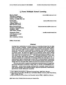
after a new kernel machine f 2 ( · ) = Pn training, 2 1 1 i=1 βi k (F (xi ), F ( · )) is trained to classify the learned representation. In terms of the advantages in classifying with Φ2 (F 1 (S)), first, it is straightforward that Φ2 (F 1 (S)) is always linearly separable in the RKHS H 2 . Furthermore, if k 2 is unsigned with the property k 2 (x, x) = C, ∀x ∈ Rd for some nonzero constant C, then for any two classes from Φ2 (F 1 (S)), the margin with respect to the class of all linear functions in H 2 is no smaller than that of Φ2 (T ), ∀T ⊆ Rd , see Appendix A for a proof. According to (Cristianini & Shawe-Taylor, 2000), this suggests that among all possible representations of S in Rd , the learned representation F 1 (S) is optimal for kernel machine f 2 ( · ) in terms of generalization. This MLKN described above is a two-layer MLKN with the first layer being an array of kernel machines trained for representation learning and the second layer being a new kernel machine trained for classification. Note that one may need multiple kernel machines on the second layer for classification with more than two classes. To construct a MLKN with more layers, instead of training the second layer as a classifier as we did previously, one should repeat the construction and training process of the first layer to build the second layer also as a representation learner. To be specific, one can build another array of p kernel machines F 2 ( · ) = (f12 ( · ), f22 ( · ), ..., fp2 ( · )) that take F 1 (S)Pas input, i.e., for j = 1, 2, 3, ..., p, we have n 2 1 1 fj2 ( · ) = i=1 βji k (F (xi ), F ( · )). Then the entire two-layer model as a whole learns a composed mapping F 2 (F 1 ( · )) = F 2 ◦ F 1 ( · ). And F 2 ( · ) is a universal approximator for practically any function mapping from Rd to Rp by construction. Similar to the first layer, the second layer should learn a mapping such that the new representation F 2 ◦ F 1 (S), when later mapped to the RKHS induced by a new kernel k 3 by the mapping defined as Φ3 ( · ) = k 3 ( · , · ), will be an orthonormal set in that RKHS. When the first and second layers Pnare properly trained, a new kernel machine f 3 ( · ) = i=1 γi k 3 (F 2 ◦ F 1 (xi ), F 2 ◦ F 1 ( · )) is trained for classification. Now we have a three-layer MLKN with the first two layers being a hierarchical representation learner and the third layer being a classifier that works with the learned representation. See Figure 1 for an illustration of the architecture. The same construction can be repeated to obtain more layers. Some remarks addressing how MLKN is different from a traditional kernel machine are in order. First, MLKN learns hierarchical and distributed representations. To see this, first note that, by construction, MLKN is capable of learning multiple levels of representations through function compositions F s ◦ F s−1 ◦ · · · ◦ F 1 ( · ). Also, that any

Figure 1. Illustration for the architecture of a three-layer MLKN. The learning objective for the first two layers is such that, after the random sample S has gone through the learned mappings, which are F 1 ( · ) and F 2 ( · ), the images in a new RKHS of the learned representation of S, written F 2 ◦ F 1 (S), form an orthonormal set with labels (indicated by the color of the arrows) encoded in directions of vectors. The last layer is a kernel machine classifier that works with the representation F 2 ◦ F 1 (S).

internal representation is distributed follows directly from the uniformity in kernel machines within a layer and full connectivity between layers. Further, in Appendix A, we show that just like in neural networks, in-layer uniformity and full inter-layer connectivity will not necessarily result in all kernel machines within a layer learning identical solution functions. Secondly, in each MLKN layer, images of the given random sample S in RKHS under the kernel mapping can be learned whereas, for a traditional kernel machine, they are completely determined by the kernel function. Take the previously described three-layer MLKN for example and consider any kernel machine on the second layer, denoted fj2 ( · ). Naturally, Φ2 ( · ) is fully characterized by k 2 and is fixed during learning, the images of S in H 2 , on the other hand, is Φ2 (F 1 (S)) and hence determined both by Φ2 ( · ) and F 1 ( · ). And F 1 ( · ) is subject to learning. Thus, except for the first layer, images in the RKHS of each layer can be optimized via adjusting weights of kernel machines on the preceding layer. And if we were to view Φ2 (F 1 ( · )) = Φ2 ◦ F 1 ( · ) as a composed kernel mapping, then {Φ2 ◦ F 1 ( · ) : αji ∈ R} is in fact a class of kernel mappings even though we have only introduced a fixed kernel for each of the two layers respectively. It is equivalent to conclude that {k 2 ◦ F 1 ( · , · ) := k 2 (F 1 ( · ), F 1 ( · )) : αji ∈ R} characterizes a class of kernel functions: this justifies why MLKN is more robust to the choice of kernel

Learning Multiple Levels of Representations with Kernel Machines

than traditional kernel machine. Another interpretation of the above observation is that since F 1 ( · ) is subject to learning and the span of Φ2 (F 1 (S)) determines the solution space of fj2 ( · ), optimizing the first layer enables fj2 ( · ) to utilize a subspace in H 2 no worse than the span of Φ2 (S) in the sense that the former contains an approximation to the target function no worse than the best in the latter. See Appendix A for a justification for this statement under the assumption that X ⊆ Rd . This observation effectively means that in contrast to traditional kernel machines, for MLKN, the function a kernel machine on the second layer (or any subsequent layer) can implement is no longer limited to the span of images of the training data in the corresponding RKHS. 2.2. MLKN for Multiple Kernel Learning It is straightforward to generalize our construction in such a way that it can be converted into a multiple kernel learning algorithm in spirit. One can simply have the kernels on each layer to be different. Considering the two-layer model for example, the first layer can be a set of kernel machines of the form F 1 ( · ) =P(f11 ( · |k11 ), f21 ( · |k21 ), ..., fd1 ( · |kd1 )), n 1 1 where fj1 ( · |kj1 ) = i=1 αji kj (xi , · ) and {kj : j = 1, 2, 3, ..., d} is a set of distinct kernels. Under this arrangement, the kernel machine on the second layer, denoted f 2 ( · ), is capable of learning practically any function of F 1 ( · ) by universality. Hence it can effectively fuse representations learned by a set of kernels in practically any arbitrary way. In other words, the combination of base kernels can be considered to be arbitrary. Note that there is not an extra optimization problem to be solved for kernel combination in contrast with MKL methods. The side effect is that we lose model interpretability of the kernel learning result since we no longer have an explicit form of the combination of base kernels. In some sense, MLKN is more general than MKL algorithms: for MLKN, there need not be more than one kernel involved for it to be able to improve the quality of the solution space, but MLKN also provides a general framework for introducing multiple kernels into the learning process. 2.3. A Greedy Learning Algorithm Due to architectural constraints inherent in multilayer neural networks, one has to resort to backpropagation (Rumelhart et al., 1986) to drive error information that is explicit only at the output layer to each hidden layer to make learning with gradient descent possible. Albeit being conceptually simple and efficient, backpropagation suffers from vanishing gradient especially when applied to deep architectures. While this bottleneck has been successfully remedied for neural networks by the use of piecewise linear activation func-

tions such as Rectified Linear Units (ReLU) (Nair & Hinton, 2010) and greedy, layer-wise pre-training (Hinton et al., 2006), finding solutions to this problem for kernel-based learning machines has not been a popular research topic because these models are usually shallow in architecture and friendly to more effective mathematical programming techniques (Cristianini & Shawe-Taylor, 2000; Sch¨olkopf & Smola, 2001). To make things worse for MLKN, gradient is more prone to vanishing at layers close to input due to common kernel functions such as the Gaussian kernel being highly nonlinear and often having exponential decay. As a solution, we propose a supervised and greedy learning algorithm for MLKN that consists only a single training phase in which the layers are trained one at a time in a feedforward fashion. Before introducing the algorithm, we describe a couple of concepts needed. Ideal Gram Matrix Given a random sample S = {xi : i = 1, 2, 3, ..., n} ⊆ X belonging to class 1, 2, ..., t, where t ≤ n, there exists a positive definite (PD)2 kernel k ? : X × X → R whose range contains {0, 1} that induces an ideal Gram matrix G? defined as [G? ]i,j = k ? (xi , xj ) = 1 if xi , xj ∈ same class; [G? ]i,j = k ? (xi , xj ) = 0 otherwise. Such a matrix is always positive semidefinite since it can always be factored into AT A by simply taking A to be an t × n matrix with the ith column being eclass of xi , where {em : m = 1, 2, 3, ..., t} is the standard basis for Rt . Thus, G? is a valid Gram matrix induced by some PD kernel. Since k(xi , xj ) = hΦ(xi ), Φ(xj )iH for any PD k, that is, k(xi , xj ) equals the inner product between the corresponding image vectors of xi and xj under the kernel mapping, G? being defined as above implies that Φ? (S) is an orthonormal set with directions of vectors determined by class labels: if xi , xj are from the same class, then Φ? (xi ) = Φ? (xj ); otherwise, Φ? (xi ) and Φ? (xj ) are orthogonal. See Appendix A for a detailed proof for this statement. With the notion of an ideal Gram matrix established, we can now describe the training objective using the two-layer model as an example. Recall that the kernel mapping of the second layer is governed both by k 2 and F 1 ( · ) and the composed mapping characterizes a new kernel k 2 ◦ F 1 that is subject to learning. Naturally, the training objective for F 1 ( · ) should be such that G2 = G? , where G2 is the Gram matrix induced by k 2 ◦ F 1 on S, then k 2 ◦ F 1 would be a valid k ? . Maximizing alignment (Cristianini et al., 2002) between G2 and G? is a viable way to realize this training objective. 2 We refer to a kernel that, in the discrete case, always induces a positive semidefinite Gram matrix as a PD kernel and one that always induces a positive definite Gram matrix as a strictly PD kernel.

Learning Multiple Levels of Representations with Kernel Machines

Alignment The (empirical) alignment of a kernel ka with a kernel kb with respect to the random sample S = {xi : i = 1, 2, 3, ..., n} is the quantity

chine (SVM) (Cortes & Vapnik, 1995). In theory, the latter should guarantee that the kernel machine finds the optimal solution in terms of generalization.

hGa , Gb iF ˆ ka , kb ) = p A(S, . hGa , Ga iF hGb , Gb iF

If the network has more than two layers, then the training still begins with the first layer but now proceeds in a pairwise, feedforward fashion: for each pair of representationlearning layers, the training for the layer closer to input is identical to what we have just described for the first layer of the two-layer model, that is, kernel machines on layer s is optimized such that Φs+1 (F s ◦ F s−1 ◦ · · · ◦ F 1 (S)) = Φ? (S). And the last layer is always trained as a classifier.

Gi , i = a, b is the Gram matrix Pnfor the sample S induced by kernel ki and hGa , Gb iF , i,j=1 ka (xi , xj )kb (xi , xj ). Alignment can be viewed as the cosine of the angle between two vectors Ga and Gb since it is easy to check that the set of all n × n real matrices is a vector space over R and h · , · iF defines an inner product for that vector space. In that light, Cauchy-Schwarz inequality suggests that the maximum alignment between G2 and G? , which is 1 by construction, is attained when G2 = aG? , where a ∈ R is a non-zero scalar and the multiplication is elementwise. This further suggests that to be able to achieve perfect alignment with G? , the range of k 2 has to contain 0 and at least one non-zero value and k 2 (x, x) cannot be 0 for any x ∈ S. Furthermore, because one can always scale a PD kernel k(x, y) 1 with the preceding properties by multiplying √ k(x, x)k(y, y)

to turn elements on the main diagonal of any Gram matrix induced by it into all 1s and it can be easily proved that √ k(x, y) is always PD, we can assume without loss of k(x, x)k(y, y)

generality that the elements on the main diagonal of G2 are identically 1. Under this assumption, it is straightforward to conclude that perfect alignment with G? is attained if and only if G2 = G? . Consequently, by maximizing alignment between G2 and G? , one can realize the desirable training objective, that is, to train those kernel machines on the first layer such that Φ2 (F 1 (S)) = Φ? (S). From an information theoretic perspective, alignment corresponds to the Renyi’s quadratic mutual information (Principe et al., 2000), which means that one is measuring the divergence between the probability density functions of images in RKHS. Note that because G? essentially contains true label information and one can always measure the alignment between G? and the actual Gram matrix G2 without utilizing any information from the second layer except for the function form of its kernel k 2 , error information is explicitly available to the training of the first layer. This conceptually justifies the fact that backpropagation is not necessarily needed for this network. In terms of optimization, for each representation-learning layer, the training cannot be formulated as a convex optimization problem, instead, we resort to gradient descent. After the kernel machines on the first layer are trained, the kernel machine on the second layer is then trained for classification either as a Radial Basis Function Network (RBFN) with an iterative or non-iterative method (Broomhead & Lowe, 1988; Chen et al., 1991), or as a Support Vector Ma-

We further prove a desirable property of the greedy training algorithm in Appendix A. Namely, we prove that under certain assumptions, if X ⊆ Rd , one representation-learning layer will not learn a worse mapping than any of the preceding layers in the sense of alignment maximization, that is, given kernels k 1 , k 2 , ..., k m : Rd × Rd → R, let the corresponding representation-learning layers be denoted F 1 ( · ), F 2 ( · ), ..., F m ( · ) : Rd → Rd . Assume the alignment for each one of those layers is calculated with the same kernel k. Then for layer i = 1, 2, ..., m, the alignment is ˆ i ◦ F i−1 ◦ · · · ◦ F 1 (S), k, G? ). Suppose each denoted A(F layer is trained greedily with gradient descent. When all layers have been fully trained, that is, gradient descent has converged to a local or global minimum according to some reasonable stopping criterion, for any i = 2, 3, ..., m and any j ≤ i, we have ˆ j ◦ F j−1 ◦ · · · ◦ F 1 (S), k, G? ) ≤ A(F ˆ i ◦ F i−1 ◦ · · · ◦ F 1 (S), k, G? ). A(F ˆ k, G? ) When i = 1, the result becomes A(S, 1 ? ˆ A(F (S), k, G ).

≤

The above result guarantees that a deeper MLKN will perform no worse than its shallower counterparts in terms of maximizing empirical alignment despite that the training is purely local at each layer. This result somewhat justifies beyond a conceptual level why training purely layer-wise is an effective learning approach for MLKN with an arbitrary number of layers. The training algorithm is summarized in Algorithm 1. Consider a m-layer model for example, where m ≥ 2. For simplicity, we write F i ◦ F i−1 ◦ · · · ◦ F 1 ( · ) as F i ( · ) and denote the set of parameters of the kernel machines on layer i as αi . A technicality is that, since by definition, a cost function is something to be minimized, we use negative alignment as the cost function for our learning algorithm. And we write negative alignment for layer i   as −Aˆ (F i (S)|αi ), k i+1 , G? since it is a function of the representation learned by layer i, denoted (F i (S)|αi ), the kernel function on the subsequent layer, denoted k i+1 , and the ideal Gram matrix G? . For the last layer, (F m (S)|αm )

Learning Multiple Levels of Representations with Kernel Machines

denotes the predicted labels for S. Algorithm 1 Layer-Wise Training for MLKN Input: step size η, training data S, labels Y , ideal Gram matrix G? , cost function for classification L for i = 1 to m − 1 do repeat    ∂ i i i i i+1 ? ˆ α ← α −η× ∂αi − A (F (S)|α ), k , G until gradient descent converge end for for i = m do   αm ← arg min L (F m (S)|αm ), Y αm

end for

3. Related Works A few attempts have been made in building deep kernel machines. In (Cho & Saul, 2009), the authors used consecutive kernel mappings to construct a composed kernel defined as k deep (x, y) = hφ(φ(...φ(x))), φ(φ(...φ(y)))i. Such a mapping scheme with generic kernels such as Gaussian or polynomial would fail to provide any nontrivial interpretation. But a specially engineered kernel was proposed by the authors to mimic the processing of data in multilayer neural networks, endowing k deep with many highly interesting interpretations. Being the first in introducing the idea of building deep kernel machines, this work is inspiring but not generalizable to generic kernels. A work inspired by but more general than the above was proposed in (Zhuang et al., 2011). Being a fusion of MKL and the idea of deep kernel machines, the function form of a kernel machine on the second layer of the two-layer version of the proposed MultiLayer Multiple Kernel Learning (MLMKL) can be formalized as f 2( · ) =

n X i=1

d d X X γi k( µt ft1 (xi ), µt ft1 ( · )), t=1

t=1

where ft1 ( · ) is a kernel machine on the first layer, defined identically as that of MLKN, γi ∈ R, µt ∈ R+ are all arbitrary. Apart from that the focus of MLMKL is on MKL whereas our work aims at providing a more general framework, the two constructions are still different. In MLMKL, output from the first layer, (f11 (xi ), f21 (xi ), ..., fd1 (xi )), underPd goes an extra mapping, t=1 µt ft1 (xi ), before reaching the second layer of kernel machines. The mixing coefficients µt call for optimization, complicating training. This extra linear functional in MLMKL is in fact superfluous since a kernel machine on the second layer of MLKN is already

a universal approximator for practically any function of (f11 (xi ), f21 (xi ), ..., fd1 (xi )) even though there is no mapping of any kind between the two layers. Further, the extra mapping in MLMKL reduces the representation power of the model: in Appendix A, we prove that a two-layer MLMKL is a special case of a two-layer MLKN, that is, given sets of functions F MLMKL := n PN Pd Pd 1 1 : i=1 γi k( t=1 µt ft (xi ), t=1 µt ft ( · )) o N ∈ N, γi ∈ R, µt ∈ R+ and F MLKN := nP o N 1 1 β k(F (x ), F ( · )) : N ∈ N, β ∈ R , i i i i=1 we have F MLMKL ( F MLKN . And the result holds true regardless of whether kernels used by MLMKL and MKLN are the same. Apart from the difference in architecture, in (Zhuang et al., 2011), the authors trained the two sets of parameters in MLMKL in a intervening fashion where the kernel machine parameters γi are first optimized via quadratic programming and then kept fixed while the mixing coefficients µt are trained using backpropagation together with gradient descent. Then repeat the same process until some specified stopping criterion is met. It is clear that this training approach very likely suffers from vanishing gradient.

4. Experiments 4.1. Comparing with MKL Algorithms We compare MLKN with SVM and 7 state-of-the-art MKL algorithms (Zhuang et al., 2011), including the classic convex MKL model (Lanckriet et al., 2004) with kernels learned using the extended level method proposed in (Xu et al., 2009) (MKLLEVEL ); MKL with Lp norm regularization over kernel weights (Kloft et al., 2011) (Lp MKL), for which the cutting plane algorithm with second order Taylor approximation of Lp is adopted; Generalized MKL (Varma & Babu, 2009) (GMKL), for which the target kernel class is the Hadamard product of single Gaussian kernel defined on each dimension; Infinite Kernel Learning (Gehler & Nowozin, 2008) (IKL) with MKLlevel as the embedded optimizer for kernel weights; 2-layer Multilayer Kernel Machine in (Cho & Saul, 2009) (MKM); 2-Layer MKL (2LMKL) and Infinite 2-Layer MKL (2LMKLINF ) (Zhuang et al., 2011), which are the second method discussed in Section 3 and a different version of it in which new kernels are iteratively added to the set of base kernels during training. Eleven binary classification data sets that have been widely used in MKL literature are split evenly for training and test and are all normalized to zero mean and unit variance prior to training. 20 runs with identical settings but random initializations are repeated for each method. For each repetition, a new training-test split is selected randomly.

Learning Multiple Levels of Representations with Kernel Machines Table 1. Average error rates (%) from 20 runs and standard deviations (%) for MKL benchmarks. Results with overlapping confidence intervals (not shown) are considered equivalent. Best results are marked in bold. When computing confidence intervals, due to the limited sizes of the data sets, we pool the 20 random samples.

DATA S ET B REAST D IABETES AUSTRALIAN I ONO R INGNORM H EART T HYROID L IVER G ERMAN WAVEFORM BANANA

S IZE /D IMENSION

SVM

MKL LEVEL

Lp MKL

GMKL

IKL

MKM

2LMKL

2LMKL INF

MLKN BP

MLKN GREEDY

683/10 768/8 690/14 351/33 400/20 270/13 140/5 345/6 1000/24 400/21 400/2

3.2± 1.0 23.3± 1.8 15.4± 1.4 7.2± 2.0 1.5± 0.7 17.9± 3.0 6.1± 2.9 29.5± 4.1 24.8± 1.9 11.0± 1.8 10.3± 1.5

3.5± 0.8 24.2± 2.5 15.0± 1.5 8.3± 1.9 1.9± 0.8 17.0± 2.9 7.1± 2.9 37.7± 4.5 28.6± 2.8 11.8± 1.6 9.8± 2.0

3.8± 0.7 27.4± 2.5 15.5± 1.6 7.4± 1.4 3.3± 1.0 23.3± 3.8 6.9± 2.2 30.6± 2.9 25.7± 1.4 11.1± 2.0 12.5± 2.6

3.0± 1.0 33.6± 2.5 20.0± 2.3 7.3± 1.8 2.5± 1.0 23.0± 3.6 5.4± 2.1 36.4± 2.6 29.6± 1.6 11.8± 1.8 16.6± 2.7

3.5± 0.7 24.0± 3.0 14.6± 1.2 6.3± 1.0 1.5± 0.7 16.7± 2.1 5.2± 2.0 40.0± 2.9 30.0± 1.5 10.3± 2.3 9.8± 1.8

2.9± 1.0 24.2± 2.5 14.7± 0.9 8.3± 2.7 2.3± 1.0 17.6± 2.5 7.4± 3.0 29.9± 3.6 24.3± 2.3 10.0± 1.6 19.5± 5.3

3.0± 1.0 23.4± 1.6 14.5± 1.6 7.7± 1.5 2.1± 0.8 16.9± 2.5 6.6± 3.1 34.0± 3.4 25.2± 1.8 11.3± 1.9 13.2± 2.1

3.1± 0.7 23.4± 1.9 14.3± 1.6 5.6± 0.9 1.5± 0.8 16.4± 2.1 5.2± 2.2 37.3± 3.1 25.8± 2.0 9.6± 1.6 9.8± 1.6

2.8± 0.6 23.3± 1.4 14.1± 1.5 5.5± 1.0 1.6± 1.0 16.2± 2.5 4.1± 2.5 34.3± 3.2 24.3± 1.5 11.8± 2.4 12.3± 2.5

2.4± 0.7 23.2± 1.9 13.8± 1.7 5.0± 1.4 1.5± 0.6 15.5± 2.7 3.8± 2.1 28.9± 2.9 24.0± 1.8 10.3± 1.9 11.5± 1.9

For MLKN, all results are achieved using a two-layer model with the number of kernel machines ranging from 3 to 10 on the first layer for different data sets. The second layer is a single kernel machine. All kernel machines within one layer 2 use the same Gaussian kernel k(x, y) = e−akx−yk2 , a ∈ + R , and the two kernels on the two layers differ only in kernel width a. We train MLKN with the proposed greedy algorithm and also with backpropagation as a comparison. The column named MLKNBP corresponds to the results from training all layers simultaneously with backpropagation and crossentropy as the cost function. And the column named MLKNGREEDY contains results from training with the proposed layer-wise learning algorithm. Note that in Subsection 2.3, we recommended to train the kernel machine on the second layer as a SVM, which would yield the optimal decision boundary in theory. For our experiments, on the other hand, we have trained the second layer also with gradient descent and cross-entropy as cost function for a fair comparison with backpropagation. All hyperparameters are chosen via cross-validation.3 As for other algorithms compared, for each data set, SVM uses a Gaussian kernel whose width is determined via 5-fold cross-validation. For the MKL algorithms, the base kernels contain Gaussian kernels with 10 different widths on all features and on each single feature and polynomial kernels of degree 1 to 3 on all features and on each single feature. For 2LMKLINF , one Gaussian kernel is added to the base kernels at each iteration. Each base kernel matrix is normalized to unit trace. For Lp MKL, p is selected from {2, 3, 4}. For MKM, the degree parameter is chosen from {0, 1, 2}. All hyperparameters are selected via cross-validation. From Table 1, MLKN compares favorably with other algorithms. The performance difference among algorithms can be small for some data sets, which is expected since they

are all rather small in size. Nevertheless, it is worth noting that only 2 Gaussian kernels have been used for MLKN, whereas, all other algorithms except for SVM use significantly more kernels. This corroborates with our earlier claim that, with an effective approach to search beyond the span of training data images within one RKHS, one does not need multiple RKHS’s to increase the richness of the solution space. Results from greedy training are mostly marginally better than those from backpropagation, we expect this performance gap to widen when training MLKN for more complicated tasks and potentially with more layers due to the theoretical guarantee of the greedy algorithm on learning the optimal representation for generalization and that it is immune to vanishing gradient. Compared to traditional kernel machines and also to many MKL algorithms, MLKN can require more computational resource due to its construction, depending on the number of kernel machines within one layer and the number of layers in the network. While mature methods for speeding up general kernel machines can be readily applied to mitigitate the issue to some degree (Williams & Seeger, 2001; Rahimi & Recht, 2008), we are also actively working on a solution tailored for MLKN.

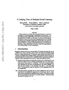
Figure 2. From left to right, sample from rectangles, rectanglesimage and convex.

4.2. Comparing with Deep Architectures

3

Code and data for all experiments in this paper are available at: https://github.com/michaelshiyu/kerNET.

We now evaluate MLKN on three classification benchmarks that have been specifically created with many factors of

Learning Multiple Levels of Representations with Kernel Machines Table 2. Test errors (%) and 95% confidence intervals (%). When two results have overlapping confidence intervals, they are considered equivalent. Best results are marked in bold.

MODEL

MLP-2 DBN-3 SAE-3 MLKN-2

RECTANGLES

RECTANGLES - IMAGE

7.16± 0.23 2.60± 0.14 2.41± 0.13 2.44± 0.14

33.20± 0.41 22.50± 0.37 24.05± 0.37 23.93± 0.37

CONVEX

32.25± 0.41 18.63± 0.34 18.41± 0.34 20.13± 0.35

variation to empirically show that deep architectures are favorable for these complex tasks (Larochelle et al., 2007). We use these benchmarks to show that MLKN, as a deep architecture itself, is competitive with other popular deep models including MultiLayer Perceptron (MLP), Deep Belief Network (DBN) and Stacked Autoencoder (SAE). The data sets consist of 28 × 28 grayscale images. The first data set, known as rectangles, has 1000 training images, 200 validation images and 50000 test images. The learning machine is required to tell if a rectangle contained in an image has a larger width or length. The location of the rectangle is random. The border of the rectangle has pixel value 255 and pixels in the rest of an image all have value 0. The second data set, rectangles-image, is essentially the same with rectangles except that the inside and outside of the ractangle are replaced by an image patch, respectively. rectanglesimage has 10000 training images, 2000 validation images and 50000 test images. The third data set, convex, consists of images in which there are white regions (pixel value 255) on black (pixel value 0) background. The learning machine needs to distinguish if the region is convex. This data set has 6000 training images, 2000 validation images and 50000 test images. Sample images from the three data sets are given in Figure 2. For actual training and testing, the pixel values are normalized to [0, 1]. For detailed descriptions for those data sets, see (Larochelle et al., 2007). The experimental settings are as follows, we use a two-layer MLKN (MLKN-2) with the first layer consisting of 15 kernel machines with the same Gaussian kernel and the second layer being a single kernel machine with another Gaussian kernel. The model is trained with the proposed greedy learning algorithm. For the kernel machine on the second layer, instead of as a SVM, it is trained with gradient descent and cross-entropy as cost function for a fair comparison with the other deep architectures. Hyperparameters including kernel widths, regularization coefficients and step size for gradient descent are selected using the validation set. The validation set is then used in final training only for early-stopping based on validation set classification error. We compare MLKN with a two-layer MLP (MLP-2), a three-layer DBN (DBN-3) and a three-layer SAE (SAE-3). MLP serves as a baseline for comparison. For those models,

layer sizes and hyperparameters are also selected using the validation set. During model selection, for MLP, the size of the hidden layer ranges from 25 to 700; for DBN-3 and SAE3, the sizes of the three layers vary in intervals [500, 3000], [500, 4000] and [1000, 6000], respectively. This means that the dimension of any of the representation spaces of any of these architectures is significantly larger than that of MLKN-2 (for MLKN-2, there is one representation space with dimension 15). Also note that although the number of parameters of a kernel machine scales linearly with the size of the training set, MLKN-2 actually has the second smallest number of parameters among all 4 models in all 3 data sets, both DBN-3 and SAE-3 have significantly more trainable parameters than MLP-2 and MLKN-2. Like in the training for MLKN-2, the validation set is also reserved for early-stopping in final training. SAE-3 and DBN-3 are pre-trained unsupervisedly before the supervised training phase, following the algorithms described in (Hinton et al., 2006; Bengio et al., 2007). More detailed settings for these models are reported in (Larochelle et al., 2007). From Table 2, we see that the performance of MLKN is on par with some of the most popular and most mature deep architectures even though both the hidden layer dimension and the number of parameters of the MLKN used to achieve those results are much smaller than that of any of the other models. In terms of the broadness of the function space induced by these deep architectures, there is no need to distinguish between any two of them since they are all dense subsets of a bigger function space of practical interest, such as CC (X). However, since the function space induced by a kernel machine is an inner product space, it is much more tractable to theoretical analysis thanks to many useful mathematical constructions such as orthogonality being defined in an inner product space. Hence we propose MLKN not to compete with or eliminate any existing deep architecture but in the hope that it can make possible interesting theoretical discoveries that unveil what makes deep architectures so powerful in the most challenging machine learning problems.

5. Conclusion We presented a deep architecture based on kernel machines. Compared to traditional kernel machines, our construction is capable of learning hierarchical, distributed representations. Moreover, it is more robust to the choice of kernel. Compared to other deep architectures, our model can be trained in a layer-wise fashion and has a more well-structured underlying function space, making it more tractable to theoretical analysis. We reported favorable results on multiple classification benchmarks.

Learning Multiple Levels of Representations with Kernel Machines

References Aronszajn, N. Theory of reproducing kernels. Transactions of the American mathematical society, 68(3):337–404, 1950.

Lanckriet, G. R., Cristianini, N., Bartlett, P., Ghaoui, L. E., and Jordan, M. I. Learning the kernel matrix with semidefinite programming. Journal of Machine learning research, 5(Jan):27–72, 2004.

Bach, F. R., Lanckriet, G. R., and Jordan, M. I. Multiple kernel learning, conic duality, and the smo algorithm. In Proceedings of the twenty-first international conference on Machine learning, pp. 6. ACM, 2004.

Larochelle, H., Erhan, D., Courville, A., Bergstra, J., and Bengio, Y. An empirical evaluation of deep architectures on problems with many factors of variation. In Proceedings of the 24th international conference on Machine learning, pp. 473–480. ACM, 2007.

Bengio, Y. Learning deep architectures for ai. Foundations R in Machine Learning, 2(1):1–127, 2009. and trends

LeCun, Y., Bengio, Y., and Hinton, G. Deep learning. Nature, 521(7553):436–444, 2015.

Bengio, Y., Lamblin, P., Popovici, D., and Larochelle, H. Greedy layer-wise training of deep networks. In Advances in neural information processing systems, pp. 153–160, 2007.

Mhaskar, H., Liao, Q., and Poggio, T. Learning functions: when is deep better than shallow. arXiv preprint arXiv:1603.00988, 2016.

Broomhead, D. S. and Lowe, D. Radial basis functions, multi-variable functional interpolation and adaptive networks. Technical report, Royal Signals and Radar Establishment Malvern (United Kingdom), 1988. Chen, S., Cowan, C. F., and Grant, P. M. Orthogonal least squares learning algorithm for radial basis function networks. IEEE Transactions on neural networks, 2(2): 302–309, 1991. Cho, Y. and Saul, L. K. Kernel methods for deep learning. In Advances in neural information processing systems, pp. 342–350, 2009. Cortes, C. and Vapnik, V. Support-vector networks. Machine learning, 20(3):273–297, 1995. Cristianini, N. and Shawe-Taylor, J. An introduction to support vector machines and other kernel-based learning methods. Cambridge university press, 2000. Cristianini, N., Shawe-Taylor, J., Elisseeff, A., and Kandola, J. S. On kernel-target alignment. In Advances in neural information processing systems, pp. 367–373, 2002. Gehler, P. and Nowozin, S. Infinite kernel learning. 2008. G¨onen, M. and Alpaydın, E. Multiple kernel learning algorithms. Journal of machine learning research, 12(Jul): 2211–2268, 2011.

Micchelli, C. A., Xu, Y., and Zhang, H. Universal kernels. Journal of Machine Learning Research, 7(Dec):2651– 2667, 2006. Nair, V. and Hinton, G. E. Rectified linear units improve restricted boltzmann machines. In Proceedings of the 27th international conference on machine learning (ICML-10), pp. 807–814, 2010. Park, J. and Sandberg, I. W. Universal approximation using radial-basis-function networks. Neural computation, 3 (2):246–257, 1991. Principe, J. C., Xu, D., and Fisher, J. Information theoretic learning. Unsupervised adaptive filtering, 1:265–319, 2000. Rahimi, A. and Recht, B. Random features for large-scale kernel machines. In Advances in neural information processing systems, pp. 1177–1184, 2008. Rumelhart, D. E., Hinton, G. E., and Williams, R. J. Learning representations by back-propagating errors. Nature, 323(6088):533–538, 1986. Sch¨olkopf, B. and Smola, A. J. Learning with kernels: support vector machines, regularization, optimization, and beyond. MIT press, 2001. Sch¨olkopf, B., Herbrich, R., and Smola, A. J. A generalized representer theorem. In Computational learning theory, pp. 416–426. Springer, 2001.

Hinton, G. E., Osindero, S., and Teh, Y. W. A fast learning algorithm for deep belief nets. Neural computation, 18 (7):1527–1554, 2006.

Varma, M. and Babu, B. R. More generality in efficient multiple kernel learning. In Proceedings of the 26th Annual International Conference on Machine Learning, pp. 1065–1072. ACM, 2009.

Kloft, M., Brefeld, U., Sonnenburg, S., and Zien, A. Lpnorm multiple kernel learning. Journal of Machine Learning Research, 12(Mar):953–997, 2011.

Williams, C. K. and Seeger, M. Using the nystr¨om method to speed up kernel machines. In Advances in neural information processing systems, pp. 682–688, 2001.

Learning Multiple Levels of Representations with Kernel Machines

Xu, Z., Jin, R., King, I., and Lyu, M. An extended level method for efficient multiple kernel learning. In Advances in neural information processing systems, pp. 1825–1832, 2009. Zhuang, J., Tsang, I. W., and Hoi, S. C. Two-layer multiple kernel learning. In Proceedings of the Fourteenth International Conference on Artificial Intelligence and Statistics, pp. 909–917, 2011.

Learning Multiple Levels of Representations with Kernel Machines

A. Proofs Proposition A.1. Given a random sample S ⊆ X belonging to an arbitrary number of classes, if k : X × X → R is a kernel that induces the ideal Gram matrix on S as defined in Section 2.3, then in the RKHS induced by k, denoted by H, the images of the random sample under the kernel mapping Φ( · ) has the following property: Φ(xi ) and Φ(xj ) are orthogonal if xi , xj ∈ S belong to different classes; Φ(xi ) = Φ(xj ) if xi , xj ∈ S belong to the same class. Proof. To see this, first note that k(xi , xj ) = hΦ(xi ), Φ(xj )iH = 0 if xi , xj are not in the same class implies that Φ(xi ), Φ(xj ) are orthogonal whenever xi , xj are from different classes. And since hΦ(xi ), Φ(xj )iH = 1 if xi , xj are in the same class, in particular, hΦ(xi ), Φ(xi )iH = 1 for all i, kΦ(xi )kH = 1 for all i, where, of course, we have used the norm induced by the inner product h · , · iH . Since k is unsigned when restricted to S × S, by Cauchy-Schwarz, for all xi , xj ∈ S, hΦ(xi ), Φ(xj )iH ≤ kΦ(xi )kH kΦ(xj )kH and the equality holds if and only if Φ(xi ) = CΦ(xj ) for some nonzero constant C. Using kΦ(xi )kH = 1 for all i, we further conclude that the equality holds if and only if C = 1. As a result, k(xi , xj ) = hΦ(xi ), Φ(xj )iH = 1 if xi , xj are from the same class implies Φ(xi ) = Φ(xj ) when xi , xj are in the same class. Proposition A.2. Given a random sample S ⊆ X belonging to an arbitrary number of classes, assume k : X × X → R is an unsigned kernel with the property k(x, x) = 1, ∀x ∈ X and the Gram matrix induced by k on S is the ideal Gram matrix as defined in Section 2.3. For any two classes from Φ(S), the margin with respect to the class of all linear functions in H is no smaller than that of Φ(T ), where Φ( · ) and H are the kernel mapping and the RKHS induced by k, respectively, and T is any other random sample from X.

all functions in F, denoted γ, is called the margin of S with respect to F. Now consider the kernel k in the assumption. Since k is unsigned, the inner product between Φ(xi ), Φ(xj ) is nonnegahΦ(x ), Φ(xj )iH tive for any xi , xj ∈ X, so is cos θi,j = kΦ(xi )ki H kΦ(x , j )kH where θi,j is the angle between Φ(xi ), and Φ(xj ). Hence the angle between any two vectors in H is less than or equal to π2 . Since kΦ(xi )kH = 1, ∀xi ∈ X, for any two classes in a given random sample, the margin with respect to the set of all linear functions in H is maximized when Φ(xi ), Φ(xj ) are orthogonal if xi , xj are not from the same class. By construction, S is such a random sample. For any other random sample T ⊆ X, since it is not guaranteed that k induces an ideal Gram matrix on T , the corresponding margin is no larger than that of Φ(S). Remark The condition on k can be relaxed to k(x, x) = C, ∀x ∈ X for some nonzero constant C since one can always scale the kernel with C1 . Proposition A.3. Given random sample S = {x1 , x2 , ..., xn } ⊆ Rd and kernels k 1 , k 2 , ..., k m : Rd × Rd → R, let representation-learning layers F 1 ( · ), F 2 ( · ), ..., F m ( · ) : Rd → Rd be defined similarly to how F 1 ( · ) is defined in Subsection 2.1. Assume the alignment for each one of these layers is calculated with the same kernel k. Then for layer i = 1, 2, ..., m, the alignment ˆ i ◦ F i−1 ◦ · · · ◦ F 1 (S), k, G? ). Suppose is denoted A(F each layer is trained greedily with gradient descent. When all layers have been fully trained, that is, gradient descent has converged to a local or global minimum according to some reasonable stopping criterion, for any i = 2, 3, ..., m and any j ≤ i, we have ˆ j ◦ F j−1 ◦ · · · ◦ F 1 (S), k, G? ) ≤ A(F ˆ i ◦ F i−1 ◦ · · · ◦ F 1 (S), k, G? ). A(F ˆ k, G? ) ≤ A(F ˆ 1 (S), k, G? ). For i = 1, we have A(S,

Proof. First, we include the definition of margin (Cristianini & Shawe-Taylor, 2000) for completeness. When using a class of real-valued functions F on H for classification by thresholding at 0 and let a random sample S ⊆ X with labels taking values from {−1, 1} be given, the margin of an example (xi , yi ) ∈ S × {−1, 1} with respect to a function f from the given function class is defined as γi = yi f (xi ). And the minimum of the margins of all examples in S is refered to as the margin of f with respect to S. When the function class consists only of linear functions and assuming an inner product h · , · i is defined for the space in which the functions in the class are linear, the margin of a function in it becomes γw,b = min(xi , yi )∈S (yi (hw, xi i + b)), where b ∈ R is the bias of the hyperplane. And interpretation for γw,b is geometric: it is the smallest (signed) distance between examples and the hyperplane. The maximum margin over

Proof. Fix an i, assume all layers up to but not including layer i have been fully trained with the layer-wise learning algorithm, i.e., all mappings in the compositon F i−1 ◦ · · · ◦ F 1 ( · ) have been determined by the learning algorithm and F i−1 ◦ · · · ◦ F 1 (S) is hence a fixed set of vectors in Rd . We first show that we can initialize F i ( · ) to the initial state F i∗ ( · ) such that F i∗ ◦ F i−1 ◦ · · · ◦ F 1 (S) = F i−1 ◦ · · · ◦ F 1 (S), that is, initialize the map F i ( · ) to be the identity map restricted to F i−1 ◦ · · · ◦ F 1 (S). Without loss of generality, assume i = 1, then it amounts to showing that a set of parameters on kernel machines in F 1 ( · ) can be found such that when these kernel machines are initialized with this certain set of parameters, F 1∗ (S) = S. For j = 1, 2, ..., d,P denote the j th kernel machine on the first layer as n fj ( · ) = i=1 αji k 1 (xi , · ).

Learning Multiple Levels of Representations with Kernel Machines

If k 1 is strictly PD, solving equation A> G = S for A, where A is a n × d matrix of parameters defined as [A]ij = αji , G is the n × n Gram matrix defined as [G]ij = k 1 (xi , xj ), S is a d × n matrix whose ith column is the ith data point xi = [xi1 , xi2 , ..., xid ]> for i = 1, 2, ..., n, it is straightforward that the set of parameters A is the set needed for initializing the first layer to the desired state. Moreover, A can always be solved analytically since k 1 being strictly PD suggests G is invertible.

with the same k. These two assumptions are made for the need of the preceding proof. In our experiments, on the other hand, we have never followed those restrictions. Besides, we always initialize each layer randomly. However, the conclusion in Proposition A.3 has always been true in practice. Hence, the assumptions needed for the above proof may be more than what is actually needed for the layer-wise learning algorithm to possess the desirable property described in Proposition A.3.

If it is numerically unstable to invert A or if k 1 is PD, one should resort to an iterative method to find the initial set of parameters for F 1 ( · ). It is guaranteed that the identity map restricted to S can be uniformly approximated by F 1 ( · ). To see this, first find the smallest subspace in Rd that includes the set S by taking the intersection of all subspaces that include S. This minimal subspace is closed and bounded by construction hence is also compact. Further, this subspace is a Banach space since Rd is. Consequently, since the identity map restricted to this subspace is bounded by construction, it is continuous and hence in CC (Rd ) if we declare that it is 0 off the minimal subspace. By the universality assumption of k 1 and the representer theorem, F 1 ( · ) approximates the identity map on S uniformly if it is the optimal solution to some empirical risk defined for S. With the existence of an arbitrarily close approximation established, in practice,P one can optimize F 1 ( · ) to minimize n the empirical risk i=1 (F 1 (xi ) − xi )2 with any convex optimization technique and it is guaranteed that the optimal solution, which is the identity map on S by construction, can be implemented by F 1 ( · ). The resulting state of F 1 ( · ) after this optimization can be used to initialize F 1 ( · ). Note that in this case, one needs to tolerate an approximation error due to limitations of any iterative method used to find the parameters.

Lemma A.4. Given a random sample S ⊆ Rd and kernels k 1 , k 2 : Rd × Rd → R, let F 1 ( · ) : Rd → Rd be defined as in Subsection 2.1. When approximating a solution function f ∈ CC (Rd ) for any given empirical risk minimization problem, the best approximation in the span of Φ2 (F 1 (S)) is no worse than that in Φ2 (S). Proof. Using what we have shown in Proposition A.3, we conclude that F 1 ( · ) can be initialized such that F 1 (S) = S. Then the conclusion follows from noting that the reasoning in Proposition A.3 can be easily generalized to any empirical risk apart from alignment. It also follows that although Lemma A.4 is only stated for the first layer, it is generalizable to any two adjacent layers in MLKN. Proposition A.5. Under the initialization condition in Proposition A.3, for layer i, assume k i+1 : Rm × Rm → R is a nontrivial function Pm of kx − ykp ,p1 ≤ p < ∞, where kx − ykp := t=1 [x]t − [y]t . Denote the states of the kernel machines on layer i after training i◦ as f1i◦ ( · ), f2i◦ ( · ), ..., fm ( · ). Then the probability of the i◦ (pointwise) equivalence f1i◦ = f2i◦ = · · · = fm being true is strictly smaller than 1.

Inductively, similar result can be proven for any layer and Proposition A.3 is hence proved.

Proof. That the optimization is nonconvex for layer i if k i+1 is nonlinear is straightforward. Denote the initial states of i f1i ( · ), f2i ( · ), ..., fm ( · ) under the initialization condition in i∗ Proposition A.3 as f1i∗ ( · ), f2i∗ ( · ), ..., fm ( · ), then it is also obvious that the probability of the (pointwise) equivalence i∗ f1i∗ = f2i∗ = · · · = fm being true is strictly smaller than 1. Since the optimization is based on gradiet descent, it is sufficient to prove that the derivative of the cost function with respect to a parameter on fsi ( · ) is not necessarily equal to the derivative of the cost function with respect to the corresponding parameter on fti ( · ) for s 6= t.

Remark Note that in the architecture and learning algorithm described in Section 2, the dimension of each layer can surely be chosen freely and alignment at each layer is calculated using the kernel from the next layer. However, in Proposition A.3 we have implicitly assumed that all layers up to layer n are of the same dimension. Also, we have assumed that alignments for those layers are all calculated

For simplicity, we consider Mean Square Error (MSE) instead of alignment to be the cost function for layer i, which is also a valid cost function to carry out the learning objective in Subsection 2.3. The proof for alignment follows the same strategy but the derivation is slightly more cumbersome. Without loss of generality, let i = 1. For a specific parameter αsv on the sth kernel machine fs1 ( · ) = Pn 1 g=1 αsg k (xg , · ), where s = 1, 2, ..., m, v = 1, 2, ..., n,

Now suppose the first layer has been trained with the greedy learning algorithm and gradient descent has successfully converged according to some reasonably given criterion. Denote the state of the first layer after training with F 1 ( · ), by nature of gradient, namely, it always points at the direction of maximum increase of the function, we then have ˆ k, G? ) = A(F ˆ 1∗ (S), k, G? ) ≤ A(F ˆ 1 (S), k, G? ), A(S,

Learning Multiple Levels of Representations with Kernel Machines

we have

setting within any representation-learning layer of MLKN in order to learn complicated representations.

∂M SE(G? , G2 ) ∂αsv n 2 X ? ∂ n12 [G ]i,j − [G2 ]i,j i,j=1

=

∂αsv n

=

Note that Proposition A.5 only characterizes a class of kernels that result in potentially different gradient for each kernel machine within a layer. There are surely more kernels with this desirable property than what we have described here. And it is easy enough to check for any specific kernel.

2 X

?

[G ]i,j

n2

i,j=1



=−

∂ [G? ]i,j − [G2 ]i,j − [G2 ]i,j ∂αsv 2

n ? 2 2 X [G ]i,j − [G ]i,j ∂[G2 ]i,j n2 i,j=1

[G? ]i,j − [G2 ]i,j

∂αsv

2   n ? 2 2 X ] − [G ] F 1 (xi ), F 1 (xj ) [G i,j i,j ∂k 2 =− 2 n [G? ]i,j − [G2 ]i,j ∂αsv i,j=1 p ∂ fs1 (xi ) − fs1 (xj ) =C ∂αsv p−1 ∂ fs1 (xi ) − fs1 (xj ) = Cp fs1 (xi ) − fs1 (xj ) ∂αsv p  1 1  fs (xi ) − fs (xj ) 1 1 k (x , x ) − k (x , x ) , = Cp 1 v i v j fs (xi ) − fs1 (xj ) (1) where C is some term that depends on the specific function form of k 2 and is the same for all s. From Equation 1, we can see that the gradient of each kernel machine at each iteration depends on its own past state, and since the initial states of the kernel machines are different and the performance surface of each kernel machine has multiple local minima, the probability that all kernel machines within one layer converge to the same local minimum is strictly less than 1, which proves Proposition A.5. Remark For neural networks, even with uniformity within layers and full connectivity between layers, derivatives for parameters in each unit within any layer are not necessarily identical across units, as suggested by backpropagation, in particular, chain rule. This observation makes neural networks particularly interesting and efficient as representation learning models since diversity in solution functions is possible even when all units on a layer are identical in construction. On the other hand, Proposition A.5 has shown that under mild conditions on k i+1 , kernel machines on layer i will very likely have distinct gradient information and hence learn different solution functions, enriching the resulting internal representation at that layer. This observation justifies having multiple kernel machines with the same

Proposition A.6. A two-layer MLMKL is a special case of a two-layer that is, given sets of functions n PMLKN, P Pd N d MLMKL := 1 1 F i=1 γi k( t=1 µt ft (xi ), t=1 µt ft ( · )) : o N ∈ N, γi ∈ R, µt ∈ R+ and F MLKN := nP o N 1 1 β k(F (x ), F ( · )) : N ∈ N, β ∈ R , we have i i i=1 i F MLMKL ( F MLKN . The strict set inclusion holds true regardless of whether kernels used by MLMKL and MKLN are the same. Proof. Without loss of generality, let d = 2. Since all kernels in the constructions are universal by assumption, it is sufficient to prove following: define a linear functional T : A ⊆ R2 → R as T (x, y) = ax + by, where A is a compact subspace in R2 , a, b ∈ R are arbitrary. Consider its adjoint ∗ T ∗ : CC (R) → CC (R2 ), (Ta,b f )(x, y) = f (T (x, y)) = ∗ (CC (R)) ( CC (R2 ). f (ax + by). Then we have ∪a,b∈R Ta,b The set inclusion is automatic since the composition of continuous functions is continuous, we prove the inequality by contradiction. Suppose for every g ∈ CC (R2 ), there exists h ∈ CC (R) and a, b ∈ R such that for any r ∈ R, the preimages characterized by g(x, y) = r and by h(ax + by) = r are identical. Pick g(x, y) = x2 + y 2 , suppose h ∈ CC (R) and a, b ∈ R is a valid choice. g(x, y) = x2 + y 2 = r parameterizes a circle centered around the origin for r > 0. Fix a r > 0, find the set Z = {z : h(z) = r} for the chosen h, h(ax + by) = r = h(z) parameterizes the line ax + by = z, which suggests the set {(x, y) : (x, y) ∈ R2 , ax + by = z, z ∈ Z} specifies a union of lines, which cannot be identical to the circle {(x, y) : (x, y) ∈ R2 , x2 + y 2 = r}, hence there does not exist h ∈ CC (R) and a, b ∈ R such that g(x, y) = x2 + y 2 and h(ax + by) are equal as functions. Hence ∗ ∪a,b∈R Ta,b (CC (R)) ( CC (R2 ). Note that in the above proof, we have not taken into account the constraint that the kernel combination coefficients µt being positive in MLMKL, which will make the set F MLMKL even smaller.