Learning Summary Statistic for Approximate Bayesian Computation ...

Learning Summary Statistic for Approximate Bayesian Computation via Deep Neural Network

arXiv:1510.02175v1 [stat.ME] 8 Oct 2015

Bai Jiang, Tung-yu Wu, Charles Zheng and Wing H. Wong Stanford University

Abstract: Approximate Bayesian Computation (ABC) methods are used to approximate posterior distributions in models with unknown or computationally intractable likelihoods. Both the accuracy and computational efficiency of ABC depend on the choice of summary statistic, but outside of special cases where the optimal summary statistics are known, it is unclear which guiding principles can be used to construct effective summary statistics. In this paper we explore the possibility of automating the process of constructing summary statistics by training deep neural networks to predict the parameters from artificially generated data: the resulting summary statistics are approximately posterior means of the parameters. With minimal model-specific tuning, our method constructs summary statistics for the Ising model and the moving-average model, which match or exceed theoreticallymotivated summary statistics in terms of the accuracies of the resulting posteriors. Key words and phrases: Approximate Bayesian Computation, Summary Statistic, Deep Learning

1. Introduction Bayesian inference is traditionally centered around the ability to compute or sample from the posterior distribution of the parameters, having conditioned on the observed data. Suppose data X is generated from a model M with parameter

θ, the prior of which is denoted by π(θ). If the closed form of the likelihood function l(θ) = p(X|θ) is available, the posterior distribution of θ given observed data xobs can be computed via Bayes’ rule π(θ|xobs ) =

π(θ)p(xobs |θ) . p(xobs )

2

Bai Jiang, Tung-yu Wu, Charles Zheng and Wing Wong

Alternatively, if the likelihood function can only be computed conditionally or up to a normalizing constant, one can still draw samples from the posterior by using stochastic simulation techniques such as Markov Chain Monte Carlo (MCMC) and rejection sampling (Asmussen and Glynn (2007)). However, in many applications, the likelihood function l(θ) = p(X|θ) cannot be explicitly obtained, or is intractable to compute; this precludes the possibility of direct computation or MCMC sampling. In these cases, approximate inference can still be performed so long as 1) it is possible to draw θ from the prior π(θ), and 2) it is possible to simulate X from the model M given θ, using the meth-

ods of Approximate Bayesian Computation (ABC) (See e.g. Beaumont, Zhang and Balding (2002); Lopes and Beaumont (2010); Beaumont (2010); Csilléry,

Blum, Gaggiotti and Fran¸cois (2010); Marin, Pudlo, Robert and Ryder (2012); Toni, Welch, Strelkowa, Ipsen and Stumpf (2009); Sunn˚ aker, Busetto, Numminen, Corander, Foll and Dessimoz (2013)). While many variations of the core approach exist, the fundamental idea underlying ABC is quite simple: that one can use rejection sampling to obtain draws from the posterior distribution π(θ|xobs ) without computing any likelihoods. We draw parameter-data pairs (θ0 , X 0 ) from the prior π(θ) and the model M, and

accept only the θ0 such that X 0 = xobs , which occurs with conditional probability

p(xobs |θ0 ) for any θ0 . Algorithm 1 describes the ABC method for discrete data (Tavaré, Balding, Griffiths and Donnelly (1997)), which yields an i.i.d. sample {θ(i) , 1 ≤ i ≤ n} of the exact posterior distribution π(θ|X = xobs ). Algorithm 1 ABC rejection sampling 1 for i = 1, ..., n do repeat Propose θ0 ∼ π(θ) Draw X 0 ∼ M given θ0 until X 0 = xobs (acceptance criterion) Accept θ0 and let θ(i) = θ0 end for

The success of Algorithm 1 depends on acceptance rate of proposed parameter θ0 , i.e. the probability of the event X 0 = xobs given θ. For continuous xobs and X 0 , the event X 0 = xobs happens with probability 0, and hence Algorithm

Learning Summary Statistic for ABC via DNN

3

1 is unable to produce any draws. As a remedy, one can relax the acceptance criterion X 0 = xobs to be kX 0 − xobs k < , where k · k is a norm and is the

tolerance threshold. The choice of is crucial for balancing efficiency and ap-

proximation error, since with smaller the approximation error decreases while the acceptance probability also decreases. However, when the observation vectors are high-dimensional, the inefficiency of rejection sampling in high dimensions results in either extreme inaccuracy, or accuracy at the expense of an extremely time-consuming procedure. To circumvent the problem, one can introduce low-dimensional summary statistic S and further relax the acceptance criterion to be kS(X 0 ) − S(xobs )k < . The use of summary statistics results in Algorithm 2, which was first proposed as the

extension of Algorithm 1 in population genetics application (Fu and Li (1997); Weiss and von Haeseler (1998); Pritchard, Seielstad, Perez-Lezaun and Feldman (1999)). Algorithm 2 ABC rejection sampling 2 for i = 1, ..., n do repeat Propose θ0 ∼ π Draw X 0 ∼ M with θ0 until kS(X 0 ) − S(xobs )k < (relaxed acceptance criterion) Accept θ0 and let θ(i) = θ0 end for

Instead of the exact posterior distribution, the resulting sample {θ(i) , 1 ≤

i ≤ n} obtained by Algorithm 2 follows an approximate posterior distribution π(θ|kS(X 0 ) − S(xobs )k < ) ≈ π(θ|S(X) = S(xobs )) ≈ π(θ|X = xobs ).

(1.1) (1.2)

The choice of the summary statistic is crucial for the approximation quality of ABC posterior distribution. A good summary statistic should offer a good tradeoff between two approximation errors (Blum, Nunes, Prangle, Sisson and others (2013)). The approximation error (1.1) is introduced when one replaces “equal to” with “similar” in the first relaxation of the acceptance criterion. Under appropriate regularity conditions, it vanishes as → 0. The approximation error

4


(1.2) is introduced when one compares summary statistics S(X) and S(xobs ) rather than the original data X and xobs . In essence, this is just the information loss of mapping high-dimensional X to low-dimensional S(X). A summary statistic S of higher dimension is in general more informative, hence reduces the approximation error (1.2). But at the same time, increasing the dimension of the summary statistic slows down the rate that the approximation error (1.1) vanishes in the limit of → 0. Ideally, we seek a statistic which is simultaneously

low-dimensional and informative.

A sufficient statistic is an attractive option, since sufficiency, by definition, implies that the approximation error (1.2) is zero (Lehmann and Casella (1998)). However, the sufficient statistic has generally the same dimensionality as the sample size, except in special cases such as exponential families. And even when a low-dimensional sufficient statistic exists, it may be intractable to compute. The main task of this article is to construct low-dimensional and informative summary statistics for ABC methods. Since our goal is to compare methods of constructing sufficient statistics (rather than present a complete methodology for ABC), the relatively simple Algorithm 2 suffices. In future work, we plan to use our approach for constructing summary statistics alongside more sophisticated variants of ABC methods, such as those which combine ABC with Markov chain Monte Carlo or sequential techniques (Marjoram, Molitor, Plagnol and Tavaré (2003); Sisson, Fan and Tanaka (2007)). Hereafter all ABC procedures we mentioned in this paper use Algorithm 2. Existing methods for constructing summary statistics can be roughly classified into two classes (Blum, Nunes, Prangle, Sisson and others (2013)), both of which require a set of candidate summary statistics. The first class consists of approaches for best subset selection. Subsets of the candidate set of summary statistics are evaluated according to various information-based criteria, e.g. measure of sufficiency (Joyce and Marjoram (2008)), entropy (Nunes and Balding (2010)), AIC (Blum, Nunes, Prangle, Sisson and others (2013)) and BIC (Blum, Nunes, Prangle, Sisson and others (2013)), and the “best” subset is chosen to be the summary statistic. The second class is projection approach, which constructs summary statistics by linear or non-linear regression on the candidate set (Boulesteix and Strimmer (2007); Wegmann, Leuenberger and Excoffier


5

(2009); Blum and Fran¸cois (2010); Fearnhead and Prangle (2012)). Many of these methods require both expert knowledge and candidate summary statistics. An exception is Fearnhead and Prangle (2012)’s semi-automatic method, in which the authors take powers of individual data points as the initial candidate set and use linear regression to construct summary statistics. Here we use deep neural networks (DNN) to automatically learn summary statistics for high-dimensional X. Blum and Fran¸cois (2010) has also considered the use of artificial neural networks for nonlinear projection; however, we are the first to consider the use of multilayer neural networks. The additional representational power offered by DNNs (compared to single-layer networks or other nonlinear function classes) enables our approach to be effective even without the need to specify an initial set of candidate statistics. In all of our experiments, we simply use the original data points as the input. Since we rely on the DNNs to automatically learn the appropriate nonlinear transformations which are necessary to construct useful summaries from the raw data, there is also no need to consider choosing a basis expansion of the original data points as in Fearnhead and Prangle (2012)’s semi-automatic method. Thus our choice of using DNNs allows to achieve a much higher degree of automation in constructing summary statistics than previous approaches. Our procedure for constructing summary statistics is as follows: (i) Generate a training set {θ(i) , X (i) } from prior π(θ) and the model M, (ii) Train a DNN, with X (i) as input and θ(i) as target, ˆ (iii) Use the estimator θ(X) as summary statistics in ABC procedure. The DNNs in our approach compose non-linear transformations of data in the hidden layers, and fit linear regressions in the output layer with neurons in the top hidden layer as explanatory variables. The idea is inspired by the notable successes of deep learning approach in several areas of machine learning, especially computer vision and natural language processing (Hinton and Salakhutdinov (2006); Hinton, Osindero and Teh (2006); Bengio, Courville and Vincent (2013); Schmidhuber (2015)). More and more practical and theoretical results show that deep architectures composed of simple learning modules in multiple layers can model high-level abstraction in

6


high-dimensional data. Thus it is expected that DNNs can effectively learn a ˆ good approximation to the posterior mean θ(X) ≈ Eπ (θ|X) under squared error loss, given a sufficiently large training set.

Our motivation for using an approximation of Eπ (θ|X) as a summary statistic for ABC is inspired by results of Fearnhead and Prangle (2012) which demonstrate that the use of the posterior mean Eπ (θ|X) optimizes certain criteria for first-order optimality. In a theoretical section, we extend their results and provide a simple proof in Theorem 1 based on conditioning, which is different to Fearnhead and Prangle (2012)’s proof via density-based calculation. In two simulated experiments, we construct summary statistics for Ising model and movingaverage model of order 2. Ising model has sufficient statistic, which is the ideal summary statistic but a highly non-linear function in high-dimensional space. It’s a challenging task to construct a summary statistic akin to such a sufficient statistic due to high non-linearity and high-dimensionality. However, we see in our experiments that the DNN-based summary statistic approximates an increasing function of the sufficient statistic. In contrast, the semi-automatic summary statistic is unable to capture information about interactions, and hence fails to approximate the sufficient statistic. For moving-average model of order 2, the DNN-based summary statistic outperforms the auto-covariance statistic, and the semi-automatic construction. It is noteworthy that an automatically constructed summary statistic can outperform auto-covariance in MA(2) model, since the auto-covariance can be transformed to yield a consistent estimate of the parameters, and was widely used in the literature. The rest of the article is organized as follows. In Section 2, we show how to construct summary statistics using deep neural networks. In Sections 3 and 4, we report the simulation studies on the Ising model and the moving average model, respectively. We describe in the supplementary materials the implementation details of training deep neural networks and other theoretical result, namely, how consistency can be obtained by using the posterior mean of a basis of functions of the parameters. 2. Methods Throughout the paper, we denote by M the model, X ∈ Rp the data, and

θ ∈ Rq the parameter. We assume it is possible to obtain a large number of


7

independent draws X ∼ p(·|θ). Denote by xobs the observed data, π the prior

of θ, S the summary statistic, k · k the norm to measure S(X) − S(xobs ), and

the tolerance threshold. Let πABC (θ) = π(θ|kS(X) − S(xobs )k < ) denote the

approximate posterior distribution obtained by Algorithm 2.

The main problem we address is how to construct a low-dimensional and informative summary statistic S for high dimensional X, which will enable accu rate approximation of πABC . We are interested mainly in the regime where ABC

is most effective: settings when the dimension of X is high (e.g. p = 100) and the dimension of θ is low (e.g. q = 1, 2). Given a prior π for θ, our approach is to (1) Generate a data set Dπ = θ(i)

from π and drawing

X (i)

(θ(i) , X (i) ), 1 ≤ i ≤ N from M with

by repeatedly drawing

θ(i) .

(2) Use Dπ to train a DNN with {X (i) , 1 ≤ i ≤ N } as input and {θ(i) , 1 ≤ i ≤ N } as target,

ˆ (3) Run ABC Algorithm 2 with prior π and the DNN estimator θ(X) as summary statistic. Our motivation for training a DNN to construct a summary statistic is that ˆ the resulting statistic should approximate the posterior mean S(X) = θ(X) ≈

Eπ (θ|X).

2.1. Posterior Means as Summary Statistics The main advantage of using the posterior mean Eπ (θ|X) as a summary statistic is that the ABC posterior distribution πABC (θ) will then have the same

mean as exact posterior distribution in the limit of → 0. That is to say, Eπ (θ|X) does not lose any first-order information when summarizing X. As Fearnhead

and Prangle (2012) discussed, using the posterior mean of the parameter itself as the summary statistic maximizes point-estimation accuracy under squarederror loss. We here provide a simple derivation for this extension in Theorem 1 based on conditioning, which is different to Fearnhead and Prangle (2012)’s proof via density-based calculation. We also provide in supplementary material an extension of Theorem 1 and show the convergence of the posterior expectation of b(θ) under the posterior obtained by ABC using Sb (X) = Eπ [b(θ)|X] as the

8


summary statistic. Such an extension further establishes a global approximation result of posterior distribution. Theorem 1. Assume Eπ |θ| < ∞, then statistic S(x) = Eπ (θ|X = x) is well defined. ABC procedure with observed data xobs , summary statistics S, norm

k · k and tolerance threshold produces a posterior distribution πABC . Then we

have

kEπABC θ − S(xobs )k < ,

and lim EπABC θ = Eπ (θ|X = xobs ).

→0

Proof. First, we show S(X) = Eπ (θ|X) is a version of conditional expectation of θ given S(X), i.e. S(X) = Eπ (θ|S(X)). Denote by σ(X), σ(S(X)) the σalgebras of X and S(X), respectively. Clearly S(X) = Eπ (θ|X) is measurable with respect to σ(S(X)). For any event A ∈ σ(S(X)), Eπ [S(X)IA ] = Eπ [Eπ (θ|X) IA ]

(by definition of S)

= Eπ {Eπ [Eπ (θ|X) IA |S(X)]}

(by tower property)

= Eπ {Eπ [Eπ (θ|X) |S(X)] IA }

(since A ∈ σ(S(X)))

= Eπ {Eπ (θ|S(X))IA } (by tower property and σ(S(X)) ⊆ σ(X)) Next, write EπABC b(θ) = Eπ [b(θ)|kSb (X) − Sb (xobs )k < ]

= Eπ [Eπ [b(θ)|Sb (X)]|kSb (X) − Sb (xobs )k < ] = Eπ [Sb (X)|kSb (X) − Sb (xobs )k < ] which, due to Jensen’s inequality, implies that kEπABC b(θ) − Sb (xobs )k = kEπ [Sb (X)|kSb (X) − Sb (xobs )k < ] − Sb (xobs )k

≤ Eπ [ kSb (X) − Sb (xobs )k| kSb (X) − Sb (xobs )k < ] 0 characterizes the extent of interaction.


13

Given θ, the probability mass function of Ising model on m × m lattice is P exp θ j∼k Xj Xk p(X|θ) = Zθ where Xj ∈ {−1, +1}, j ∼ k means Xj and Xk are neighbors, and the normalizing constant

 Zθ =

X

exp θ

x0 ∈{−1,+1}m×m

 X

x0j x0k  .

j∼k

Since the normalizing constant requires an exponential-time computation, the probability mass function p(x|θ) is intractable except in small cases. The Ising model is a natural exponential family with minimal sufficient statistics X S ∗ (X) = Xj Xk , j∼k

which is a highly non-linear function in high-dimensional space {−1, +1}10×10 .

Despite of the unavailability of probability mass function, data X can be

still simulated given θ using Monte Carlo methods such as Metropolis algorithm (Asmussen and Glynn (2007)). The Ising model on a square lattice undergoes a phase transition as θ increases. When θ is small, the spins are disordered. When θ is large enough, the spins tend to have the same sign due to the strong neighbour-to-neighbour interactions (Onsager (1944)). The phase transition of Ising model on infinite lattice has a critical point θc = 0.4406. Ising model on finite lattice is slightly different: its phase transition smoothly occurs around that critical point (Fearnhead and Prangle (2012)). So we consider Ising model on 10 × 10 lattice and choose the prior π ∼ Exp(0.4406) for θ.

The DNN-based summary statistic S(X) approximates the posterior mean,

which in turn is an increasing function of the sufficient statistic S ∗ (X), since the Ising model is an exponential family. Hence, for the evaluation purpose, we compare our DNN-based summary statistic S(X) to the minimal sufficient statistic S ∗ (X), and further compare the two resulting ABC posterior distributions. It’s a challenging task to constructing such a summary statistic S(X) P due to the high non-linearity of the sufficient statistic S ∗ (X) = j∼k Xj Xk in the high-dimensional space {−1, +1}10×10 where X lies in. Given the prior

π ∼ Exp(0.4406) for θ, we generate a training set by Metropolis algorithm, and

14


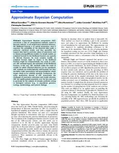
train a DNN to learn summary statistic S. We then compare S(X) to the known sufficient statistic S ∗ (X). Figure 4 outlines this experimental scheme.

{S ∗ (X (i) )}

known sufficient statsitics

compare

{θ(i) }

Ising model

{X (i) }

Deep Neural Network

{S(X (i) )}

supervised learning

Figure 4: Experimental design on Ising model

3.2. Results Given the prior π ∼ Exp(0.4406), we generate a training set of size 106 and a

testing set of size 105 from the Ising model on 10 × 10 lattice. As discussed in

Section 3.1, large θ tends to produce X which consists entirely of either +1 or −1. Consistent with this, 22.8% of generated test instances have spins with the

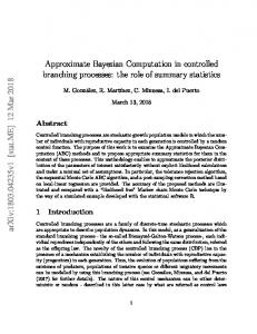
same sign, which results in sufficient statistic S ∗ = 200, and 4.7% of the test instances have all but one spins with the same sign, resulting in S ∗ = 192. A three-layer DNN with n(1) = 500, n(2) = 200, and n(3) = 100 in each hidden layer is trained to predict θ from x; we define the summary statistic S(x) as the output of the DNN. Figure 5a displays a scatterplot which compares the DNN-based statistic S and sufficient statistic S ∗ . Each point in the scatterplot represents to (S ∗ (x), S(x)) for a single instance x in the testing set. A large number of the instances are concentrated at S ∗ = 200 and S ∗ = 192, which appear as points in the top-right corner of the scatterplot. These two cases are relatively uninteresting, so in Figure 5b we display a heatmap of (S(x), S ∗ (x)) excluding the instances with S ∗ = 192, 200. It shows that the DNN-based summary statistic


15

approximates a strictly increasing function of sufficient statistic.

(a) Scatterplot of 105 test instances. Each point in the scatterplot represents to (S ∗ (x), S(x)) for a single test instance x.

(b) Heatmap excluding instances with sufficient statistic S ∗ = 192, 200

Figure 5: DNN-based summary statistic S v.s. sufficient statistic S ∗ on the test dataset.

16


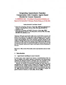
(a) True θ = 0.2

(b) True θ = 0.4

(c) True θ = 0.6

(d) True θ = 0.8

Figure 6: ABC posterior distributions for xobs generated with true θ = 0.2, 0.4, 0.6, 0.8.

Next, two ABC posterior distributions are obtained with S ∗ and S as summary statistic, respectively. For the sufficient statistic S ∗ , we set the tolerance level = 0 so that the ABC posterior sample follows the exact posterior distribution π(θ|X = xobs ). For the DNN-based summary statistic S, we set the tolerance threshold small enough so that 0.1% of 106 proposed θ0 s are accepted. We repeat the comparison for 4 different observed data xobs , which are generated from θ = 0.2, 0.4, 0.6, 0.8, respectively; in each case, we compare the posterior


17

obtained from S ∗ with the posterior obtained from S in Figure 6. It is also worth highlighting the case with true θ = 0.8 in Figure 6d. Since with high probability the spins Xi have the same sign when θ is large, it becomes difficult to distinguish different values of θ above the critical point θc based on the data xobs . Hence we should expect the posterior be small below θc and have a similar shape to the prior distribution above θc . Both of the ABC posteriors demonstrate this property. 4. Example: Moving-average Model 4.1. Model Description and Experiment Design The moving-average model is widely used in time series analysis. Each value in the time series is described by a linear combination of current and previous unobserved white noise error terms. Let X1 , . . . , Xp denote the observations in time series. Then the moving-average model of order q, denoted by MA(q) is given by Xj = Zj + θ1 Zj−1 + θ2 Zj−2 + ... + θq Zj−q ,

j = 1, ..., p

where Zj are unobserved white noise error terms. In our experiments, we let i.i.d.

Zj ∼ N (0, 1) in order to enable exact calculation of the posterior distribution π(θ|xobs ), so that we can evaluate the accuracy of the ABC posterior distribution.

In the case that Zj ’s are non-Gaussian (e.g. Student’s t-distribution), the exact posterior distribution π(θ|xobs ) becomes intractable to compute, but ABC is still applicable. Approximate Bayesian Computation has been applied to study the posterior distribution of MA(2) model using the auto-covariance as the summary statistic Marin, Pudlo, Robert and Ryder (2012). The auto-covariance is a natural choice for the summary statistic in the MA(2) model because it converges to a one-toone function of underlying parameter θ = (θ1 , θ2 ) in probability as p → ∞, by the weak law of large number

p−1

AC1 =

1 X P Xj Xj+1 → E(X1 X2 ) = θ1 + θ1 θ2 p−1 j=1

p−2

AC2 =

1 X P Xj Xj+2 → E(X1 X3 ) = θ2 . p−2 j=1

18


Since the MA(2) model is identifiable over the triangular region θ1 ∈ [−2, 2],

θ2 ∈ [−1, 1],

θ2 ± θ1 ≥ −1,

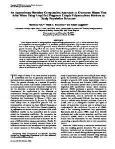
we consider a uniform prior π over this region, and proceed to construct a summary statistic similarly to the previous example. As before, we use the prior π to generate a training set and train a three-layer DNN to predict θ based on X. The two-dimensional estimator (S1 , S2 ) implicitly defined by DNN is taken as the summary statistic. We perform a number of experiments to compare the auto-covariance, the DNN-based summary statistic and semi-automatic summary statistic. In each experiment, we generate some true parameter θ from the prior, and draw the observed data xobs . The exact posterior distribution given xobs is numerically computed. Then we compute ABC posterior distributions using the auto-covariance statistic (AC1 , AC2 ), the DNN-based summary statistics (S1 , S2 ), and the semiautomatic summary statistic, respectively. The three resulting approximate posterior distributions are compared to the exact posterior distribution and evaluated in terms of the accuracies of posterior mean of θ, posterior marginal variances of θ1 , θ2 , and the posterior correlation between (θ1 , θ2 ). 4.2. Results Given the prior π, we generate a training set of size 106 and a testing set of size 105 from the MA(2) model, where each instance is a time series of length p = 100. Then a three-layer DNN with n(1) = 500, n(2) = 200, and n(3) = 100 is trained to predict θ from x. The summary statistic S(x) is defined as the output of the DNN. As shown in Figure 7, the DNN predicts θ1 , θ2 in the test set with mean squared errors (MSEs) of 0.021 and 0.024, respectively. In comparison, the semi-automatic method achieves MSEs of 0.678 and 0.189. For observed data xobs which is generated by true parameter θ drawn from π, we run ABC procedures with three different choices of summary statistic: the DNN-based summary statistic, the auto-covariance, and also the semi-automatic summary statistic. The tolerance threshold is set to accept 0.1% of 105 proposed data points in ABC procedures. Figure 8 compares the true posterior with the posterior draws obtained by ABC, for a particular xobs with θ = (0.6, 0.2). Using the DNN-based summary statistic results in a more accurate ABC posterior distribution than either the ABC posterior distribution obtained by


19

Figure 7: DNN predicting the parameters of MA(2) model for 105 test instances

using the auto-covariance statistic or the semi-automatic construction. One of the important features of the DNN-based summary statistic is its resulting ABC posterior correctly captures the correlation between θ1 and θ2 , while the autocovariance statistic and the semi-automatic statistic appears to be insensitive to

20


Figure 8: ABC posterior distributions (top: DNN-based summary statistics, middle: auto-covariance, bottom: semi-automatic construction) for observed data xobs generated with θ = (0.6, 0.2), compared to the exact posterior distribution contours.

this information (Table 1). We further repeated the comparison for 100 different xobs . As Table 2 shows, the ABC procedure with the DNN-based statistic better approximates the pos-


21

Table 1: Mean and covariance of exact/ABC posterior distributions for observed data xobs generated with θ = (0.6, 0.2) Posterior mean(θ1 ) mean(θ2 ) std(θ1 ) std(θ2 ) cor(θ1 , θ2 )

Exact 0.6243 0.3190 0.0910 0.1091 0.3664

ABC (DNN) 0.6567 0.2810 0.1174 0.1504 0.4110

ABC (auto-cov) 0.6760 0.5113 0.1386 0.2230 0.0471

ABC (semi-auto) -0.0030 0.2142 0.5540 0.4169 0.0205

terior moments than the ABC posteriors using the auto-covariance statistic and semi-automatic construction. Table 2: Mean squared error between mean and covariance of exact/ABC posterior distributions over 100 datasets

MSE for mean(θ1 ) MSE for mean(θ2 ) MSE for std(θ1 ) MSE for std(θ2 ) MSE for cor(θ1 , θ2 )

ABC (DNN) 0.0100 0.0119 0.0040 0.0042 0.0728

ABC (auto-cov) 0.0111 0.0184 0.0041 0.0065 0.1886

ABC (semi-auto) 0.5277 0.1466 0.4603 0.1002 0.2976

5. Discussion The problem that we address in this article is how to automatically construct lowdimensional and informative summary statistics for ABC methods, with minimal need for expert knowledge. We base our approach on theoretical results on the desirable properties of the posterior mean as a summary statistic for ABC. However, since the posterior mean is generally intractable, we take advantage of the representational power of DNNs to construct an approximation of the posterior mean as a summary statistic. In contrast to many existing methods that select or construct summary statistics from ad-hoc candidate summary statistics, our approach automatically searches through a rich class of nonlinear transformations of the input data to yield an appropriate summary statistic.

22

FIRSTNAME1 LASTNAME1 AND FIRSTNAME2 LASTNAME2

Although we can only heuristically justify our choice of DNNs to construct the approximation (due to a lack of rigorous theory on the approximation properties of DNNs), we obtain promising empirical results. In two examples, the Ising model and the moving-average model, we find that the the DNN-based statistics are good approximations of the posterior means, and further result in high-quality approximations to the true posterior distribution.

Supplementary Materials We first present in supplementary material an extension of Theorem 1 and show the convergence of the posterior expectation of b(θ) under the posterior obtained by ABC using Sb (X) = Eπ [b(θ)|X] as the summary statistic. Such an extension further establishes a global approximation result of posterior distribution as Theorem 2. Implementation details of backpropagation and stochastic gradient descent algorithms when training deep neural network are provided. The derivatives of squared error loss function with respect to network parameters are computed. They are used by stochastic gradient descent algorithms to train deep neural networks.

Acknowledgements The authors gratefully acknowledge National Science Foundation grants DMS1407557 and DMS1330132.

References Asmussen, S., and Glynn, P. W. (2007). Stochastic simulation: Algorithms and analysis (Vol. 57). Springer Science & Business Media. Beaumont, M. A., Zhang, W., and Balding, D. J. (2002). Approximate Bayesian computation in population genetics. Genetics, 162(4), 2025-2035. Lopes, J. S. and Beaumont, M. A. (2010). ABC: a useful Bayesian tool for the analysis of population data. Infection, Genetics and Evolution, 10(6), 825-832. Beaumont, M. A. (2010). Approximate Bayesian computation in evolution and ecology. Annual review of ecology, evolution, and systematics, 41, 379-406. Csilléry, K., Blum, M. G., Gaggiotti, O. E. and Fran¸cois, O. (2010). Approximate Bayesian computation (ABC) in practice. Trends in ecology & evolution, 25(7), 410-418.

REFERENCES23 Marin, J. M., Pudlo, P., Robert, C. P. and Ryder, R. J. (2012). Approximate Bayesian computational methods. Statistics and Computing, 22(6), 1167-1180. Toni, T., Welch, D., Strelkowa, N., Ipsen, A. and Stumpf, M. P. (2009). Approximate Bayesian computation scheme for parameter inference and model selection in dynamical systems. Journal of the Royal Society Interface, 6(31), 187-202. Sunn˚ aker, M., Busetto, A. G., Numminen, E., Corander, J., Foll, M. and Dessimoz, C. (2013). Approximate Bayesian computation. PLoS Comput. Biol., 9(1), e1002803. Tavaré, S., Balding, D. J., Griffiths, R. C. and Donnelly, P. (1997). Inferring coalescence times from DNA sequence data. Genetics, 145(2), 505-518. Fu, Y. X. and Li, W. H. (1997). Estimating the age of the common ancestor of a sample of DNA sequences. Molecular biology and evolution, 14(2), 195-199. Weiss, G. and von Haeseler, A. (1998). Inference of population history using a likelihood approach. Genetics, 149(3), 1539-1546. Pritchard, J. K., Seielstad, M. T., Perez-Lezaun, A., and Feldman, M. W. (1999). Population growth of human Y chromosomes: a study of Y chromosome microsatellites. Molecular biology and evolution, 16(12), 1791-1798. Blum, M. G., Nunes, M. A., Prangle, D., Sisson, S. A. and others (2013). A comparative review of dimension reduction methods in approximate Bayesian computation. Statistical Science, 28(2), 189-208. Lehmann, E. L. and Casella, G. (1998). Theory of point estimation (Vol. 31). Springer Science & Business Media. Marjoram, P., Molitor, J., Plagnol, V., and Tavaré, S. (2003). Markov chain Monte Carlo without likelihoods. Proceedings of the National Academy of Sciences, 100(26), 15324-15328. Sisson, S. A., Fan, Y. and Tanaka, M. M. (2007). Sequential monte carlo without likelihoods. Proceedings of the National Academy of Sciences, 104(6), 1760-1765. Joyce, P. and Marjoram, P. (2008). Approximately sufficient statistics and Bayesian computation. Statistical applications in genetics and molecular biology, 7(1). Nunes, M. A. and Balding, D. J. (2010). On optimal selection of summary statistics for approximate Bayesian computation. Statistical applications in genetics and molecular biology, 9(1). Boulesteix, A. L. and Strimmer, K. (2007). Partial least squares: a versatile tool for the analysis of high-dimensional genomic data. Briefings in bioinformatics, 8(1), 32-44.

24

FIRSTNAME1 LASTNAME1 AND FIRSTNAME2 LASTNAME2

Wegmann, D., Leuenberger, C. and Excoffier, L. (2009). Efficient approximate Bayesian computation coupled with Markov chain Monte Carlo without likelihood. Genetics, 182(4), 1207-1218. Blum, M. G. and Fran¸cois, O. (2010). Non-linear regression models for Approximate Bayesian Computation. Statistics and Computing, 20(1), 63-73. Fearnhead, P. and Prangle, D. (2012). Constructing summary statistics for approximate Bayesian computation: semi-automatic approximate Bayesian computation. Journal of the Royal Statistical Society: Series B (Statistical Methodology), 74(3), 419-474. Hinton, G. E. and Salakhutdinov, R. R. (2006). Reducing the dimensionality of data with neural networks. Science, 313(5786), 504-507. Hinton, G. E., Osindero, S., and Teh, Y. W. (2006). A fast learning algorithm for deep belief nets. Neural computation, 18(7), 1527-1554. Bengio, Y., Courville, A., and Vincent, P. (2013). Representation learning: A review and new perspectives. Pattern Analysis and Machine Intelligence, IEEE Transactions on, 35(8), 1798-1828. Schmidhuber, J. (2015). Deep learning in neural networks: An overview. Neural Networks, 61, 85-117. LeCun, Y., Bottou, L., Bengio, Y., and Haffner, P. (1998). Gradient-based learning applied to document recognition. Proceedings of the IEEE, 86(11), 2278-2324. Farag´ o, A., and Lugosi, G. (1993). Strong universal consistency of neural network classifiers. Information Theory, IEEE Transactions on, 39(4), 1146-1151. Sutskever, I., and Hinton, G. E. (2008). Deep, narrow sigmoid belief networks are universal approximators. Neural Computation, 20(11), 2629-2636. Le Roux, N., and Bengio, Y. (2010). Deep belief networks are compact universal approximators. Neural computation, 22(8), 2192-2207. Onsager, L. (1944). Crystal statistics. I. A two-dimensional model with an order-disorder transition. Physical Review, 65(3-4), 117. Landau, D. P. (1976). Finite-size behavior of the Ising square lattice. Physical Review B, 13(7), 2997.