1324
IEEE TRANSACTIONS ON INSTRUMENTATION AND MEASUREMENT, VOL. 48, NO. 6, DECEMBER 1999
Least-Squares Estimation of Time-Base Distortion of Sampling Oscilloscopes C. M. Wang, Paul D. Hale, and Kevin J. Coakley
Abstract— We present an efficient least-squares algorithm for estimating the time-base distortion of sampling oscilloscopes. The method requires measurements of signals at multiple phases and frequencies. The method can accurately estimate the order of the harmonic model that is used to account for the amplitude nonlinearity of the sampling channel. We study several practical problems related to the time-base distortion estimation, such as the effect of averaging and sample size requirements. We also compare the relative performance of various methods for estimating time-base distortion using simulated and measured data. Index Terms—Curve fitting, harmonic distortion, least-squares methods, mean-square error methods, timing jitter.
I. INTRODUCTION
H
IGH-SPEED sampling oscilloscopes have been used for many years as qualitative tools for measuring temporal waveforms. For these oscilloscopes to serve as accurate metrological instruments over their entire bandwidth, several effects must be compensated for [1], [2]. These effects include time-base distortion (TBD), timing jitter, timing drift [3], [4], additive noise, and impedance mismatch [5]. Our work focuses on characterizing TBD in high speed digital sampling oscilloscopes. If left uncorrected, TBD can cause significant errors in pulse width, step transition, and time interval measurements. Discontinuities in the TBD can severely distort a short pulse waveform. Such discontinuities must be detected and avoided in even the crudest measurements. After estimation of the TBD, the measured waveform must be adjusted accordingly [6] to insure high accuracy results. The model of a discrete time signal is given by
two components: a deterministic part called TBD and a called jitter. random component A number of methods have been developed to estimate Earlier methods, such as the “sinefit” [7], [8] and “analytic signal” [9], use sine-wave data of a known frequency with single or multiple starting phases to estimate the TBD. Stenbakken and Deyst [10] compare the performance of these two methods by simulations. Their results show that the sinefit method performs better than the analytic-signal method when the TBD has discontinuities, whereas the analytic-signal method performs better when the TBD is slowly changing. In addition, the analytic-signal method performs better when the TBD is large. For implementation, the sinefit method requires multiple waveforms of different starting phases to carry out the analysis, while the analytic-signal method requires only one waveform. The analytic-signal method, however, needs to drop data near the ends of the record, so the TBD at those samples can not be obtained. Recent work [11], [12] on TBD estimation has been concentrated on least-squares methods that use waveforms of multiple phases and frequencies. The advantage of such an approach is that there are enough data to accurately estimate the TBD (including discontinuities). It also allows the harmonic distortions to be estimated and separated from the TBD. In this paper, we present an efficient least-squares algorithm for estimating the time-base and other distortions simultaneously. We study several practical problems related to TBD estimation, such as the effect of averaging and sample size requirements. We also compare the relative performance of various methods for estimating TBD using simulated and measured data. II. LEAST-SQUARES METHOD
where the th sample is a function of actual time of sampling plus the additive noise The actual time can be written as
The model of the waveforms of multiple phases and frequencies is given by
where is the ideal sample time and is the sampling interval. Deviations between the ideal and actual times have Manuscript received May 13, 1999; revised October 27, 1999. P. D. Hale was supported in part by the Office of Naval Research and the Space and Naval Warfare Systems Center. C. M. Wang and K. J. Coakley are with the Statistical Engineering Division, National Institute of Standards and Technology (NIST), Boulder, CO 80303 USA (e-mail:
[email protected]). P. D. Hale is with the Optoelectronics Division, National Institute of Standards and Technology, Boulder, CO 80303 USA. Publisher Item Identifier S 0018-9456(99)10374-7.
where is the measured signal at time (the th actual is the frequency used sample time of the th experiment), and are the amplitudes in the th experiment, and of the th harmonic of the th experiment. The number of are harmonics is assumed to be finite. The additive noises assumed to be independently and identically distributed (iid) The model with zero means and standard deviations
U.S. Government work not protected by U.S. Copyright.
WANG et al.: TIME-BASE DISTORTION OF SAMPLING OSCILLOSCOPES
1325
allows different additive noise standard deviations for different is given by experiments. The model also assumes that
where and are as defined before and are the random with jitters and assumed to be iid (and independent of There will be zero means and standard deviations experiments with samples for each experiment; that is, and Let
be the column vector of the unknown parameters of the model. Define The number of unknowns is
we can average TBD estimates obtained from three sets of four waveforms, or six sets of two waveforms. We denote these methods by “1/12,” “2/6,” “3/4,” and “6/2.” The notation “ ” means that the TBD estimate is the average of individual TBD estimates, each of which was obtained using waveforms with half from one frequency and another half from another frequency. To get a unique solution to (2), we must impose a constraint on the parameters. For example, or That is, we might require that the LS TBD estimates are unique only up to an arbitrary translation. This condition also exists for other methods. For example, the TBD estimates obtained using the analytic–signal method would differ by an arbitrary translation due to different starting phases. Thus, TBD estimates must be shifted to a common level before averaging. A commonly used criterion is to minimize the “distance” among the shifted TBD estimates. be the TBD estimate obtained from Let We want to find the th set of waveforms, that minimize constants
(1) and
Then the LS estimate of
denoted by
is the solution of (2)
A Gauss-Newton type of iterative procedure can be used to solve (2). If the procedure is implemented directly, it operations at each iterative step. This would require . is not acceptable for a large (in our problems, The model in (1) has a special structure, however, that can be exploited to obtain an algorithm which requires only operations at each step. The detailed derivation of the algorithm is given in Appendix A. In the subsequent discussion, all the TBD estimation is performed using the LS method. III. EFFECTS
OF
AVERAGING
The choice of input frequencies is important in TBD estimation. Guidelines are given in [12] for selecting good sets of frequencies. In practice, a pair of appropriate frequencies is used. At each of the two frequencies, signals are sampled at different starting phases. In general, the phases measured and the number of phases used need not be the same at each frequency. Since the estimation is usually carried out offline, a large number of waveforms may be available. Due to computational and other constraints, we may not be able to use all the data at once to estimate the TBD; we need to do “averaging.” To illustrate, suppose two frequencies are chosen. For each frequency, six waveforms using different starting phases are sampled. These 12 waveforms are labeled 1 to 12. Four possible ways can then be used to estimate the TBD. We could use all the data at once, or use waveforms, say, 1, 2, 3, 7, 8, and 9 to estimate the TBD and average it with another TBD estimate obtained from the remaining waveforms. Similarly,
where is an appropriate distance metric. Two possible distance metrics are considered in Appendix B to Once these “offset adjustments” are found, each obtain is then shifted accordingly, and the final TBD estimate can that is, be obtained as the mean of the shifted
In simulation experiments, we study the effects of averaging. TBD can take on different forms for different oscilloscopes [11]. The simulation parameters used here are closely related to those we observe in our laboratory. We used an 8 ns time . The nominal TBD window with 4096 samples is shown in Fig. 1. It has discontinuities at 4 ns intervals and includes some quadratic and sinusoidal modulation. Its exact form is given in Appendix C. We assumed that there The two frequencies was no harmonic distortion used were 9.75 GHz and 10.25 GHz. At each frequency, 12 were used to generate phases, a total of 24 waveforms. The additive and jitter error standard deviations used were 1% of the amplitude and 80% of the sample period, respectively. Based on these 24 waveforms, six averaging methods, 12/2, 6/4, 4/6, 3/8, 2/12, and 1/24, were The root–mean–square (RMS) error employed to estimate for each method is calculated as (adjusted of the estimate for the arbitrary translation) (3) The process was repeated 100 times. Fig. 2 plots the 100 RMS errors of TBD estimates for each method. Fig. 2 indicates that the largest gain in performance improvement was obtained when we increased the number of waveforms in each frequency from 1 to 2 signals nearly in
1326
IEEE TRANSACTIONS ON INSTRUMENTATION AND MEASUREMENT, VOL. 48, NO. 6, DECEMBER 1999
Fig. 1. The time-base distortion used in the simulation.
Fig. 2. RMS errors of the TBD estimate for the six averaging methods. The line connects the means of the 100 RMS errors.
quadrature. Moreover, increasing the number of waveforms further in averaging does not significantly improve the performance. For the computational speed, the “1/24” method was, on average, 4.8 times slower than the “6/4” method. Similar results were obtained when the actual and assumed harmonic Based on these results, we conclude order was 3 that when multiple sets of waveforms are used to estimate the TBD by averaging, it is sufficient to have only 4 waveforms. Each set contains two signals in quadrature from each of the two frequencies. the next question Having decided to use the method that comes immediately to mind is what is the proper value of
Fig. 3. RMS errors of the TBD estimate for axis is the value of M:
4 method. The horizontal
M=
to use in order to obtain an adequate TBD estimate. Both simulated and real data were used to answer this question. We first generated 500 sets of four waveforms using the same simulation parameters stated above. Fig. 3 plots the RMS on the log error of the TBD estimate as a function of against the value scale. That is, Fig. 3 plots the value of used in the method to calculate It shows of increases from that the RMS error drops precipitously as is greater than 200. We one to ten and levels off when also measured 500 sets of four waveforms. Each data set of four waveform measurements contained a 9.75 GHz signal and nearly quadrature signal, and a 10.25 GHz signal and nearly quadrature signal. The signals were generated using an inexpensive 100 kHz—3.2 GHz synthesized signal generator multiplier. The resulting signal was filtered multiplied by a and amplified to give spurious harmonics of the input signal less than 60 dB (re: carrier) and spurious harmonics of the dB (re: carrier). The oscilloscope was output signal triggered using the fundamental signal generated by the signal generator and the relative phase of the measured waveform was set by changing the trigger level of the oscilloscope. The additive noise standard deviation was estimated to be about 1% of the amplitude, and jitter noise standard deviation was between 740 and 900 fs depending on the trigger level (phase) and frequency. For the measured data, since the TBD is not cannot be computed, a different criterion known and hence must be used. The criterion is the standard deviation of the TBD estimate, which is defined as
Fig. 4 plots the standard deviation of the TBD estimate for the measured data. The number on the top of each subplot is used in TBD estimation. Fig. 4 shows that the value of
WANG et al.: TIME-BASE DISTORTION OF SAMPLING OSCILLOSCOPES
Fig. 4. Standard deviations of TBD estimates for
1327
4 method. The number of the top of each subplot is the value of
M=
the range of standard deviations decreases drastically as increases from 2 to 10 but the standard deviation remains fixed Both studies suggest that a at about 0.7 ps up to to use in TBD estimation is reasonable starting value of about 20. Incremental and sequential improvement on TBD estimation can be made as more data become available. The
M:
method with a moderate value of the uncertainty of the TBD estimate. IV. SELECTION
OF
enables us to obtain
HARMONIC ORDER
A measured signal is usually contaminated with harmonics from the signal generator and distortion in the oscilloscope.
1328
IEEE TRANSACTIONS ON INSTRUMENTATION AND MEASUREMENT, VOL. 48, NO. 6, DECEMBER 1999
Fig. 5. Residual errors in TBD and in amplitude versus the harmonic order 4 was used in simulation. used in LS fits. The model with h
=
Consequently, knowledge of the correct harmonic order is important for accurate TBD estimation. The proper harmonic order can be easily determined by examining the residuals from the LS fit. To illustrate, we first use simulated data. were generTwenty sets of four waveforms (20/4) with ated. The amplitudes corresponding to the second, third, and fourth harmonics were approximately 14, 7, and 3.5% of the fundamental amplitude. The rest of the simulation parameters were the same as those used before. Different harmonic orders, from one to nine, were used in TBD estimation. Two residual errors from the LS fit corresponding to different harmonic orders were calculated. The first is the residual error in TBD, of (3). The second is the residual error in amplitude. The residual error in amplitude from the LS fit based on 4 is given by waveforms and a harmonic model of order
where is the measured signal and is the LS predicted signal. The denominator is the number of degrees of freedom, which is the difference between the number of measurements and the number of parameters fitted in the model. For 20/4 method, we calculated the average residual error in amplitude as
where the summation is carried out for the 20 individual Fig. 5 plots values of and as functions of the harmonic order used in LS fits. It shows that the correct where its corresponding harmonic order is the value of or starts leveling off; that is, or does not change We applied this simple significantly. In this case, technique on the measured data mentioned in the previous
Fig. 6. Residual error in amplitude versus the harmonic order used in LS fits for ten data sets.
section. Fig. 6 plots the value of is not available for for the first 10 (out of 500) data real data) as a function of sets. It suggests that the proper order to use is 3. V. COMPARISON
OF
METHODS
In this section, we compare the performance of the LS method with other known methods. We first compare the LS method with another least-squares based method proposed recently by Stenbakken and Deyst [12]. Their method, also requiring waveforms of multiple phases and frequencies, uses a two-stage approach. Specifically, the method first estimates and of (1) for fixed TBD amplitude parameters using the ordinary least squares and then estimates for fixed amplitude parameters using the weighted nonlinear least squares. These two steps are repeated until results converge. An advantage of this approach is that it requires fewer operations at each iterative step than the LS method which estimates all the parameters simultaneously. The comparison was done by simulation. We employed the same simulation (Fig. 1), frequencies (9.75 and parameters used before for 10.25 GHz), starting phases (0 and 90 ), and elapsed time ). We used three additive error (8 ns with standard deviations of the 0.5, 1, and 2% of the amplitude, and three jitter error standard deviations of the 20, 50, and 80% of the sample period. Optimal weighting schemes were used in both methods. Fig. 7 plots the ratio of the RMS error in TBD
WANG et al.: TIME-BASE DISTORTION OF SAMPLING OSCILLOSCOPES
1329
Fig. 7. Ratios of residual error in TBD of the LS method to the Stenbakken–Deyst method. The horizontal axis is the value of M used in M=4: The top and bottom numbers in each subplot are the value of additive and jitter error standard deviations.
Fig. 8. Ratios of residual error in TBD of the LS method to the analytic-signal method. The horizontal axis is the value of M used in M=4: The top and bottom numbers in each subplot are the value of additive and jitter error standard deviations.
of the LS method to the Stenbakken–Deyst method as a function of the number of data sets averaged in for the 9 combinations of additive and jitter error standard deviations. The top and bottom numbers in each subplot are, respectively, the value (in percentage) of additive and jitter error standard deviations. Fig. 7 indicates that, for simulation parameters considered, the LS method uniformly produces smaller RMS errors than does the Stenbakken–Deyst method. The difference can be as much as 14% for some cases. There seems to be no discernible correlation between relative performance and additive/jitter error standard deviation. For the execution speed, the Stenbakken–Deyst method runs about 45% faster than the LS method at each iterative step. In our implementation, however, the Stenbakken–Deyst method generally requires more iterations than the LS method to converge with the same stopping criteria, the total execution time for both methods is very close. Next, we compare the LS method with the analytic-signal method, a nonleast-squares method. Since the analytic-signal method does not perform well with the presence of discontinuities in the TBD or harmonic distortion, we used and a 2 ns window between times 3 ns and 5 ns in Fig. 1) where is smoothly varying. In implementing the analytic-signal method, 8% of the samples from either end were dropped. Fig. 8 plots the ratio of the RMS error
in TBD of the LS method to the analytic-signal method as a for the 9 combinations of additive and jitter function of error standard deviations. It shows that the analytic-signal is method can be competitive when the jitter is large and is that is, small (the break-even point for the LS method would outperform the analytic-signal method ). However, when the jitter is small, or the TBD when has discontinuities, or there is harmonic distortion, or there are many waveforms available, the LS method is preferable. VI. CONCLUSIONS We described an efficient least-squares algorithm for estimating the TBD of sampling oscilloscopes based on waveforms of multiple phases and frequencies. The method can accurately estimate the TBD even when it has discontinuities. It can also determine the correct order of the harmonic model. We showed that the TBD estimate can be updated and its performance improved sequentially as more measurements become available. The method compares favorably with other procedures. We applied the method to simulated and real data. APPENDIX A DERIVATION OF THE LS ALGORITHM The iterative procedure starts with an initial guess and which, we hope, converges to produces a sequence
1330
The
IEEE TRANSACTIONS ON INSTRUMENTATION AND MEASUREMENT, VOL. 48, NO. 6, DECEMBER 1999
th iterate
is given by
and (see the second equation shown at the bottom of the page) where
where is the so-called Gauss-Newton step and is obtained from the solution of the LS problem (4) where
To save storages,
and
can be stored in compact forms as
is the 2-norm, and
.. . and is the Jacobian matrix of the evaluated at That is shown in vector-valued function the first equation at the bottom of the page. The solution of (4) involves a QR decomposition of matrix For a matrix the QR decomposition requires operations [13]. Since is (and it requires operations to compute has a special structure, its QR decomposition. The matrix however, that can be exploited to solve (4) more efficiently. This is due to the fact that
.. .
.. .
.. .
The normal equations associated with (4) are given by (5) with Let Then (5) becomes
is
and
(6) in terms of
Solving the top equations of (6) for
yields (7)
if In particular, let columns of and
is
is a diagonal matrix, can be easily obtained. We Since first. Substituting (7) need, however, to find a solution for into the bottom equations of (6) gives
be the matrix containing the first the remaining columns, that is,
Then
(8) Since .. .
.. .
.. .
.. . is an idempotent matrix, that is, (8) is the normal equations associated with the following LS problem
where
(9)
.. .
.. .
.. .
.. .
.. .
.. .
.. .
.. .
.. .
.. .
.. .
.. .
.. .
.. .
.. .
.. .
.. .
WANG et al.: TIME-BASE DISTORTION OF SAMPLING OSCILLOSCOPES
1331
The solution of then involves a QR decomposition of This is an acceptable solution since it requires only operations. The iterative procedure above may converge very slowly or may oscillate widely. The following algorithm is used to speed up the convergence. At the th iteration, let interval be
Given
is
the value of
that minimizes
Thus the solution of
is
if if then a combination of the golden-section search and successive such that parabolic interpolation [14] is used to find is minimum. Set and the iterative cycle begins again. be an Weights can be used in this procedure. Let diagonal matrix with diagonal elements as the To incorporate the weights, simply premultiply weights for and by and use them in (7) and (9) to obtain for each iteration. is var The most commonly used weight for Since, in practice, the variance of is unknown, it must either be estimated. We can obtain the estimate of var from independent, repeated experiments or (if we have prior information on the additive and jitter noises) from the model var
Here we define with a subscript replaced by a dot to be the mean when averaged over the subscript that has been replaced the overall mean, is a fixed constant by that dot. Since is simply (independent of subscript , (11) The offset adjustment in (10) is more robust against the If there is no outlier, both offset presence of outliers in adjustments produce almost identical results. In this paper, we use the of (11) because the ease of computing. Furthermore, then if
That is, no shift for individual
is needed.
APPENDIX C NOMINAL TIME-BASE DISTORTION
APPENDIX B METHODS FOR OBTAINING OFFSET ADJUSTMENTS Two possible metrics are considered here. The first is absolute deviation from the mean. Let
TBD shown in Fig. 1 is given by
and define the distance metric as the sum of the distance and that is between
where
and if otherwise
The expression we need to minimize is
ACKNOWLEDGMENT Given
the value of
The authors gratefully acknowledge the comments and suggestions of G. Stenbakken, D. Larson, T. Clement, and D. DeGroot.
that minimizes
REFERENCES is
median median
Thus the solution for
is (10)
The second metric is the sum of the squared distance between and The expression needs to be minimized is then
[1] W. R. Scott Jr., “Error corrections for an automated time-domain network analyzer,” IEEE Trans. Instrum. Meas., vol. IM-35, pp. 300–303, 1986. [2] J. P. Deyst, N. G. Paulter, T. Daboczi, G. N. Stenbakken, and M. Souders, “Fast-pulse oscilloscope calibration system,” IEEE Trans. Instrum. Meas., vol. 47, pp. 1037–1041, 1998. [3] K. J. Coakley and P. D. Hale, “Alignment of noisy signals,” submitted for publication. [4] J. Verspecht, “Calibration of a measurement system for high frequency nonlinear devices,” Ph.D. dissertation, Vrije Univ., Brussels, Belgium, pp. 70–72, 1995.
1332
IEEE TRANSACTIONS ON INSTRUMENTATION AND MEASUREMENT, VOL. 48, NO. 6, DECEMBER 1999
[5] T. Dhuane, L. Martens, and D. D. Zutter, “Calibration and normalization of time-domain network analyzer measurements,” IEEE Trans. Microwave Theory Tech., vol. 42, pp. 580–589, 1994. [6] Y. Rolan, J. Schoukens, and G. Vandersteen, “Signal reconstruction for nonequidistant finite length sample sets: A KIS approach,” IEEE Trans. Instrum. Meas., vol. 47, pp. 1046–1052, 1998. [7] “IEEE standard for digitizing waveform recorders,” IEEE Std. 10571994, 1994. [8] R. Pintelon and J. Schoukens, “An improved sine wave fitting procedure for characterizing data acquisition channels,” IEEE Trans. Instrum. Meas., vol. 45, pp. 588–593, 1996. [9] J. Verspecht, “Accurate spectral estimation based on measurements with a distored-timebase digitizer,” IEEE Trans. Instrum. Meas., vol. 43, pp. 210–215, 1994. [10] G. N. Stenbakken and J. P. Deyst, “Comparison of time base nonlinearity measurement techniques,” IEEE Trans. Instrum. Meas., vol. 47, pp. 34–39, 1998. [11] G. Vandersteen, Y. Rolain, and J. Schoukens, “System Identification for data acquisition characterization,” in Proc. Instrum. Meas. Tech. Conf., IMTC’98, May 18–21, 1998. [12] G. N. Stenbakken and J. P. Deyst, “Time-base nonlinearity determination using iterated sine-fit analysis,” IEEE Trans. Instrum. Meas., vol. 47, pp. 1056–1061, 1998. [13] G. H. Golub and C. F. Van Loan, Matrix Computations, 2nd ed. Baltimore MD: John Hopkins Univ. Press, p. 211, 1989. [14] G. E. Forsythe, M. A. Malcolm, and C. B. Moler, Computer Methods for Mathematical Computations. Englewood Cliffs, NJ: Prentice-Hall, p. 182, 1977.
C. M. Wang received the Ph.D. degree in statistics from Colorado State University, Fort Collins, in 1978. He is a Mathematical Statistician with the Statistical Engineering Division, National Institute of Standards and Technology (NIST), Boulder, CO. His research interests include interval estimation on variance components, statistical graphics and computing, and the application of statistical methods to physical sciences. Dr. Wang is a Fellow of the American Statistical Association.
Paul D. Hale received the Ph.D. degree in applied physics from the Colorado School of Mines, Golden, in 1989. He has been with the Optoelectronics Division, National Institute of Standards and Technology (NIST), Boulder, CO, since 1984. He has conducted research in birefringent devices, mode-locked fiber lasers, fiber chromatic dispersion, broadband lasers, interferometry, polarization standards, and photodiode frequency response. He is presently leader of the High Speed Measurements Project in the Sources and Detectors Group. His current interests are in precision optoelectronic frequency response measurement and related areas. Dr. Hale, along with a team of four scientists, received the Department of Commerce Gold Medal in 1994 for measuring fiber cladding diameter with an uncertainty of 30 nm. In 1998, he received a Department of Commerce Bronze Medal, along with C. M. Wang and three other scientists, for developing measurement techniques and standards to determine optical polarization parameters.
Kevin J. Coakley received the Ph.D. degree in statistics from Stanford University, Stanford, CA, in 1989. He is a Mathematical Statistician with the National Institute of Standards and Technology (NIST), Boulder, CO. His research interests include computer intensive statistical methods, signal processing, imaging and planning and analysis of experiments in physical science and engineering.