Linear Logic Based Calculi for Object Petri Nets - Computer Science ...

Linear Logic Based Calculi for Object Petri Nets Berndt Farwer

WI ⊗!(SU ⊗c −◦ AU ⊗c) ⊗!(AU ⊗c −◦ W I⊗c) ⊗!(W I⊗c −◦ SP ⊗c) ⊗!(SP ⊗c −◦ SU ⊗c)

AU ⊗!(SU ⊗c −◦ AU ⊗c) ⊗!(AU ⊗c −◦ W I⊗c) ⊗!(W I⊗c −◦ SP ⊗c) ⊗!(SP ⊗c −◦ SU ⊗c)

x

t

SP ⊗!(SU ⊗c −◦ AU ⊗c) ⊗!(AU ⊗c −◦ W I⊗c) ⊗!(W I⊗c −◦ SP ⊗c) ⊗!(SP ⊗c −◦ SU ⊗c)

x

t y

x⊗cy⊗c

SU ⊗!(SU ⊗c −◦ AU ⊗c) ⊗!(AU ⊗c −◦ W I⊗c) ⊗!(W I⊗c −◦ SP ⊗c) ⊗!(SP ⊗c −◦ SU ⊗c)

x⊗cy⊗c

y

x

t y

x⊗cy⊗c

x

t y

x⊗cy⊗c

Linear Logic Based Calculi for Object Petri Nets

Dissertation zur Erlangung des Doktorgrades am Fachbereich Informatik ¨t Hamburg der Universita

Dipl. Inform. Berndt Farwer

Hamburg, im Dezember 1999

Contents 1 Introduction 1.1 Motivation and Background . . . . . . . . . . . . . . . . . 1.2 Some Notes on Notation . . . . . . . . . . . . . . . . . . . 2 Preliminaries 2.1 Petri Nets . . . . . . . . . . . . . . . . . . . . 2.1.1 Place/Transition Nets . . . . . . . . . 2.1.2 Predicate/Transition Nets . . . . . . . 2.2 Linear Logic . . . . . . . . . . . . . . . . . . . 2.2.1 The Connectives . . . . . . . . . . . . 2.2.2 Syntax . . . . . . . . . . . . . . . . . . Sequent Calculi . . . . . . . . . . . . . Sequent Calculus for Linear Logic . . Classical Linear Logic Fragments . . . Intuitionistic Linear Logic Fragments . 2.2.3 Semantics . . . . . . . . . . . . . . . . Coherent Spaces . . . . . . . . . . . . Truth Tables for Linear Logic . . . . .

. . . . . . . . . . . . .

3 Linear Logic Representation of P/T Nets 3.1 Encoding P/T Nets and Extended P/T Nets . 3.2 A LL Sequent Calculus for Petri Nets . . . . . 3.3 Simulating extended P/T Nets by Linear Logic 3.4 Rewriting Logic . . . . . . . . . . . . . . . . . . i

. . . . . . . . . . . . .

. . . .

. . . . . . . . . . . . .

. . . .

. . . . . . . . . . . . .

. . . .

. . . . . . . . . . . . .

. . . .

. . . . . . . . . . . . .

. . . .

1 2 4

. . . . . . . . . . . . .

9 9 9 12 13 14 15 15 16 17 21 21 23 27

. . . .

29 30 33 35 56

ii 4 Linear Logic Representation of Coloured Petri Nets 4.1 Coloured Petri Nets . . . . . . . . . . . . . . . . . . . . . 4.2 Linear Logic Encoding for Coloured Petri Nets . . . . . . 4.2.1 Extensions of Coloured Petri nets . . . . . . . . . .

61 61 64 69

5 Linear Logic Petri Nets 5.1 Informal Discussion . . . . . . . . . . . . . . . . . 5.2 Formal Definition . . . . . . . . . . . . . . . . . . 5.3 Value vs. Reference Semantics . . . . . . . . . . . 5.4 An Occurrence Rule for Linear Logic Petri nets . 5.5 Processes of Linear Logic Petri Nets . . . . . . . 5.6 Linear Logic Representation of Linear Logic Petri

. . . . . .

70 70 72 79 83 85 91

. . . . . . . . . . . . .

95 96 99 106 111 114 120 121 123 123 127 128 129 131

. . . . . .

135 135 138 138 138 148 150

. . . . . . . . . . . . . . . Nets

6 Linear Logic Petri Nets versus Object Petri Nets 6.1 Elementary Object Systems . . . . . . . . . . . . . . 6.1.1 A Critique of Object Systems . . . . . . . . . 6.1.2 Object System Marking and Occurrence Rule 6.2 Nested Petri Nets . . . . . . . . . . . . . . . . . . . . 6.3 Linear Logic Petri nets and synchronization . . . . . 6.4 Autonomous Behaviour . . . . . . . . . . . . . . . . 6.5 Object Petri Nets and Concurrency . . . . . . . . . . 6.6 Linear Logic Petri Nets vs. Nested Petri Nets . . . . 6.6.1 LLPN Representation of Nested Petri Nets . 6.6.2 Nested Petri Net Representation of LLPNs . 6.6.3 Nested Petri Nets as formulae . . . . . . . . . 6.7 Modifying Net Objects . . . . . . . . . . . . . . . . . 6.8 Linear Logic Petri nets with occurrence check . . . . 7 Some Results on Object Systems 7.1 Non-deterministic Transitions . . . . . . . . . 7.2 Generalized EOS . . . . . . . . . . . . . . . . 7.3 Decidability Issues . . . . . . . . . . . . . . . 7.3.1 Reachability in Object Systems . . . . 7.3.2 Reachability in Linear Logic Petri nets 7.3.3 Reachability in Nested Petri nets . . .

. . . . . .

. . . . . .

. . . . . .

. . . . . .

. . . . . . . . . . . . .

. . . . . .

. . . . . .

. . . . . . . . . . . . .

. . . . . .

iii

Contents 8 Linear Logic Connectives Interpreted by Petri 8.1 The Multiplicatives . . . . . . . . . . . . . . . . 8.1.1 Times . . . . . . . . . . . . . . . . . . . 8.1.2 Par . . . . . . . . . . . . . . . . . . . . . 8.1.3 Lolli . . . . . . . . . . . . . . . . . . . . 8.2 The Additives . . . . . . . . . . . . . . . . . . . 8.2.1 With . . . . . . . . . . . . . . . . . . . . 8.2.2 Plus . . . . . . . . . . . . . . . . . . . . 8.3 The Exponentials . . . . . . . . . . . . . . . . . 8.3.1 Of Course . . . . . . . . . . . . . . . . . 8.3.2 Why Not . . . . . . . . . . . . . . . . . 8.4 Negation . . . . . . . . . . . . . . . . . . . . . .

Nets . . . . . . . . . . . . . . . . . . . . . . . . . . . . . . . . . . . . . . . . . . . .

. . . . . . . . . . .

. . . . . . . . . . .

152 152 152 155 156 157 158 159 161 162 163 163

9 Structural Modifications of P/T nets 9.1 Structural Modifications as Sequents . . . . . . . . . . . . 9.1.1 Preliminaries . . . . . . . . . . . . . . . . . . . . . 9.1.2 Consequences for the Sequent Calculus . . . . . . . 9.1.3 Extending Linear Connectives to Multi-Region Formulae . . . . . . . . . . . . . . . . . . . . . . . . . 9.2 A multi-region calculus . . . . . . . . . . . . . . . . . . . .

165 170 170 175

10 Conclusion

185

Acknowledgements

188

Bibliography

190

Index

201

179 180

Chapter 1

Introduction The theory of Petri nets has evolved in the past decades and has proved to be of great value in various fields of software development. Since the original net formalism emerged from Carl-Adam Petri’s work on communication and automata ([Pet62]) in the nineteen-sixties many flavours of extensions have been developed. Amongst these are predicate/transition nets ([GL79]), coloured Petri nets ([Jen79], [Jen80], [Jen81a], [Jen81b]), and hierarchical Petri nets ([Feh90], [Feh91], [Feh92], [Feh93], [HJS89], [HJS91]), to name but the most prominent examples of high-level nets. The emergence of object-oriented modular techniques in software design has only recently had a great impact on further extensions to the standard models of high-level Petri nets. Petri nets are being used successfully for the specification and analysis of a diverse range of problems. The theory of Petri nets has had direct impact on computing and information sciences but the scope in which applications of the theory can be found is not limited to these. In fact there are many other disciplines that are influenced by Petri net theory in some way or another. The design and analysis of parallel and distributed algorithms has benefited a lot from the research in Petri nets. The basic model of place/transition nets is well-studied, so that there is a wealth of results and techniques available. More recent development has shown that this basic model—even though it is well-understood—is lacking in support 1

2

Chapter 1: Introduction

essential for the design of complex systems. This has led to some conservative extensions of the basic model. Further high-level concepts have been added since, so that we are faced by an overwhelming diversity of net concepts. The other main ingredient in this thesis is Linear Logic. Introduced in 1987 ([Gir87]) it has won a small but steadily growing group of admirers over the past decade, partly due to the beauty of the formalism and partly due to its usefulness in a variety of fields. Applications of Linear Logic can be found in areas like proof theory—its origin—, linguistics (e.g. [Hod92]), category theory (e.g. [See89], [Bar91]), and the theory of computation (e.g. [Abr93], [Kan94]), to name but a few. Linear Logic has a close resemblance to Petri nets in that it has connectives that can handle resources in the same manner as ordinary Petri nets do. In a simplistic attempt to characterize Linear Logic, it can be described as allowing arguments over multisets, while classical logic arguments range over sets. We try to mingle the two formalisms, defining Linear Logic Petri nets as a new formalism, allowing the study of different object Petri net formalisms in a uniform framework.

1.1

Motivation and Background

In this thesis we take place/transition nets, also called P/T nets, as a starting point for an extension of the traditional Petri net models. The extensions considered are all motivated by the study of Linear Logic calculi. A meaning in terms of Petri nets is given to some Linear Logic formulae that have not previously been viewed in connection with Petri net theory. The foremost problem when extending some net formalism is the (re)definition of the occurrence rule. This should be done with extreme care, not only to avoid undesired behaviour in the nets of the newly defined class, but also to make sure that as many results as possible are preserved from the standard theory are preserved for the new class. For this reason it is essential to have clear-cut semantics for the new concepts.

1.1 Motivation and Background

3

The main goal of this thesis is the exploration of how Linear Logic might be suitable for studying the semantics of more advanced Petri nets. Starting from the well-known correspondence between Linear Logic and P/T nets we extend the results to coloured Petri nets. Furthermore, we study phenomena of object systems in the framework of the newly defined Linear Logic Petri nets. We examine how some Linear Logic connectives can be interpreted as an extension to the traditional Petri net theory and finally also take a close look at possibilities of defining a foundational theory for “dynamic Petri net structures” by means of a Linear Logic based calculus. Other logics have been applied to Petri nets in a variety of fashions. A number of variants can be distinguished, the main aspects of which are: • logical calculi as tools for the specification of Petri net properties, • verification of net properties by temporal and modal logics (e.g. [DDGJ90], [BG93], [KV98a]), • Petri nets with structured tokens and places of different sorts, such that the places represent logical predicates (e.g. [GL79], [MZ88]), • Petri nets in which logical formulae appear as tokens. In this thesis we are interested in the possibilities of combining Linear Logic with Petri nets. Whereas previous work of the scientific community has focussed mainly on the aspect of Linear Logic representations of Petri net models, we take a different approach in this thesis. Although we retain the possibility of expressing the reachability of a marking in a given net by the derivability of its logical representation, we go further by extending the traditional Petri net concepts in a number of ways. After giving an introduction to nets and Linear Logic in Chapter 2 we recollect some basic results on P/T netrepresentations using formulae of propositional Linear Logic in Chapter 3. We extend these well-known results to the newly defined class of extended P/T nets, which have an additional type of transitions in section 3.3 and to coloured Petri nets in section 4.2 of Chapter 4. The extension of the traditional Petri net formalism is also a first approach to study possibilities of dynamic Petri net structures.

4

Chapter 1: Introduction

Chapter 5 is devoted to the introduction of the new formalism of Linear Logic Petri nets, combining Linear Logic and Petri nets. A further discussion of dynamical modification of Petri nets can be found in a Chapter 9 devoted especially to this aspect. Here we start from a manipulation of logic formulae—though, in an environment of Petri nets—and then project the ideas gathered by their study to a framework of nets within nets. The discussion results in the construction of a Linear Logic based sequent calculus that is adapted for the needs of expressing dynamic Petri net structures. This whole work has been influenced by the ideas that led to the definition of Valk’s object systems (e.g. [Val98b], [Val96a], [Val96b]). The use of Linear Logic calculi as a foundation of a semantics for high-level Petri nets that have the possibility of changing their token net’s structure is another main interest of this thesis.

1.2

Some Notes on Notation

In this section we introduce some commonly used notations and give a few comments on the notions used throughout this thesis. 1. Sets and Multisets We denote by Z the set of integers and by IN = {0, 1, 2, . . .} the set of non-negative integers including 0. The positive integers without 0 are denoted by IN+ . Standard notations are used for sets, i.e. {a1 , . . . , an } stands for a finite set while, for instance, {3, 4, . . .} denotes the countably infinite set of all integers greater or equal to 3. The symbol ∅ denotes the empty set. The cardinality of a set M is denoted by card(M ). The set of all subsets of M is 2M . For a class M we denote the set

M ∈M

M

by

M.

Definition 1.1 (multiset) A multiset (or bag) M : X−→IN over a set X is a mapping from the elements of X to the natural numbers. Every x ∈ X with M(x) ≥ 1 is called an element of the multiset M.

5

1.2 Some Notes on Notation

We sometimes denote a finite multiset by an enumeration of its elements, for example [[x1 , . . . , xn ]]. In this case xi = xj does not necessarily hold, as elements may occur multiply in multisets. In general, we over-load the standard set notation and use it also for multisets, i.e. ⊆ denotes multiset inclusion, ∅ is the empty multiset, and so on. Also ∈ has the standard meaning, such that, for example 3 ∈ [[1, 3, 4, 3, 6]] is true, while 3 ∈ ∅ is not. The set of multisets over a set M is denoted by bag(M ). 2. Variables, Substitution displayed in boldface.

Variables holding vectors or n-tuples are

The projection on a given component of a tuple or vector is defined by: Definition 1.2 (projection function) Let M be a set, n ∈ IN+ and x ∈ M n . Then define the projection (n)

(n)

function πM : {1, . . . , n} × M n −→M by πM (k, (x1 , . . . , xn )) := xk for 1 ≤ k ≤ n. If the set M is clear from the context we also write (n) πk (x) for brevity to denote the k-th projection on the n-tuple x, (n) i.e. πk (x1 , . . . , xn ) := xk . A substitution is a relation σ = {(x1 , t1 ), (x2 , t2 ), . . . , (xn , tn )}, often written as σ = {x1 ← t1 , x2 ← t2 , . . . , xn ← tn }, with variables xi for i ∈ {1, . . . , n} and terms ti . Application of a substitution σ to an expression A is denoted by Aσ or more explicitly A[x1 , . . . , xn /t1 , . . . , tn ] = A[x1 /t1 , . . . , xn /tn ]. Usually we assume the variables xi to be free w.r.t. the respective terms ti . 3. Relations For orderings ≤ and ≥ we use the symbols < and > respectively for the strict versions. Similarly the subset relation ⊂ is the strict version of ⊆.

6

Chapter 1: Introduction 4. Formal Languages Given a formal grammar G, the language that G generates is denoted by L(G). The empty word is denoted by . 5. Logical Symbols

We use the following symbols for logical calculi:

• constants

, ⊥, t, f

• binary connectives

→, −◦ &

∨, , ⊕, ∧, ⊗, &, • unary connectives

¬, (·)⊥ , !, ?

• quantifiers

∀, ∃

The connectives are grouped according to the simplification rules for terms, such that we can omit as many parentheses as possible. For example ¬ is assumed to bind stronger than ∧, quantifiers bind stronger than any binary connective, and so on. Within each group the binding strength increases also from top to bottom. Connectives on the same line are assumed to have equal binding strength. Large symbols, as in

ϕi ∨ ψ = (ϕ1 ∧ ϕ2 ∧ ϕ3 ) ∨ ψ

i∈{1,...,3}

are assumed to have a binding strength equal to that of quantifiers. Quantified expressions are written like ∀x ∈ IN . 2x ∈ IN and

∀y ∈ IN . ∃x ∈ Z . x = −y

for nested quantification.

1.2 Some Notes on Notation

7

6. Logical Calculus and Formulae A logical calculus is given by a formal language over the set of propositional variables 1 and the set of connectives or function symbols, a set of axioms or axiom schemes, and a set of rules. By subformula we mean a Gentzen style subformula, i.e. A and B are subformulae of a formula A ◦ B where ◦ is a binary connective2 . Furthermore, A is a subformula of the formula A3 if is a unary connective of the respective logic4 . If A is a subformula of B we write A✂B, where ✂ ⊆ LΛ ×LΛ is a reflexive and transitive relation respecting the definition of subformula given above. For any logical language L, i.e. the set of well formed formulae of a logic, we denote by Ls the set of Gentzen style sequents over L. 7. Meta Symbols We use the notation X⇒Y to denote that the expression Y follows from the expression X. Similarly, the symbol ⇐⇒ is used synonymously with “if and only if”, usually abbreviated by iff. Meta symbols like the Gentzen style sequent symbol in logical calculi are assumed to have the least binding strength. 8. Functions For any function f : A−→B and C ⊆ A let f (C) := {y ∈ B | ∃x ∈ C . y = f (x)} 9. Formal Systems Formal systems or calculi are abbreviated and printed in boldface characters, e.g. LK for Gentzen’s calculus for classical logic, and CLL for classical Linear Logic. Sequences of formulae are usually denoted by capital Greek letters5 like Σ or Γ. 1 The propositional variables are also called propositional symbols to stress that they are used in a purely syntactical fashion,i.e. in a proof theoretic setting. 2 For example in classical logic B is a subformula of A ∧ B. 3 A more formal definition would state that any formula in the scope of a unary connective is a subformula of the compound formula. This includes A as a subformula of the Linear negation of A, which is given by the formula A⊥ . 4 Negation is represented by unary connective in both classical and Linear Logic. Thus, A is a subformula of ¬A in the classical case. 5 Occasionally, Σ is also used for an alphabet.

8

Chapter 1: Introduction 10. Petri Nets By object Petri net we mean the general framework of Petri nets that adhere to the principle of using Petri nets as token objects. This notion shall by no means imply any relationship with the object-oriented programming paradigm. The term object Petri net is not used in this thesis to denote the approach by Lakos ([Lak95], [Lak94]) unless stated explicitly. It should also be noted that the term object system is used for the special object Petri net formalism introduced by Valk in [Val96b]. 11. Bibliographical Remarks We have opted to use the following conventions for bibliographical remarks for the sake of maximum readability: Bibliographical entries with exactly one author are cited by the first three letters of the author’s surname followed by the last two digits of the year of publication. For entries with more than one and up to four authors the initials of the surnames are concatenated in alphabetical order and again followed by the publication date. Publications with more than four authors are abbreviated. The year of publication given is usually the date of the original publication, even if the cited work was only available as a reprint or later edition. In cases where multiple publications are cited for the same year of publication a letter is added to distinguish the publications. This letter is not given any chronological meaning.

Chapter 2

Preliminaries The work presented in this thesis is based on a Linear Logic view of Petri nets. A basic acquaintance with the Linear Logic connectives and calculus as well as Petri nets is assumed. We briefly summarise the definitions in the following two sections to fix some notational conventions.

2.1

Petri Nets

Petri nets were have emerged from the foundational work of C. A. Petri in [Pet62]. The original formalism has since been used in a large number of varieties. We give the definition of place/transition nets that we have chosen to use in our studies. Following the base definition we give a brief description of predicate/transition nets, which incorporate ideas of classical logic into the Petri net formalism. Coloured Petri nets will be introduced in Chapter 4.

2.1.1

Place/Transition Nets

A Petri net is a bipartite graph consisting of a set of places P and a disjoint set of transitions T . The directed arcs connect places with transitions and vice versa, only. P/T nets consist of a Petri net together with a marking of so-called black tokens. For P/T nets the arcs have natural numbers as weights, representing the amount of tokens needed to enable a transition 9

10

Chapter 2: Preliminaries

and the amount of tokens produced by a transition. The marking of a P/T net can be described by a vector IN|P | , i.e. each place can hold a finite number of tokens. We give the basic definitions in analogy to [JV87] but occasionally use slightly different notation to better accommodate our needs. In particular, we define P/T nets without capacities, as they are not needed in the further discussion and it is a well-known result that capacities can be simulated by the use of complementary places in P/T net systems without capacities. Definition 2.1 (P/T net) A tuple P, T, F, W, m0 ! is called place/transition net or P/T net if 1. P is a finite set called the set of places, 2. T is a finite set with T ∩ P = ∅ called the set of transitions, 3. F ⊆ T × P ∪ P × T is the flow relation, 4. W : F −→IN \ {0} is the arc weight function, 5. m0 : P −→IN is the initial marking.

Remark 2.2 Some authors like to make a distinction between the Petri net as a structure without a marking, defining a net as N = P, T, F ! while the P/T net as defined in Definition 2.1 is referred to as a net system N = N, W, m0 !. We will state explicitly when we take into account the net structure only. For the present discussion we do not impose any capacities on the places and for the sake of simplicity explicitly mention capacities only where needed.

2.1 Petri Nets

11

Remark 2.3 When referring to a component C of a P/T net N we usually write CN to identify the net that C belongs to. Thus, we write PN and TN , respectively, for the sets of places and transitions of N . By N we always mean the net system N with its initial marking m0 , while N (m) is used to denote the P/T net N with the current marking m, i.e. the net P, T, F, W, m!. The study of dynamic Petri net behaviour requires the definition of notions like marking, enablement, and reachability. Definition 2.4 (marking) Let N = P, T, F, W, m0 ! be a P/T net system. A mapping m : PN −→IN is called a marking of the P/T net N . Remark 2.5 Markings—and multisets in general—are often written as formal sums of the multiplicities of their elements.

Definition 2.6 (input and output places of a transition) Let N = P, T, F ! be a P/T net structure. The set of input places of a transition t ∈ T is denoted by • t := {p ∈ P | (p, t) ∈ F }. The set of output places of transition t ∈ T is defined as t • := {p ∈ P | (t, p) ∈ F }. Remark 2.7 Similarly to Definition 2.6, we can define the sets • p and p • , respectively containing all transitions for which p is an output place and those for which p is an input place.

Definition 2.8 (enablement) Let N be a P/T net. A transition t ∈ TN is enabled in marking m iff ∀p ∈ • t . m(p) ≥ W (p, t). If transition t is enabled in marking m it may occur. N The successor marking is m with m (p) = m(p) − WN (p, t) + WN (t, p).

12


Definition 2.9 (reachability) Let N be a P/T net. A marking m is reachable from marking m in N w m . RS(N ) = iff there exists an occurrence sequence w, such that m → w {m ∈ M | ∃w ∈ T ∗ . m0N → m} is the reachability set of net N . t , while The enablement of transition t in marking m is denoted as m → t m → m denotes the occurrence of t in m with the successor marking m . The reachability relation → is canonically extended to occurrence sew . The reflexive and transitive closure of the reachquences w, written → ∗ . In cases where there is a chance of ability relation is denoted by → confusion as to which net the occurrence relation belongs we use the symbol → for net N . N The notion of reachability from Definition 2.9 requires that there exists an occurrence sequence w that takes the P/T net in question from a marking m exactly to another marking m . This is always the case ∗ if m → m for a traditional P/T net N . In later chapters we will consider extensions to the standard definition of a P/T net in which we allow non-deterministic transitions. This gives rise to another definition of reachability called weak reachability stating only that the possibility of reaching the goal marking m from the current marking has to exist. This version of reachability does not insist on m being the only possible marking to be reached by the occurrence of sequence W from the marking m. Further details can be found in chapter 7.

2.1.2

Predicate/Transition Nets

We refrain from giving a formal introduction to predicate/transition nets at this point, as their formalism will not be pursued in any greater detail in this thesis. Some aspects of predicate/transition nets are treated in Chapter 8, for which a brief, informal introduction should suffice. Predicate/transition nets were introduced by Genrich and Lautenbach in [GL79]. Like coloured Petri nets, predicate/transition nets are a high-level net formalism using structured tokens, instead of the indistinguishable “black tokens” used in P/T nets or coloured tokens in coloured Petri nets. The structure of the tokens and the arc inscriptions of predicate/transition

2.2 Linear Logic

13

nets is determined by a signature consisting of a set of sorts—sometimes called colours—, a class of operator symbols with arity, and relational symbols. Operator symbols of arity 0 are called constant symbols. Transitions are assigned guards specified in the elementary language of the signature. Enablement and occurrence of a transition are defined in a similar way as with coloured Petri nets. In particular, we have the property that a transition can only occur if the guard is satisfied by an appropriate binding of tokens to the arc variables. As the name suggests, places can be interpreted as predicates in predicate/transition nets. Therefore, a sort must be assigned to each place that is also used to determine the possible arc inscriptions for arcs connected to a place. Multisets of variables1 of the given type constitute the arc inscriptions. A marking of a predicate/transition net is a multiset of sorted terms corresponding to the respective sorts assigned to the places. A place is called a predicate iff the possibility of multiple identical tokens residing in this place does not exist in any reachable marking. The predicate is said to hold for all tokens residing in the predicate/place. Places are usually given names that are synonymous with the predicate they represent.

2.2

Linear Logic

Linear Logic2 has is origin in the late 1980s, developed by Jean-Yves Girard in [Gir87]. It has had a great impact on many areas of computer science, mainly on the theory of models for concurrency (see for example [WN95]). In section 2.2.1 we give an intuitive introduction to the connectives of Linear Logic. Section 2.2.2 summarizes syntactical issues and section 2.2.3 gives an overview of a denotational semantics for Linear Logic. 1

Some authors also allow multisets of terms to be used as arc inscriptions (cf.[Sta90]). If this is done, there is no longer a need for transition guards. 2 Linear Logic is usually written with capitalized first letters. We stick to this convention and, thus, also write “Linear implication” instead of “Linear implication”.

14


2.2.1

The Connectives

The main difference between Linear Logic and classical logic is the resource sensitivity within the multiplicative fragment of Linear Logic. Whereas classical logic obeys—in a sequent style calculus— unrestricted weakening and contraction rules, the use of these structural rules is restricted in Linear Logic. This leads to the introduction of two versions of conjunction and disjunction, together with a modality to retain the expressiveness of classical logic. In the following we informally describe only those connectives of Linear Logic that are of importance for the remainder of this thesis. The multiplicative conjunction (⊗, times or tensor) has close resemblance with multiset union and, thus, describes the accumulation of resources. In the remainder of this thesis we use the following shorthand: an := a ⊗ · · · ⊗ a n &

&

(par) is the multiplicative disjunction, A B means: if not A then B. Par is not used for the direct Linear Logic representation of Petri nets. We therefore exclude from the major part of our discussion. A main rˆ ole is played by the Linear implication ( −◦ ), sometimes called lolli, which describes the consumption and production of resources in a linear fashion and, thus, gives Linear Logic its name. The application of a Linear implication requires the amount of resources stated in the premise to be available while producing the resources corresponding to the consequence. This corresponds to a linear function, which is the reason for the name Linear Logic. Another main constituent of the encoding we will use is the modality of course (!), which is used to make a formula reusable ad infinitum. This will be necessary in the encoding of a transition, as transitions can be naturally represented by Linear implications but are not consumed upon occurring. The exponential ! (of course) is the storage operator, also called the operator of reusability, which makes a resource arbitrarily available. The additive conjunction & (with) expresses a kind of deterministic choice, e.g. in a situation where both resources are offered to you but &

2.2 Linear Logic

15

you cannot grab both of them, A&B is the representation of your choice between A and B. The additive disjunction ⊕ (plus) on the other hand represents non-determinism or a choice on the systems side, i.e. given A ⊕ B it is at the system resource managers discretion to give you either A or B. You can only be sure not to leave empty handed. Linear negation (·)⊥ could be called a debt in monetary terms. In general A⊥ is an input slot for using up one instance of resource A. The multiplicative constants are 1 and ⊥, where 1 is the unit of the multiplicative conjunction, meaning truth only in isolation, and ⊥ is the unit of par representing a placeholder for nothingness. The units of the additive conjunction and disjunction are and 0, representing true truth and falsity, respectively (i.e. truth or falsity in any context). Any P/T net can be represented by a formula from the (⊗, !)-Horn fragment of Linear Logic where the reachability of a certain marking in the net corresponds to the derivability of the associated sequent in a fragment of the Linear Logic sequent calculus ([Bro89], [MOM89]). These results extend also to a class of coloured Petri nets as illustrated in [Far98d] and [Far99a].

2.2.2

Syntax

We give a short survey on syntactical aspects of Linear Logic that will be needed for the discussion in later chapters. For a more exhaustive survey on the syntax and semantics of Linear Logic see [Gir95]. We start by introducing sequent calculi in general and then move on to special fragments of Linear Logic. Sequent Calculi The sequent calculus for classical logic was introduced in 1934 by Gerhard Gentzen ([Gen34]). As Girard points out in [Gir91] the main use of sequent calculi is the possibility of studying the inherent laws and properties of logic. In a sequent calculus we are faced with so-called sequents that are formed of a precedent Γ and a succedent ∆ separated by the meta-symbol

16


. We denote sequents by Γ ∆ where Γ = A1 , . . . , An and ∆ = B1 , . . . , Bm . The formulae Ai (1 ≤ i ≤ n) that the sequence Γ is made up of are interpreted as conjunctively connected whereas the formulae Bj (1 ≤ j ≤ m) forming the sequence ∆ are meant as a disjunction. Informally speaking such a sequence has the following meaning: A1 and . . . and An implies B1 or . . . or Bm The formal meaning of the conjunction “and”, the disjunction “or” and the implication “implies” has to be taken from the rules of the sequent calculus. They may differ from one sequent calculus to another, giving rise to different logics such as classical logic, intuitionistic logic, or noncommutative logics. Sequent Calculus for Linear Logic For Linear Logic the precedent Γ and the succedent ∆ are multisets of formulae, and the meta-symbol has the meaning of entailment in the calculus. The multisets are usually written in list notation, omitting any superfluous braces or parentheses, i.e. a sequent will often be written as A1 , . . . , An B1 , . . . , Bm . Whereas the semantics given to such sequent in classical terms is A1 ∧ · · · ∧ An B1 ∨ · · · ∨ Bm , for Linear Logic the multiplicative fragment gives the correct meaning to such sequent, i.e. A1 ⊗ · · · ⊗ An B1 · · · Bm . This is equivalent to the · · · A⊥ occasionally used one sided sequent A⊥ n B1 · · · Bm or 1 ⊥ ⊥ A1 , . . . , An , B1 , . . . , Bm for short. We distinguish between sequent calculi for many different fragments of Linear Logic some relevant issues of which will be briefly discussed in the subsequent sections. We do not however study versions of noncommutative Linear Logic3 . &

&

&

&

&

&

&

3 Non-commutative Linear Logic is a version of Linear Logic in which the Linear conjunction is not assumed to be commutative.

17

2.2 Linear Logic Classical Linear Logic Fragments

The calculus that is commonly referred to as the Classical Linear Logic calculus CLL consists of the whole fragment of Linear Logic including all additive and multiplicative connectives, as well as negation, exponentials, and the constants. The propositional version of CLL is shown in Table 2.1 in the one-sided version used by Girard. This version of the Linear Logic sequent calculus makes full use of the De Morgan duality found in Linear Logic for a most compact depiction of the whole calculus. The slightly more intuitive two-sided version is shown in Table 2.3. It also includes rules for the defined connective −◦ , all constants, and exponentials. Despite being less concise we will use the two-sided version throughout this thesis. Unless explicitly mentioned we will always refer to the propositional calculi whose language does not contain any quantifiers.

Γ, A ∆, B (⊗) Γ, ∆, A ⊗ B

Γ, A, B, ∆ (Exchange) Γ, B, A, ∆ Γ, A, B ( ) Γ, A B &

Γ, A ∆, A⊥ (Cut) Γ, ∆

Γ, A Γ, B (&) Γ, A&B

Γ (⊥) Γ, ⊥

1 (1)

Γ, A (⊕1) Γ, A ⊕ B

Γ, ?A, ?A (Contraction) Γ, ?A Γ (Weakening) Γ, ?A

&

A⊥ , A (Identity)

Γ, B (⊕2) Γ, A ⊕ B

Γ, A (Dereliction) Γ, ?A ?Γ, A (!) ?Γ, !A

Table 2.1: One-sided inference rules for CLL

18


Adding the usual weakening and contraction rules (Table 2.2) known from classical logic to the rules of CLL the exponential connectives ! and ? collapse to the identity. Γ ∆ (Weakening L) Γ, A ∆ Γ, A, A ∆ (Contraction L) Γ, A ∆

Γ ∆ (Weakening R) Γ, A ∆, A Γ A, A, ∆ (Contraction R) Γ A, ∆

Table 2.2: The classical versions of Weakening and Contraction Some fragments of CLL have been studied in the literature, most prominently MALL—containing all multiplicatives and additives, but not the exponentials— and MLL—containing only the multiplicatives. The complexity of the decision problem, i.e. the question whether a given formula is provable in a particular fragment of a logic, is a popular measure to classify the practical usability of a calculus. Several important undecidability results have been established for different fragments of Linear Logic containing the exponential connectives. Other more restricted calculi have a decidable decision problem. For CLL the decision problem has been shown to be undecidable4 by Lincoln, Mitchell, Scedrov, and Shankar in 1990 ([LMSS90], [LMSS92]). They also show that the decision problem for propositional MALL is PSPACE-complete, while Lincoln and Scedrov prove that the first order version of MALL is NEXPTIME-hard ([LS94]). The decision problem for the fragment containing only the multiplicatives is still NP-complete5 ([Kan91]), which is also true for the fragment consisting of only ⊗, , 1, and ⊥, as shown by Lincoln and Winkler ([LW94]). The second order versions of MALL and MLL are both undecidable ([LS95], [Laf95]). &

4

The proof is carried out by a simulation of a class of counter machines for which the halting problem is known to be undecidable. 5 The NP-completeness of MLL can be shown by a reduction to the well-known NP-complete problem 3-partition.

19

2.2 Linear Logic

Identity axiom: A A

(Id)

Constant rules and axioms: Γ ∆ (1L) Γ, 1 ∆

1

Γ , ∆ ⊥

(1R)

(R)

Γ ∆ (⊥R) Γ ∆, ⊥

(⊥L)

Γ, 0 ∆

(0L)

Cut rule: Γ1 ∆1 , A A, Γ2 ∆2 (Cut) Γ1 , Γ2 ∆1 , ∆2 Exchange rules: Γ, A, B ∆ (Exchange L) Γ, B, A ∆

Γ A, B, ∆ (Exchange R) Γ B, A, ∆

Multiplicative rules:

&

&

Γ, A, B ∆ (⊗L) Γ, A ⊗ B ∆

Γ A, B, ∆ ( R) Γ A B, ∆ &

Γ1 , A ∆1 Γ2 , B ∆2 ( L) Γ1 , Γ2 , A B ∆1 , ∆2

Γ, A B, ∆ ( −◦ R) Γ A −◦ B, ∆ &

Γ1 ∆1 , A B, Γ2 ∆2 ( −◦ L) Γ1 , Γ2 , A −◦ B ∆1 , ∆2

Γ1 A, ∆1 Γ2 B, ∆2 (⊗R) Γ1 , Γ2 A ⊗ B, ∆1 , ∆2

Table 2.3: Two-sided version of propositional CLL

20


Additive rules:

Γ, A ∆ Γ, B ∆ (⊕L) ΓA ⊕ B ∆ Γ A, ∆ Γ B, ∆ (⊕R1) (⊕R2) Γ A ⊕ B, ∆ Γ A ⊕ B, ∆ Γ, A ∆ (&L1) Γ, A&B ∆

Γ, B ∆ (&L2) Γ, A&B ∆

Γ A, ∆ Γ B, ∆ (&R) Γ A&B, ∆ Exponential rules: Γ ∆ (Weakening L) Γ, !A ∆ Γ, !A, !A ∆ (Contraction L) Γ, !A ∆ ΓA ∆ (Dereliction L) Γ, !A ∆ !ΓA ?∆ (?L) !Γ, ?A ?∆

Γ ∆ (Weakening R) Γ ?A, ∆ Γ ?A, ?A, ∆ (Conraction R) Γ ?A, ∆ Γ A, ∆ (Dereliction R) Γ ?A, ∆ !Γ A, ?∆ (!R) !Γ !A, ?∆

Table 2.3: (cntd.) Two-sided version of propositional CLL

2.2 Linear Logic

21

Some modifications of Linear Logic, called non-commutative Linear Logic, have been studied using non-commutative versions of the multiplicative connectives—in particular ⊗ —, but these are of minor interest in the present context, as the encoding of Petri nets requires a notion of multiset in which the order is negligible. An important property for proof theoretic investigations into Linear Logic calculi are the possibilities of permutability of some rules of the calculus. Given such properties the order of application of some rules in a sequent calculus derivation may be changed to a certain extent, giving rise to a normal form. The existence of cut elimination theorems relies heavily on such permutability laws and is of foremost importance for the optimization of proof search. Although we will not go into any details concerning proof search in this thesis, the existence of a cut elimination theorem for the calculi is seen as a base property that is desirable for any of the sequent calculi discussed. Cut elimination theorems have been proved for major calculi, such as classical logic and classical Linear Logic. Intuitionistic Linear Logic Fragments The same argument of undecidable of the decision problem for the full propositional Linear Logic calculus CLL also holds for the corresponding intuitionistic calculus ILL whose sequent calculus is depicted in Table 2.4. This calculus is obtained by restricting the succedents of the sequents used in the sequent calculus for classical Linear Logic to singular formulae. The second order versions of IMALL and IMLL are both undecidable as shown by Lincoln, Scedrov, and Shankar in [LSS95]6 .

2.2.3

Semantics

This section gives the basic definitions of a denotational semantics for Linear Logic. We have tried to keep this section as brief as possible, as its implications are not of major interest in the main parts of the thesis. Section 2.2.3 gives an introduction to coherent spaces and section 2.2.3 fixes a notion of truth tables for Linear Logic. 6 The undecidability is shown through a translation to the second order calculus LJ2, which is known to have an undecidable decision problem.

22

Chapter 2: Preliminaries Identity axiom: A A

(Id)

Constant rules and axioms: Γ A (1L) Γ, 1 A

1

(1R)

Γ, 0 A

(0)

Γ

(R)

Cut & Exchange rules: Γ A A B (Cut) Γ B

Γ, A, B C (Exchange) Γ, B, A C

Multiplicative rules: Γ A B, ∆ C ( −◦ L) Γ, ∆, A −◦ B C Γ, A, B C (⊗L) Γ, A ⊗ B C

Γ, A B ( −◦ R) Γ A −◦ B

Γ A ∆ B (⊗R) Γ, ∆ A ⊗ B

Additive rules: Γ, A C Γ, B C (⊕L) ΓA ⊕ B C Γ A Γ B (⊕R1) (⊕R2) Γ A⊕B Γ A⊕B Γ, A C (&L1) Γ, A&B C

Γ, B C (&L2) Γ, A&B C

Γ A Γ B (&R) Γ A&B Exponential rules: Γ C (Weakening) Γ, !A C

Γ, !A, !A C (Contraction) Γ, !A C

Γ, A C (Dereliction) Γ, !A C

Table 2.4: Intuitionistic Linear Logic (ILL)

23

2.2 Linear Logic Coherent Spaces

This section presents coherent spaces as a denotational semantics for Linear Logic. Coherent spaces are a simplification of Scott domains having particularly nice properties. Definition 2.10 (coherent space) Let V, E! be a reflexive undirected graph with the set of vertices V and the set of edges E ⊆ V ×V . V, E! is a coherent space if E is reflexive. The set of edges E is said to be the coherence relation between the so-called atoms of V . For (x, y) ∈ E we also write x y. Two elements x and y of V are called strictly coherent, denoted by y and x = y. They are called incoherent, denoted by x & y, x y, iff x iff ¬(x y), and strictly incoherent, denoted by x y, iff ¬(x y). Remark 2.11 Usually we are not interested in the underlying graph of a coherent space X, !. Thus, we often identify the coherent space by its underlying set of vertices X and write X for the coherent space. The graph structure will then be called the web of X.

Remark 2.12 y [mod X] is used If there is a possibility of confusion the notion x instead of simply x y to stress coherent space that is argued about. Given the above definition of coherent spaces we can now proceed by defining operations for the Linear Logic connectives. Definition 2.13 (coherent spaces for multiplicatives) Let X and Y be coherent spaces. Define a coherent space Z with Z = X × Y by means of the multiplicative connectives of Linear Logic. X Y and X −◦ Y with the underlying set X × Y by &

(x , y ) [mod X ⊗ Y] 1. (x, y) y y [mod Y],

iff

x [mod X] and x

24

Chapter 2: Preliminaries 2. (x, y) (x , y ) [mod X Y] y y [mod Y], &

3. (x, y) (x , y ) [mod X −◦ Y] y y [mod Y].

iff

iff

x x [mod X] or x x [mod X] implies

Definition 2.14 (coherent spaces for Linear negation) Let X be a coherent space. The Linear negation X⊥ of X is defined by the underlying set X ⊥ = X and for x ∈ X, y ∈ Y ⊥ y [mod X ] iff x

x & y [mod X].

With the above definition it is easy to see that the usual De Morgan laws hold for the multiplicative connectives. Similarly, the commutativity and associativity laws can be shown to hold. Definition 2.15 (1 and ⊥) The coherent space X = (X, ) with X = {0} is denoted by 1. Its dual w.r.t. Linear negation is denoted by ⊥. Remark 2.16 Although the coherent space 1 is self-dual, i.e. 1⊥ = 1, the following convention is used: 1⊥ = ⊥ ⊥⊥ = 1. The coherent space 1 is unique up to isomorphism. We get the following laws for the neutral elements 1 and ⊥, respectively: X⊗1 ' X X ⊥ ' X 1 −◦ X ' X X −◦ ⊥ ' X⊥ &

The additive connectives of Linear Logic also defined a new coherent space.

25

2.2 Linear Logic

Definition 2.17 (coherent spaces for additives) Let X and Y be coherent spaces. Define the coherent space Z with Z = X × {0} ∪ Y × {1} by 1. (x, 0) (x , 0) [mod Z] iff

x [mod X], x

2. (y, 1) (y , 1) [mod Z] iff

y

y [mod Y],

3. (x, 0) (y, 1) [mod X&Y], 4. (x, 0) (y, 1) [mod X ⊕ Y]. As for the multiplicatives the De Morgan laws, commutativity, and associativity laws hold for the additive connectives. In addition there are also some distributivity laws: • X ⊗ (Y ⊕ Z) is isomorphic to (X ⊗ Y) ⊕ (X ⊗ Y), &

&

&

• X (Y&Z) is isomorphic to (X Y)&(X Y), • X −◦ (Y&Z) is isomorphic to (X −◦ Y)&(X −◦ Y), • (X ⊕ Y) −◦ Z is isomorphic to (X −◦ Y)&(X −◦ Y). These are the only distributivity laws that hold. Definition 2.18 (coherent spaces and 0) The coherent space X = (X, ) with X = ∅ and Its dual w.r.t. Linear negation is denoted by 0.

=

∅ is denoted by .

Remark 2.19 Note that is self-dual and, thus, ⊥ = 0 = . Nevertheless it is customary to use distinct notation for the two. The coherent space is unique. The coherent spaces 0 = (∅, ∅) and its self-dual are neutral elements for the additive connectives in the following sense: X⊕0 ' X X& ' X

26

Chapter 2: Preliminaries In addition the following absorption laws hold: X⊗0 X X −◦ 0 −◦ X

' 0 ' ' '

&

After having given the basic definitions for coherent spaces, we can interpret formulae and proofs in a sequent calculus. A propositional symbol a can be interpreted by a coherent space A. Then any formula φ can be interpreted by a coherent space Φ, according to the definitions given above. Sequents are interpreted by simply interpreting all formulae that are contained in the cedents, such that a sequent a1 , a2 , . . . b1 , b2 , . . . is interpreted by a formal sequent of coherent spaces A1 , A2 , . . . b1 , b2 , . . .. The identity axiom a a is interpreted by the set {xx | x ∈ A}. Further proofs are interpreted by cliques of the formal sequents. Details are not of importance for the present work, but can be found in [Gir95]. The above definitions suffice to interpret the Linear Logic fragment consisting of the multiplicative and additive connections and Linear negation. This means that an interpretation by means of coherent spaces of the atomic formulae leads to an interpretation of compound formulae with respect to the connectives defined for coherent spaces. For the encoding of Petri nets the unary exponential connective ! is of utmost importance so the definitions given above have to be enriched by some support at least for this exponential connective. Let M(X) denote the free commutative monoid generated by the set X. Then M(X) comprises of formal expressions [[x1 , . . . , xn ]] denoting the finite multisets over the set X and + is the multiset union. Definition 2.20 (coherent spaces for exponentials) ) and ?X = (?X, ) with Let X be a coherent space. Define !X = (!X, the underlying sets !X and ?X where !X = {[[x1 , . . . , xn ]] ∈ M(X) | xi

xj for all i, j ∈ {1, . . . , n}}

?X = {[[x1 , . . . , xn ]] ∈ M(X) | xi

xj for all i, j ∈ {1, . . . , n}}

and

27

2.2 Linear Logic by 1. 2.

[[xi ]]

[[xi ]]

[[yj ]] [mod !X] iff xi

yj for all i, j,

[[yj ]] [mod ?X] iff xi yj for all i, j.

Again we have some familiar De Morgan duality (!X)⊥ =?(X⊥ )

and

(?X)⊥ =!(X⊥ )

and the isomorphisms &

(!X&Y) ' (!X) ⊗ (!Y)

and (?X ⊕ Y) ' (?X) (?Y).

So we get ! ' 1 and ?0 ' ⊥ for the constants. This completes the definitions of a denotational semantics for the propositional part of Linear Logic. Truth Tables for Linear Logic It is possible to give “truth tables” as a necessary condition for the provability of a formula in the fragment MLL of Linear Logic, restricted to formulae and rules consisting of the connectives ⊗, , 1, and ⊥ only. &

M (ϕ ⊗ ψ) = M (ϕ) + M (ψ) − 1 M (ϕ ψ) = M (ϕ) + M (ψ) &

M (1) = 1 M (⊥) = 0

Figure 2.1: Linear Logic “truth tables” The meaning of the truth tables from Figure 2.1 is ϕ

⇒

M (ϕ) = 1,

i.e. the truth value of 1 is given at least to every formula that is provable. In contrast to the truth tables for classical logic this is not a sufficient

28


condition. Indeed, there can be no simple necessary condition—as is the case in classical propositional calculi—unless the complexity classes P and NP coincide. This is due to the fact stated earlier that the Linear Logic fragment consisting of the connectives ⊗, , 1, and ⊥ has an NP-complete decision problem. &

Chapter 3

Linear Logic Representation of P/T Nets As introduced in section 2.1.1, place/transition nets, or P/T nets for short, are a mathematical formalism based on bipartite graphs. The graphs consist of places usually considered as states (giving boolean type information about some properties) or repositories for resources of a system and transitions corresponding to the actions that can take place. The dynamic behaviour of a P/T netconsists in moving tokens from some places of the net to other places in the so-called token game. The token game is played according to the occurrence rule for P/T net systems. We consider only P/T nets without capacities, i.e. the places can hold as many indistinguishable tokens as desired. This chapter gives in section 3.1 a basic encoding of P/T net systems and discusses the fragment of Linear Logic used for the encoding in section 3.2. In section 3.3 results on encodings of P/T nets are extended to the case of extended P/T nets, a special version of P/T net with a new kind of transition, that is used like a resource when it occurs. Finally, we show some connections between Petri nets, Linear Logic and rewriting logic in section 3.4. 29

30

3.1

Chapter 3: Linear Logic Representation of P/T Nets

Encoding P/T Nets and Extended P/T Nets

We give an example of a simple Petri net, from which we derive a Linear Logic representation to illustrate the most obvious relation between the two formalisms. In the remainder of this thesis we will use the following abbreviation: an := a ⊗ · · · ⊗ a n

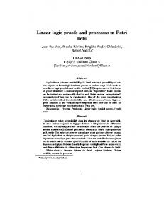
Example 3.1 Starting from the Petri net system shown in Figure 3.1 we can obtain a natural set of formulae from a fragment of Linear Logic describing each transition and the marking. We start by describing the current marking of the net by introducing one resource of type p for each token on place p and writing them as a tensor product. In our net the current marking is, therefore, A2 ⊗ C indicating the presence of two tokens on place A and one token on place C.

t u C r

A 2

s B

Figure 3.1: A simple P/T net

3.1 Encoding P/T Nets and Extended P/T Nets

C r

A

B

31

The occurrence of a transition is represented by the Linear implication. For example the occurrence of r has the effect of removing one token each from the places A and C, while producing one token on the place B. The formula A ⊗ C −◦ B reflects this behaviour.

The Linear implicational formula B −◦ A2 represents the behaviour of transition s. The two remaining transitions of the P/T net in Figure 3.1 constitute special cases where we have either no preconditions or no post-conditions. A 2

s B

These transitions are encoded by the formulae A −◦ ⊥ and 1 −◦ C, respectively, representing the fact that t can consume a token from place A and conversely that u can produce a resource of type C.

t

A

u C

As usual every transition may fire as often as desired, as long as the preconditions are satisfied. Therefore, we have to precede each formula that represents a transition by the storage operator of course (!). By putting all subformulae together we arrive at an instantaneous description of the net system:

A2 ⊗ C⊗!(A ⊗ C −◦ B)⊗!(B −◦ A2 )⊗!(1 −◦ C)⊗!(A −◦ ⊥)

32


The order in which the factors of the tensor product appear is arbitrary. In the manner outlined in the previous example it is possible to construct for every net system N (m) = N , m! = P, T, F, W, m!, its canonical formula ΨILLPN (N (m)), by forming the tensor product of its component formulae. Definition 3.2 (canonical formula for a P/T net) Let N = P, T, F, W, m0 ! be a P/T net. Then the canonical formula ΨILLPN (N ) for N is constructed as the tensor product of the following component formulae: • For each transition t ∈ T with non-empty preconditions non-empty post-conditions t • , construct 

!

pW (p,t) −◦

p∈ • t

•t

and



q W (t,q)  ,

q∈t •

• In the special cases where a transition t ∈ T has no preconditions (i.e. a source transition) construct for each such transition the formula1 

! 1 −◦





q W (t,q)  or equivalently

!

q∈t •



q W (t,q)  ,

q∈t •

• For all transitions t ∈ T without any post-conditions (i.e. sink transitions) construct the Linear Logic formula 

!

p∈ • t



pW (p,t) −◦ ⊥ or equivalently



! 

p∈ • t

⊥   pW (p,t)   ,

1 The equivalent formulae on the right hand side are only given for reference. The left hand side formulae are used in the canonical formula!

3.2 A LL Sequent Calculus for Petri Nets

33

• Construct for the current marking m and all places p ∈ P with m(p) = n, n ≥ 1 the formulae pn . Thus, for the complete marking

pm(p) .

p∈P m(p)≥1

Remark 3.3 Actually, the special cases in Definition 3.2 are superfluous, as they are incorporated in the main case by the convention that an empty premise is treated as the constant 1 and an empty consequence is treated as ⊥. They are given explicit mention just to make clear that for every transition of an arbitrary P/T net there is a translation into a Linear Logic formula.

Remark 3.4 The use of the large version of ⊗, which is indexed by some domain for the interpretation of the variables, in effect amounts to a first order calculus, i.e. large operators take the part of quantifiers. Nevertheless, we only give rules for propositional calculi, as we assume the formulae to be expanded before applying any rules. The definition of the canonical formula for a net is the foundation for the Linear Logic sequent calculus that Brown proposes in [Bro89]. The calculus and its main properties are presented in the following section.

3.2

A LL Sequent Calculus for Petri Nets

The purpose of this section is to establish a basic connection between P/T nets and Linear Logic derivations. It is shown that the occurrence sequences of P/T nets correspond in a natural way to derivations in a Linear Logic sequent calculus that may serve as an interleaving semantics the behaviour of such nets. The intuitionistic Linear Logic sequent calculus (ILL) is restricted to the necessary rules to represent the occurrence of P/T net transitions.

34

Chapter 3: Linear Logic Representation of P/T Nets A A(Identity) Γ A ∆, A B (Cut) Γ, ∆ B Γ, A, B C (⊗L) Γ, A ⊗ B C

1(1) Γ, A, B, ∆ C (Exchange) Γ, B, A, ∆ C

Γ A ∆ B (⊗R) Γ, ∆ A ⊗ B

Γ A ∆, B C ( −◦ L) ∆, Γ, A −◦ B C Γ, !A, !A B (Contraction) Γ, !A B

Γ, A B (Dereliction) Γ, !A B

Γ B (Weakening) Γ, !A B

Table 3.1: Inference rules for ILLPN The inference rules from the fragment of Linear Logic shown in table 3.1 suffice for the representation of Petri nets within an intuitionistic Linear Logic calculus. We use the two-sided version of the sequent calculus rules here, as its appearance is more natural.

Remark 3.5 The calculus given above is a fragment of the full intuitionistic Linear Logic calculus and, thus, gives an interleaving semantics for Petri nets. It is nevertheless possible to give a true concurrency semantics to Petri nets by using a multi conclusion fragment of classical Linear Logic. In the original work Brown uses a derived rule (Derel) instead of the usual Dereliction rule. The rules and their interderivability is shown below.

3.3 Simulating extended P/T Nets by Linear Logic

Γ, A B (Dereliction) Γ, !A B

←→

35

Γ, (A&1), !A B (Derel) Γ, !A B

(Dereliction) is derivable in Brown’s calculus by use of the (Weakening), (Contraction), and (&L1) rules, as shown in Figure 3.2.

A A 1 (Dereliction) (Weakening) !A A !A 1 Γ, A&1, !A B (&R) Γ, !A, A&1 B (Exchange) !A A&1 (Cut) !A, Γ, !A B (Exchange)∗ Γ, !A, !A B (Contraction) Γ, !A B Γ, A B (&L1) Γ, (A&1) B (Weakening) Γ, (A&1), !A B (Derel) Γ, !A B

Figure 3.2: Interderivability of the rules (Dereliction) and (Derel)

3.3

Simulating extended P/T Nets by Linear Logic

A soundness and completeness proof for traditional P/T nets has been given in [Bro89]. We generalize this result to the class of extended P/T nets which have an additional type of transition, namely so-called disposable transitions. Our proof works directly on the reachability relation of the nets while Brown’s uses a preorder on nets that has no immediate meaning for the net dynamics of traditional Petri nets. It is necessary in her proofs as the calculus she uses allows copies of transition behaviour

36

Chapter 3: Linear Logic Representation of P/T Nets A A(Identity) Γ A ∆, A B (Cut) Γ, ∆ B Γ, A, B C (⊗L) Γ, A ⊗ B C Γ A Γ B (&R) Γ A&B


Γ A ∆ B (⊗R) Γ, ∆ A ⊗ B

Γ, A C (&L1) Γ, A&B C

Γ, B C (&L2) Γ, A&B C

Γ A ∆, B C ( −◦ L) ∆, Γ, A −◦ B C Γ, !A, !A B (Contraction) Γ, !A B

Γ, (A&1), !A B (Derel) Γ, !A B

Γ B (Weakening) Γ, !A B

Table 3.2: Inference rules for Brown’s fragment of ILL

to be accumulated in a proof, which is not possible in the underlying net formalism. We have, therefore, opted to give the whole modified proof for our calculus and extended P/T netsystems. The proof requires special attention for the rule introducing a Linear implication, as Brown’s formalism allowed the dropping of arbitrary transitions in the preorder on nets that she defines, which is not possible when using the reachability relation instead. Following the definition of extended P/T nets we prove this theorem on derivations in ILLPN corresponding to occurrence sequences of extended P/T nets.


37

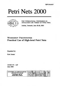
Definition 3.6 (disposable transition) A disposable transition is a transition t that may occur at most once. The occurrence rule is the same as for traditional transitions but with the effect that t will no longer be present after it has occurred.

Remark 3.7 The behaviour of a disposable transition is the same as that of the traditional transition depicted in Figure 3.3, where place C has no incoming arcs and, thus, the token residing in C cannot be replaced after it is used once. Thus, the transition can occur only once.

C

An

B ...

...

A

Bm

Figure 3.3: Disposable transition behaviour simulated by traditional transition.

38


Remark 3.8 Brown uses another net representation for the subformulae (Γ −◦ ∆)&1 that she extracts from the canonical formula by applying her (Derel) rule. The corresponding Petri net shown in Figure 3.4 has the meaning that the extracted disposable transition2 represented by (Γ −◦ ∆) may or may not occur before it is removed, i.e. the transition is not seen as a resource, since resources cannot vanish without being used. This is reflected in the formula by the use of the additive connective &, which is not resource sensitive. We favour the view of disposable transitions being pure resources as this provides a clearer semantics for the extended Petri net formalism.

C

An

B ...

...

A

Bm

Figure 3.4: Net fragment extracted by Brown’s (Derel) rule.

Remark 3.9 The finitely bounded reusable transition that is introduced in section 8.1.3 is a generalization and shorthand notation for a finite amount of identical disposable transitions. 2 Brown does not use the term disposable transition nor does she extend the traditional Petri net formalism.


39

Definition 3.10 (Extended P/T Net) A tuple P, T, D, F, W, m0 ! is called extended place/transition net or extended P/T net if 1. P is a finite set called the set of places, 2. T and D are disjoint finite sets with T ∩ P = ∅ and D ∩ P = ∅ called the sets of traditional transitions and disposable transitions, respectively. Denote by T the union T ∪D of both sets of transitions, 3. F ⊆ T × P ∪ P × T is the flow relation, 4. W : F −→IN \ {0} is the arc weight function, 5. m0 : P −→IN is the initial marking. As the transitions in D can occur at most once in a computation of an extended P/T net it is necessary to redefine the occurrence rule of P/T net systems. Definition 3.11 (enablement for disposable transitions) Let N be an extended P/T net. A transition t ∈ DN is enabled in marking m iff ∀p ∈ • t . m(p) ≥ WN (p, t) ∧ ∀p ∈ t • . m(p) + WN (p, t) − WN (t, p). If transition t is enabled in marking m it may occur. The successor marking is m with m (p) = m(p) − WN (p, t) + WN (t, p). Furthermore, the resulting net system also has a modified structure: t If N → N then N = P, T, D , F , W , m ! with D := D \ {t}, F := F \ {(x, y) | x = t ∨ y = t} and W : F −→IN \ {0}, such that ∀(x, y) ∈ F . W (x, y) := W (x, y)

40


We make use of the fragment ILLPN that does not contain the connective & used by Brown. The connective & has no immediate interpretation in the context of traditional Petri nets, which is the reason why we try to avoid using it at this stage. Furthermore, the use of & makes necessary the introduction of a preorder on net systems instead of allowing a direct argumentation on the reachability relation. We opt to use extended P/T nets instead of traditional P/T nets as the concept of disposable transitions will also play a key rˆ ole in Chapter 9 when studying possibilities of modifying net structures. We proceed by defining the canonical formula for arbitrary extended P/T net systems. Definition 3.12 (Canonical formula for extended P/T net) Let N = P, T, D, F, W, m0 ! be an extended P/T net. Then the canonical formula ΨeILLPN (N ) for N is constructed as the tensor product of the canonical formula ΨILLPN (N ) for the P/T net N := P, T, F , K, W , m0 ! where F and W are defined as in Definition 3.11 together with the following formulae as further factors: • For each transition t ∈ D with non-empty preconditions non-empty post-conditions t • , construct

pW (p,t) −◦

p∈ • t

•t

and

q W (t,q) ,

q∈t •

• In the special cases where a transition t ∈ D has no preconditions (i.e. a source transition) construct for each such transition the formula q W (t,q) , 1 −◦ q∈t •

• For all transitions t ∈ D without any post-conditions (i.e. sink transitions) construct the Linear Logic formula p∈ • t

pW (p,t) −◦ ⊥.


41

Using the canonical formula for a extended P/T net as a Linear Logic representation of the net a soundness and completeness theorem relating occurrence sequences of nets with derivations in ILLPN can be proved. We first prove a lemma on the uniqueness of the canonical formula of a given extended P/T net, then sketch the proof given by Brown and finally give a proof for our calculus ILLPN . Lemma 3.13 The canonical formula of an extended P/T net system N is unique up to isomorphism. Proof According to Definition 3.2 the canonical formula of a P/T net system is constructed as the tensor product of a number of subformulae. The same is true for extended P/T nets, which only differ from P/T nets in one additional type of factors. As the tensor product is commutative, any order yields essentially the same formula. This is due to the (Exchange) rule in the calculus, which can be permuted with the (⊗L) and (⊗R) rules yielding an isomorphism between these formulae. ✷ We establish an equivalence relation on the set of extended P/T nets, such that two nets are equivalent iff they have the same set of places and each occurrence sequence of one net can be simulated by the other. This requires a notion of reducibility among nets. Definition 3.14 (relation ≤PN on nets) Let N = P, T, D, F, W, m0 ! and N = P , T , D , F , W , m 0 ! be P/T nets with P ⊆ P . We say N is reducible to N , denoted by N ≤PN N , iff there exists an injective mapping f from P ∪ D to P ∪ D , such that the following conditions hold: 1. ∀p ∈ P . f (p) = p, 2. ∀t ∈ T . ∃t ∈ T . ( • t = • t ∧ t • = t • ) ∧ (∀(x, t) ∈ F . W (x, t) = W (x, t )) ∧ (∀(t, x) ∈ F . W (t, x) = W (t , x)), 3. ∀t ∈ D . ∀(x, y) ∈ F . [(x = t) ∨ (y = t)]⇒W (x, y) = W (f (x), f (y)),

42

Chapter 3: Linear Logic Representation of P/T Nets 4. ∀p ∈ P . m0 (p) = m0 (p).

Remark 3.15 The reducibility relation defined in Definition 3.14 secures that for two extended P/T nets N and N the relation N ≤PN holds, if a behaviour that is possible in net N is also possible in net N . This means that each disposable or traditional transition from N must have its counter-part in N . For traditional transitions it is sufficient, however, that in net N there exists one corresponding transition even if there are more than one transitions in N with the same environment. For disposable transitions there have to be at least as many similar transitions in N as in N . W.l.o.g. we have assumed the places in both nets to have the same names. This makes the constructions on the Linear Logic encodings simpler. Definition 3.16 (equivalence relation ≡PN on nets) Two P/T nets N and N are equivalent, written N ≡PN N , iff both N ≤PN N and N ≤PN N hold. Lemma 3.17 The relation ≡PN is indeed an equivalence relation. Proof It is easy to show that the relation ≡PN is (i) reflexive, (ii) symmetric, and (iii) transitive. (i) Let N := N and f = idP ∪D . Choose for every t ∈ T ∪ D the same transition in T ∪ D , i.e. t := t, to satisfy condition 2 of Definition 3.14. Conditions 1 and 4 of the same definition are satisfied as p = f (p) and m0 = m0 . So we have N ≤PN N = N . Condition 3 of Definition 3.14 is also trivially satisfied, as f is the identity mapping, i.e. ≤PN is reflexive. Thus, also ≡PN is reflexive. (ii) Conditions 2 and 4 of Definition 3.14 are defined purely by equations between components of the two nets that are in relation ≤PN , so


43

these condition are symmetric by themselves. Condition 1 fixes the restriction of f on the places of the net to be the identity mapping. From the injectivity of f it follows that D ⊆ D holds for N ≤PN N and D ⊆ D holds for N ≤PN N . Thus, ≡PN is symmetric. (iii) The transitivity of ≤PN is carried over to ≡PN by Definition 3.16. ✷ Definition 3.18 (equivalence relation ≡Ψ on canonical formulae) Two formulae ϕ and ψ are called equivalent w.r.t. the encoding of extended P/T nets iff there exist extended P/T nets N and N , such that ϕ = ΨeILLPN (N ), ψ = ΨeILLPN (ψ) and N ≡PN N . Remark 3.19 It is evident that ≡Ψ is reflexive, symmetric and transitive by the definition of ≡PN (Definition 3.16). Thus, ≡Ψ is an equivalence relation. In order to make precise the following discussion—also in later chapters—we define the logical language that will be used by giving a generating grammar. We prove that the grammar generates exactly those formulae that may stand as a extended P/T net representation. W.l.o.g. we use the set {p0n | n ∈ IN} for the propositional symbols. Definition 3.20 (grammar GePN ) We define a grammar GePN specifying all formulae that represent extended P/T net systems. Let GePN = ΣN , ΣT , S, R! with the initial symbol S included in the alphabet of non-terminals ΣN = {S, T, I, Z}, the alphabet of terminal symbols ΣT = {p, 0, (, ), ⊗, −◦ , !, 1, ⊥}. The set of rules R consists of S Z T I

−→ −→ −→ −→

S ⊗ S | T | I | !(T ) | !(I) 0 | 0Z pZ | T ⊗ T T −◦ T | 1 −◦ T | T −◦ ⊥

44


In the grammar from Definition 3.20 the names of the non-terminals are chosen to reflect the set of words they are capable of generating: I generates (simple) implicational formulae, T generates tensor products of propositional symbols, Z generates an arbitrary string of zeroes used in the names of the propositional symbols. Finally, S is the initial symbol that puts together all possible words that represent formulae, i.e. tensor products of formulae, tensor products of propositional symbols, (simple) implicational formulae, and formulae of the latter two kinds that are within the scope of the exponential connective of course (!). Lemma 3.21 The context free grammar GePN defines exactly the set of all representations of extended P/T net systems, i.e. L(GePN ) is the set containing all formulae that are equivalent to canonical formulae of extended P/T net systems up to an isomorphism on the names of places. Proof It is easy to see that Z produces any number of 0’s, i.e. L(Z) = {0}∗ . The non-terminal T produces the set of tensor products of propositional symbols L(T ) = {p}{0}∗ ({⊗}{p}{0}∗ )∗ . Similarly I generates all implications where premise and consequence are such tensor product: L(I) = L(T ){ −◦ }L(T ) ∪ {1 −◦ }L(T ) ∪ L(T ){ −◦ ⊥}. It only remains to inspect the initial symbol S. From S we can derive L(T ) by the length-preserving rule S−→T and L(I) by S−→I. The rules S−→!(T ) and S−→!(I) yield {!}{(}L(T ){)} and {!}{(}L(I){)}, respectively. The final rule to inspect is S−→S ⊗ S, thus, yielding L(S) = L(GePN ) = = (L(T )∪L(I)∪{!}L(T )∪{!}L(I))({⊗}(L(T )∪L(I)∪{!}L(T )∪{!}L(I))∗ . Thus, all words in LGePN represent nets: 1. tensor products of propositional symbols represent markings, 2. Linear implications represent disposable transitions, 3. tensor products in the scope of the exponential ! represent transitions with an empty set of input places,


45

4. Linear implications in the scope of the exponential ! represent traditional transitions, 5. finite tensor products of 1.— to 4. represent nets according to Definition 3.12 where the canonical formula for an extended P/T net is formed as the tensor product of its components, i.e. the disposable and traditional transitions as well as the marking. Names of transitions are lost in the encoding by words from L(GePN ) exactly as in the definition of the canonical formula. The other direction is also trivial. Every canonical formula of an extended P/T net system is a word from L(GePN ) by the construction of the canonical formula in Definition 3.12. ✷ Remark 3.22 For GePN there exists an equivalent regular grammar, which is not as nicely readable. The existence of such a grammar is trivial as there is no nesting of parenthesised subwords so that no counting is necessary3 . By Definition 3.16 equivalent nets consist of the same set of disposable transitions. They have for each traditional transition a matching transition that has the same behaviour, i.e. they may differ only in the number of transitions4 but not in the behaviour. Any two equivalent nets w.r.t. the relation ≡PN have the same set of places. It is clear from the definitions that equivalent nets have equivalent canonical formulae. Lemma 3.23 ϕ and ϕ are equivalent to canonical representations of extended P/T nets Nϕ and Nϕ , respectively, iff the tensor product ϕ ⊗ ϕ is a representation of an extended P/T net Nϕ⊗ϕ , equivalent to its canonical formula ΨeILLPN (Nϕ⊗ϕ ). 3

Every opening parenthesis has to be closed before the next opening parenthesis can appear in any word of L(GePN ). 4 Copies of identical transitions are allowed that only carry a different name tag are allowed.

46


Proof Let ϕ and ϕ be canonical representations of extended P/T nets Nϕ and Nϕ , respectively. Then ϕ ∈ L(GePN ) and ϕ ∈ L(GePN ) by Lemma 3.21. This means that there has to exist a derivation S G∗ ϕ and a derivation S G∗ ϕ . Then, in GePN there also exists a derivation ∗ S GePN S ⊗ S GePN ϕ ⊗ ϕ .

To prove the other direction we have to inspect the tensor prod uct ϕ ⊗ ϕ . We assume, w.l.o.g., that ϕ = i∈{1,...,m} ϕi and ϕ = j∈{n+1,...,n} ϕj . As ϕ ⊗ ϕ is a representation of an extended P/T net system, there has to exist a derivation in GePN of ϕ ⊗ ϕ . The derivation tree must have the form shown in Figure 3.5 where µi = ϕf (i) for a bijection f : {1, . . . , n}−→{1, . . . , n}.

S S

⊗

S

µ⊗...⊗µk µk+⊗...⊗µn+m Figure 3.5: Derivation tree for grammar GePN It is clear that any permutation of the word µ1 · · · µn is derivable by rearranging the order of the rules applied in the derivation. Thus, the derivation shown in Figure 3.6 must also be possible in GePN . So there ∗ ∗ exist derivations S GePN ϕ and S GePN ϕ so that by by Lemma 3.21 ϕ and ϕ are canonical representations of extended P/T netsystems. ✷ Definition 3.24 (simple tensor product, simple Linear implication) A simple tensor product is a finite tensor product p1 ⊗ . . . ⊗ pn where all pi for i ∈ {1, . . . , n} are propositional symbols.


47

S S

⊗

S

S

S

S

⇒ ϕ⊗...⊗ϕm

ϕm+⊗...⊗ϕn

ϕ

⊗

ϕ´

Figure 3.6: Derivation tree for ϕ ⊗ ϕ A Linear implication is called simple iff its premise and conclusion are simple tensor products. Lemma 3.25 Let ϕ, ϕ , ϕ and ϕ be equivalent to canonical representations of extended P/T nets Nϕ , Nϕ , Nϕ and Nϕ , respectively. Then ∗ ∗ ∗ Nϕ⊗ϕ → Nϕ ⊗ϕ if Nϕ → Nϕ and Nϕ → Nϕ . Proof By Lemma 3.23 the formulae ϕ ⊗ ϕ and ϕ ⊗ ϕ are equivalent to canonical formulae of nets Nϕ⊗ϕ and Nϕ ⊗ϕ , respectively. Any formula ψ that is known to be equivalent to a canonical formula of an extended P/T net system can be rewritten as i∈I !(τi −◦ τi ) ⊗ j∈J !(τj −◦ τj ) ⊗ τm , where I and J are suitable index sets and the formulae τk are simple tensor products of propositional symbols. The first factor represents the traditional transitions of the net, the second factor stands for the disposable transitions and the third is the subformula for the current marking. The net Nϕ⊗ϕ is obtained from Nϕ by adding for the formula ϕ the transitions represented in ϕ by exponential (simple) implicational formulae, the disposable transitions represented by (simple) implicational formulae, and by adding the tokens—and possibly appropriate places— represented by the propositional symbols in the remaining (simple) tensor product.

48


For P/T nets and extended P/T nets a monotonicity property holds with respect to reachability, i.e. the addition of transitions and tokens to an existing net preserves the enablement of transitions and computation steps, while the additional transitions and tokens are not affected. ∗ Thus, Nϕ⊗ϕ → Nϕ ⊗ϕ . The same argument applies to ϕ ⊗ ϕ , such that ∗ ∗ ∗ Nϕ ⊗ϕ holds. Altogether we get Nϕ⊗ϕ → Nϕ ⊗ϕ → Nϕ ⊗ϕ Nϕ ⊗ϕ → as desired. ✷ We treat the sequence A, B as equivalent to the tensor product A ⊗ B in the following proofs. This is perfectly legitimate as can be seen from the rules of the calculus that only allow this interpretation when moving from sequences to formulae. We proceed by giving a detailed proof of the following soundness and completeness theorems for our calculus that consists only of the multiplicative Linear Logic connectives ⊗, −◦ , and the exponential !. Theorem 3.26 If a marking m is reachable in the extended P/T net system N (m) then ΨeILLPN (N (m)) ΨeILLPN (N (m )) is provable in ILLPN . Proof ∗ N (m ). Assume N (m) → Abbreviate by the definitions N := N (m) and N := N (m ). If N = N nothing has to be shown as ΨeILLPN (N ) = ΨeILLPN (N ) automatically holds up to isomorphism by Lemma 3.13. For the proof of the remaining cases let N = N . Then there exists a finite sequence of net systems N0 , . . . , Nk , for k ≥ 1 with N0 = N and Nk = N differing only in the current marking, such that N0 → N1 → · · · → Nk−1 → Nk and Ni+1 is reached from Ni by firing exactly one of the enabled transitions of Ni for all i ∈ {0, . . . , k − 1}. Let ΨeILLPN (Ni ) = Γ⊗!(A1 ⊗ · · · ⊗ Al −◦ B1 ⊗ · · · ⊗ Bm ) ⊗ A1 ⊗ · · · ⊗ Al be the canonical formula of Ni where !(A1 ⊗ · · · ⊗ Al −◦ B1 ⊗ · · · ⊗ Bm ) is the representation of the enabled transition that takes Ni to Ni+1 . Γ is an arbitrary sequence representing the remainder of the net and current marking, not involved in the present transition occurrence. The canonical formula ΨeILLPN (Ni+1 ) of Ni+1 then must be Γ⊗!(A1 ⊗ · · · ⊗ Al −◦ B1 ⊗ · · · ⊗ Bm ) ⊗ B1 ⊗ · · · ⊗ Bm .


49

To make the derivation more readable we use the abbreviations α := A1 ⊗ · · · ⊗ Al and β := B1 ⊗ · · · ⊗ Bm . We prove ΨeILLPN (Ni ) ΨeILLPN (Ni+1 ) by giving the appropriate derivation. Identity axioms are generalized to arbitrary formulae to make the derivation as concise as possible, i.e.

ϕ ϕ

(Id)

which is derivable for an arbitrary formula ϕ is used as an additional axiom. The derivation is shown in Figure 3.7.

α α β β α, α −◦ β β !(α −◦ β) !(α −◦ β) α, α −◦ β, !(α −◦ β) β⊗!(α −◦ β) α, !(α −◦ β), α −◦ β β⊗!(α −◦ β) α, !(α −◦ β), !(α −◦ β) β⊗!(α −◦ β) α, !(α −◦ β)) β⊗!(α −◦ β) Γ Γ α⊗!(α −◦ β)) β⊗!(α −◦ β) Γ, α⊗!(α −◦ β)) Γ ⊗ β⊗!(α −◦ β) Γ ⊗ α⊗!(α −◦ β)) Γ ⊗ β⊗!(α −◦ β)

Figure 3.7: Derivation representing a transition occurrence

The (Cut) rule ensures that from the provability of ΨeILLPN (Ni ) ΨeILLPN (Ni+1 ) for 1 ≤ i < k we can deduce the provability of ΨeILLPN (N ) ΨeILLPN (N ) by applying at most k − 1 cuts to the derived sequents for the computation steps made by firing exactly one transition:

50


ΨeILL (Ni ) PN

.. .

ΨeILL (Ni+1 ) PN ΨeILL (Ni ) PN

ΨeILL (Ni+1 ) PN ΨeILL (Ni+2 ) PN

.. .

ΨeILL

PN

(Ni+2 )

(Cut)

.. . ✷ The reverse direction is provable in ILLPN only for the precedence relation given in [Bro89]. Brown defines a preorder5 * on P/T net systems and shows that for two net systems N and N the following is provable in ILLPN 6 : N * N

⇒

ΨeILLPN (N ) ΨeILLPN (N )

This corresponds to our Theorem 3.26. In addition Brown shows that if ΨeILLPN (N ) Φ is provable in ILLPN then Φ is the canonical formula of some net N , i.e. Φ = ΨeILLPN (N ), such that N * N . The latter can be proved by induction on the depth of the derivation tree, inspecting the last rule used in the derivation. We modify this in Theorem 3.27 proving a similar result for the reachability relation of extended P/T nets and provability in a slightly modified calculus ILL PN . The calculus ILL PN uses the same language as does ILLPN so that we can still use the same canonical formula ΨeILLPN (N ) for a net N . The difference lies only in the set of rules. Whereas in ILLPN we allowed unrestricted use of (Dereliction), and (Contraction) we exchange these rules for the derived rule (DeCo) while the rule (Weakening) is discarded from the calculus. The complete calculus is given in Table 3.3 for reference. 5 The preorder relates net systems N and N ’, such that N ’ is reachable by a finite number of transition occurrences from N together with—possibly—the removal of a part of the net structure. See [Bro89] for details. 6 Brown actually shows this for the calculus in Table 3.2 but the result is easily transferrable to ILLPN .

3.3 Simulating extended P/T Nets by Linear Logic A A(Identity) Γ A ∆, A B (Cut) Γ, ∆ B Γ, A, B C (⊗L) Γ, A ⊗ B C

51


Γ A ∆ B (⊗R) Γ, ∆ A ⊗ B

Γ A ∆, B C ( −◦ L) ∆, Γ, A −◦ B C Γ, !A, A B (DeCo) Γ, !A B

Table 3.3: Inference rules for ILL PN The rule (DeCo) is derivable from the (Dereliction) and (Contraction) rules by simply applying them consecutively: Γ, !A, A B (DeCo) Γ, !A B

⇐=

Γ, !A, A B (Dereliction) Γ, !A, !A B (Contraction) Γ, !A B

The reason for restricting ILLPN lies in the undesired possibilities that the rules (Weakening), (Contraction) and (Dereliction) offer. As seen in the proof of Theorem 3.26, for simulating the behaviour of extended P/T nets it not necessary to use (Weakening) at all. The (Dereliction) and (Contraction) rules are needed but only in a specific order preserved by the new (DeCo) rule. Thus, the proof of Theorem 3.26 is easily adapted to the calculus ILL PN , and so we do not sacrifice previous results for the sake of a simpler proof of the following theorem. By using ILL PN instead of ILLPN we avoid making derivations that introduce a new transition by the (Weakening) rule or exchange a traditional transition for a disposable one by an application of (Dereliction). As the resulting formulae are still representations of nets Brown has to

52


introduce a precedence relation that allows transitions to be discarded from a net, such that a net N that is precedent to N may have strictly more transitions than N . These modifications of the net structure are not reflected in the occurrence rule. Similar situations cannot occur in ILL PN and, therefore, we can prove Theorem 3.27 directly for the reachability relation on extended P/T netsand do not have to introduce a precedence relation with no immediate meaning in the context of (traditional) Petri nets. Theorem 3.27 Let N be an extended P/T net with canonical formula ϕ = ΨeILLPN (N ). If ϕ ψ is provable in ILL PN then ψ is equivalent to a canonical formula ∗ ΨeILLPN (N ) of an extended P/T net N , such that N → N . Proof Let ϕ = ΨeILLPN (N ) for an arbitrary extended P/T net N . Furthermore, assume that ϕ ϕ is provable in ILLPN . We show that ϕ is equivalent—and, thus, reducible—to the canonical ∗ formula of a P/T net N , such that N → N holds. The proof is carried out by induction over the depth of the derivation of ϕ ϕ . Basis: For the base case the depth of the derivation tree is one. This leaves only two possibilities to be considered. Firstly, the derivation tree can consist of the identity axiom and, secondly, of the axiom (1). In the former case ϕ and ϕ are identical so that ϕ clearly is the canonical formula of N = N . For the latter case interpret 1 by the empty net, consisting of an empty set of places and an empty set of transitions. As 1 is self-dual we can replace the precedent of the axiom (1), i.e. the empty sequence, by 1. By doing so we arrive at an instance of the identity axiom, as above. These are the only two possibilities for derivations of depth one. Induction hypothesis: Assume the statement from Theorem 3.27 holds for proofs of depth up to n ∈ IN, with n ≥ 2. Induction step: We inspect all eight possible cases for the last rule that may have been applied in the derivation of depth n + 1 of ϕ ϕ .


53

1. Assume the derivation ends with an application of the (⊗R) rule, Γ A ∆ B (⊗R). Γ, ∆ A ⊗ B As Γ, ∆ is synonymous with Γ ⊗ ∆ and the precedent of the conclusion is equivalent to the canonical formula of a net by assumption, the factors also represent nets NΓ and N∆ , respectively, by Lemma ∗ 3.23. Furthermore, the induction hypothesis shows that NΓ → NA ∗ → and N∆ NB hold. It remains to show that the succedent A ⊗ B is also equivalent to the canonical formula of an extended P/T netNA⊗B reachable from NΓ⊗∆ . By Lemma 3.23 the formula A ⊗ B is equivalent to the canonical formula of a net NA⊗B if A and B are equivalent to canonical formulae of nets NA and NB , respectively. This is indeed the case by the induction hypothesis. ∗ NA⊗B from the hypothesis Applying Lemma 3.25 we get NΓ⊗∆ → ∗ ∗ NA and N∆ → NB . that NΓ →

2. Assume the derivation ends with an application of the (⊗L) rule, Γ, A, B C (⊗L). Γ, A ⊗ B C This is a trivial case, as the claim holds for Γ, A, B C by the induction hypothesis and the precedent Γ, A ⊗ B of the conclusion is equivalent to the precedent Γ, A, B of the premise. 3. Assume the derivation ends with an application of the ( −◦ L) rule, Γ A ∆, B C ( −◦ L). ∆, Γ, A −◦ B C As ∆, Γ, A −◦ B is synonymous with ∆⊗Γ⊗(A −◦ B) and the precedent of the conclusion is equivalent to the canonical formula of a net by assumption, the factors also represent nets by Lemma 3.23. Applying the induction hypothesis we see that A represents a net

54

Chapter 3: Linear Logic Representation of P/T Nets ∗ ∗ NA , for which NΓ → NA holds. Similarly, N∆⊗B → NC holds for the nets represented by ∆ ⊗ B and C.

∆ ⊗ B is equivalent to the canonical formula of an extended P/T net system, as each subformula of the precedent of the conclusion is equivalent to a canonical formula of an extended P/T net system, such that ∆ and B are both equivalent to a canonical formula of an extended P/T net. Then, by Lemma 3.23 also ∆ ⊗ B is equivalent to the canonical formula of a net. A has to be either a singular propositional symbol or the simple tensor product, i.e. A represents a set of tokens. The set of places corresponding to these tokens must lie in the net ∗ NΓ⊗A , due to the fact that NΓ → NA . Similarly B represents a set of tokens corresponding to a set of places of a net structure not necessarily within the net NΓ⊗A . It is easy to show ∗ that for the net represented by A ⊗ (A −◦ B), NA⊗(A −◦ B) → NB ∗ ∗ holds. Thus, NΓ⊗(A −◦ B) → NA⊗(A −◦ B) → NB and so we have ∗ ∗ N∆⊗B → NC . The ultimate step holds by the inN∆⊗Γ⊗(A −◦ B) → duction hypothesis for the second premise of the implication introduction rule. 4. Assume the derivation ends with an application of the (Cut) rule, Γ A ∆, A B (Cut). Γ, ∆ B As Γ ⊗ ∆ must represent a net, so must Γ and ∆ on their own, by an application of Lemma 3.23. The cut formula A must also be a representation of a net, by application of the induction hypothesis, which also immediately tells us that ∆ ⊗ A and, thus, also B represent nets N∆⊗A and NB with the following properties: ∗ NΓ → NA ∗ N∆⊗A → NB

As ∆ represents a net, by applying Lemma 3.25 we get

(3.1)


∗ NΓ⊗∆ → NA⊗∆ .

55

(3.2)

The net NA⊗∆ is identical to the net N∆⊗A by our definition of ∗ equivalence (Definition 3.16). Hence, by the transitivity of → and the properties (3.2) and (3.1) we have ∗ NΓ⊗∆ → NB .

5. Assume the derivation ends with an application of the (Exchange) rule, Γ, A, B, ∆ C (Exchange). Γ, B, A, ∆ C The net represented by Γ ⊗ B ⊗ A ⊗ ∆ is identical to the net represented by Γ, A, B, ∆. By the hypothesis C is the representation of a net NC . Thus, Lemma 3.25 shows that ∗ ∗ NΓ⊗B⊗A⊗∆ → NC ⇐⇒ NΓ⊗A⊗B⊗∆ → NC .

6. Assume the derivation ends with an application of the (DeCo) rule, Γ, !A, A B (DeCo). Γ, !A B The (DeCo) rule is treated in analogy to the previous case. The assumption states that Γ⊗!A represents a net and by Definition 3.16 the equivalence NΓ⊗!A⊗A ≡PN NΓ⊗!A holds. By the induction ∗ hypothesis B represents a net NB . Thus, NΓ⊗!A → NB , by Lemma 3.25. ✷

56


Remark 3.28 It can be shown that adding (Contraction) to the set of rules of ILL PN does no harm by arguing the same way as in the last case of the proof of Theorem 3.27: Assume the derivation ends with an application of the (Contraction) rule, Γ, !A, !A B (Contraction). Γ, !A B The contraction rule can be treated like the (DeCo) rule. The assumption states that Γ⊗!A represents a net and by Definition 3.16 the equivalence NΓ⊗!A⊗!A ≡PN NΓ⊗!A holds. By the induction hypothesis B repre∗ NB , by Lemma 3.25. sents a net NB . Thus, NΓ⊗!A → We can now show that the following corollary holds for ILL PN : Corollary 3.29 Let N be an extended P/T net with the canonical formula ΨeILLPN (N ). ∗ N iff ΨeILLPN (N ) ΨeILL (N ) is provable in ILL PN . Then N → PN

Proof The “if” direction is evident from Theorem 3.26 and the fact that the only applications of (Dereliction) and (Contraction) are in the subproofs representing a transition occurrence. They appear in direct consecution and may, therefore, be replaced by the rule (DeCo). The “only if” branch follows from Theorem 3.27. The theorem only shows that for any provable sequent ΨeILLPN (N ) ϕ the formula ϕ is equivalent to the canonical formula of an extended P/T net N , such ∗ N holds. In case ϕ is not equal to ΨeILLPN (N ) up to isothat N → morphism there is another—so-called canonical—proof of the sequent ΨeILLPN (N ) ΨeILLPN (N ). ✷

3.4

Rewriting Logic

Amongst the many other possibilities of relating Petri nets to formulae of Linear Logic there is one that is worthwhile mentioning. The rewriting

3.4 Rewriting Logic

57

logic approach of Meseguer ([Mes92]) is founded on the ideas of Linear Logic and has many proximities with the Petri net encoding sketched in the previous sections. Rewriting logic has the benefit of instantly giving rise to an executable model (cf. [Mes93]). We briefly sketch the rewriting logic approach and relate it to Linear Logic. First we give a few reasons for the potential interest in rewriting logic: • Concurrent rewriting gives a real concurrency semantics for Petri nets, • The approach has the potential for a unifying framework for different approaches for modelling concurrency (e.g. transition systems, object-oriented programming, Petri nets, algebraic Petri nets,. . . ), • Rewriting Logic directly provides executable code. A rewriting engine has been efficiently implemented in Maude ([Mes93], [MW92]), which includes the functional sublanguage OBJ3. There are three kinds of modules: • functional modules: keyword fmod, e.g. NAT, • system modules: keyword mod, • object-oriented modules: keyword omod. The following example from [Mes92] shows some fragments of Maude code. Example 3.30 A functional module specifying the non-negative integers is given below. It specifies the symbol 0 as a constant of type Nat, the unary operator symbol s as a function type from Nat to Nat, and the binary infix operation symbol + as a function type from Nat2 to Nat. The intended meaning is given by the two equations, stating that 0 is the neutral element w.r.t the binary operation + that represents addition. Similarly the unary operation is defined to be the successor function by the last equation.

58

Chapter 3: Linear Logic Representation of P/T Nets fmod NAT is sort Nat . op 0 : -> Nat . op s : Nat -> Nat op + : Nat Nat -> Nat [comm] . vars N M : Nat . eq N + 0 = N . eq (s N) + (s M) = s s (N + M) . endfm

We also give an example of a system module that goes beyond equational logic, such that we can express, for instance, non-determinism:

mod NAT-CHOICE is extending Nat . op ? : Nat Nat -> Nat . vars N M : Nat . rl N ? M => N . rl N ? M => M . endm

The next example illustrates the way to model a P/T net by Maude code. It already shows the similarities to the way Petri nets can be modelled in Linear Logic.

Example 3.31 A Petri net model of a simple ticket machine and the code representing it in Maude is given below.

59

3.4 Rewriting Logic $ buy short-distance ticket with a dollar coin

buy long-distance ticket with a dollar coin

b-t2

change

b-t1 2

b’-t1

t1

4

2

q

buy short-distance ticket with two quarter dollars

b’-t2

3

t2 buy long-distance ticket with three quarter dollars

mod TICKET is subsorts Place < Marking . ops $, q, t1,t2 : -> Place . op × : Marking Marking -> Marking [assoc comm id: λ] . rl b-t1 : $ => t1×q×q . rl rl rl rl endm

b-t2 : $ => t2×q . change : $ => q×q×q×q . b’-t1 : q ×q => t1 . b’-t2 : q×q×q => t2 .

× in the Maude code corresponds to multiset union of markings. The Maude encoding expresses the commutative monoid algebraic structure of Petri nets. The example code works for concurrent computations as sketched below: → →

q×q×q×q×$×$ q×q×t1×t2×q×$ t2×t1×t2×t2×q

60


It is possible to develop a sound and complete set of rules for the multiplicative conjunctive fragment of Linear Logic including only ⊗. Further connectives can be used to represent properties of a concurrent system, but are irrelevant for its intrinsic logic. By interpreting × as ⊗ in Linear Logic and exchanging → by we are left with a Linear theory with • sequents corresponding to transitions as axioms, • rules: 1. [t] [t ] 2.

3.

(Identity),

[t1 ] [t 1 ] [t2 ] [t 2 ] (⊗), [t1 ⊗ t2 ] [t 1 ⊗ t 2 ] [t1 ] [t2 ] [t2 ] [t3 ] (Cut). [t1 ] [t3 ]

Example 3.32 A possible derivation for the ticket machine example from above is given by: q⊗q

q ⊗ q t1 $ $ t2 ⊗ q t1 t2 ⊗ q t1 ⊗ t2 ⊗ q t1 ⊗ t2 ⊗ q ⊗ $ ⊗ q ⊗ q

$⊗q⊗q

This concludes our discussion of the rewriting approach using the Maude language that—to a certain extent—has its origin in Linear Logic, as sketched above.

Chapter 4

Linear Logic Representation of Coloured Petri Nets In this chapter we extend the results on P/T nets and extended P/T nets from the previous chapter to the case of coloured Petri Nets. Section 4.1 introduces the formalism of coloured Petri nets used here. A basic relationship relying on the unfolding of coloured Petri nets is presented in section 4.2. A brief look at semantical issues for the encoding of coloured Petri nets an their extensions is taken in section 4.2.1.

4.1

Coloured Petri Nets

Coloured Petri nets have been introduced as a shorthand for P/T nets, from which they are obtained by “foldings” of transitions and places, i.e. where P/T nets have indistinguishable tokens whose meaning is emphasized only by the place they reside in, coloured Petri nets use “colours” to denote the different meaning of tokens residing in the same place. The folding of transitions leads to different occurrence modes of transitions that are often also called colours. Furthermore, transitions can occur only if a given guard function that is attached to the transition is satisfied. The guard function usually takes into account the current marking of the environment places of the respective transition. 61

62

Chapter 4: Linear Logic Representation of Coloured Petri Nets

As for P/T nets where we adapted the notations from [JV87] to better meet our needs, we have opted to slightly modify the notation from [Jen92] for our definition of coloured Petri nets. Definition 4.1 (coloured Petri net) A coloured Petri net system is a tuple CP N = P, T, F, C, C, G, V, m0 !, such that • P, T, N ! is a P/T net structure, • the colour set C is a finite collection of finite colour domains, • the colour function C : P −→C is a mapping from the places of CP N to colour sets in C, • the arc weight function V assigns to each arc (x, y) ∈ F a multiset of typed variables V (x, y), implicitly typed by the colour set of the place connected to the arc, • the guard assignment function G is a mapping from the transitions of CP N to expressions from a first order classical logic language over the set of environment variables, where for a transition t ∈ T the set of environment variables of a transition t is Vt :=

{x | x ∈ V (p, t)},

p∈ • t∪t •

• m0 : P −→bag(C(p)) is the initial marking of CP N . In Definition 4.1 the function C of a coloured Petri net assigns to each place a finite colour domain, i.e. a finite set. Whereas the colour domain of a place represents the admissible types of tokens that may occupy the place, it is sometimes said that the colour domain of a transition identifies one of the different possible occurrence modes of the transition. Our definition assigns colours only to places while the transition colour is implicit in the admissible bindings for the environment variables.

63

4.2 Linear Logic Encoding for Coloured Petri Nets

Remark 4.2 For convenience we will use a guard function that has exactly the environment variables as arguments. The bindings of the arc variables, for which the guard expression evaluates to true, determine the occurrence modes or colours of the respective transition. It is straightforward to translate the common definitions found in the literature into one another.

Definition 4.3 (binding) A binding of a transition t is a function β : Vt −→ C, such that

β(x) ∈

C(p)

p∈ • t∪t • x∈V (p,t)∪V (t,p)

and G(t)(β) is satisfied. Bt is used to denote the set of all bindings of a transition t. Definition 4.4 (enablement for coloured Petri nets) A transition of a coloured Petri net is enabled in marking m with binding β iff (V (p, t)(x) · β(x)) ≤ m(p)(β(x)). ∀p ∈ P . x∈V (p,t)

The enablement of a transition t makes possible its occurrence taking (t, β) the current marking m to its successor marking m , denoted by m −→ m , with the following property: ∀p ∈ P . m (p) = m(p)−

p∈ • t x∈V (p,t)

(V (p, t)(x)·β(x))+

(V (t, q)(y)·β(y))

q∈t • y∈V (t,q)

If the binding is of no importance for a special problem we write (t, β) t m→ m instead of m −→ m . Again, we omit mention of the transition if we are only interested in the possibility to reach a marking m from the marking m by exactly one or by an arbitrary number of transition ∗ occurrences. We denote this by m → m and m → m , respectively.

64

4.2


Linear Logic Encoding for Coloured Petri Nets

In coloured Petri nets the marking of one place is described by a multiset of typed (or coloured) tokens. Hence, the marking of an entire net requires a set of multisets each qualified by the name of the respective place (if the places have pairwise disjoint names). One advantage of coloured Petri net is that the resulting net is smaller and subnets of similar structure can easily be reused. This is simply done by folding two subnets of a P/T net and adding type (colour) restrictions to certain places. This also means that for any coloured Petri net there is a way to unfold it to derive an equivalent P/T net, for which there exists a formula in Linear Logic appropriately specifying the nets behaviour. It is well-known that a coloured Petri net can be transformed into a P/T net by replacing each place p with a set of places C(p) (one for each kind of tokens that p may hold) and replacing each transition t with a set of transitions C(t) (one for each way in which t may fire). The relationship between the new places and transitions are determined by the corresponding elements in the matrix determined by the function W (p, t). There is an obvious way, in which coloured Petri nets are representable within the same fragment of Linear Logic used in the preceding sections. The encoding used here is easily arrived at by a standard unfolding of a coloured Petri net. One problem arises when considering infinite colour domains: In the unfolding there will be infinitely many transitions for each transition of the coloured Petri net that has an incoming or outgoing arc labelled by a variable of an infinite colour domain. In this case we would have to use infinitary Linear Logic formulae as considered in [Far96]. If we restrict ourselves to finite colour domains the canonical Linear Logic formula is constructed as in the following example. Example 4.5 Consider the coloured transition depicted in Figure 4.1 and assume the multiset marking m[A] = {1, 1, 4}, m[B] = {4}, m[C] = {}, m[D] = {}

4.2 Linear Logic Encoding for Coloured Petri Nets C

A {1, . . . , 10}

65

{1, . . . , 10}

x

x’ t

y

x≥3 x = x − 1 y = y + 1

B {1, . . . , 10}

y’ D {1, . . . , 10}

Figure 4.1: Example of a coloured transition This excerpt from a coloured Petri net can be represented by A1 ⊗ A1 ⊗ A4 ⊗ B4 ⊗

!(Ax ⊗ By −◦ Cx−1 ⊗ Dy+1 ).

x∈{1,...,10} y∈{1,...,10} x ∈{1,...,10} y ∈{1,...,10} (x≥3)∧(x =x−1)∧(y =y+1)

The following slightly more complex example is taken from [Val98a]. It shows the coding of a complete coloured Petri net and makes clear the unfolding character of the Linear Logic encoding. Example 4.6 The coloured Petri net in Figure 4.2 describes the starting situation for a car race. The colour sets used for the places are: cars = {a, b}, starter = {s}, ready = {rsa, rsb}. The arc inscriptions bear multisets of variables (x, y, z) or constants (s, rsa, rsb, ssa, ssb). A Linear Logic representation of this net is given by: initial marking: first mode of t1 : second mode of t1 : first mode of t2 : second mode of t2 : coding of t3 :

p1a ⊗ p1b ⊗ p6s ⊗!(p1a −◦ p2a ⊗ p4rsa ) ⊗!(p1b −◦ p2b ⊗ p4rsb ) ⊗!(p2a ⊗ p5ssa −◦ p3a ) ⊗!(p2b ⊗ p5ssb −◦ p3b ) ⊗!(p6s ⊗ p4rsa ⊗ p4rsb −◦ p7s ⊗ p5ssa ⊗ p5ssb )

66

Chapter 4: Linear Logic Representation of Coloured Petri Nets p a

x

b

x

t

p

z

(x = a ∧ y = rsa) cars ∨ (x = b ∧ y = rsb)

cars y

z

t

(z = a ∧ y = ssa) ∨ (z = b ∧ y = ssb)

p cars

y

p

p

ready start

rsa+rsb ssa+ssb p s

s

starter

p s

t

starter

true

Figure 4.2: Starting a car race as a coloured Petri net

This representation corresponds to the coloured Petri net unfolding into a standard P/T net. A more compact way of representing the coloured Petri net from Figure 4.2 would, therefore, be p 1 a ⊗ p1 b ⊗ p 6 s ⊗

!(p1x −◦ p2x ⊗ p4y )⊗

(x=a∧y=rsa) ∨(x=b∧y=rsb)

!(p2z ⊗ p5y −◦ p3z )⊗!(p6s ⊗ p4rsa ⊗ p4rsb −◦ p7s ⊗ p5ssa ⊗ p5ssb ),

(z=a∧y=ssa) ∨(z=b∧y=ssb)

which illustrates the folding that the coloured Petri net incorporates.

67


Remark 4.7 It is easily seen from Example 4.6 above that the guard expressions are not incorporated directly in the logic, but are used as set theoretic expressions in the construction. The expansion of such formulae is always finite if the colour sets are finite. Otherwise they yield infinitary formulae. Special care has to be taken that the set theoretic expressions used in the formula constructors of the compact representation all yield decidable sets. We give a general construction of the canonical formula for a coloured Petri net along the lines of the construction in Definition 3.2. The construction is based on the general appearance of coloured transition as given in Figure 4.3. q

p V( p

t, q V(

,t)

. . .

)

. . .

t G(t)

p V(

t) i,

V( t, q

j)

pi

qj

Figure 4.3: A coloured Petri net transition

Definition 4.8 (canonical formula for a coloured Petri net) Let N = P, T, F, C, C, G, V, m0 ! be a coloured Petri net system. Define for each transition t ∈ T the sets Vt := {x | (∃p ∈ • t . x ∈ V (p, t)) ∨ (∃q ∈ t • . x ∈ V (t, q))} and C(t) :=

p∈ • t∪t •

C(p).

68


Then the canonical formula ΨILLPN (N ) for N is constructed as the tensor product of the following component formulae: (i) Construct for the current marking m and all places p ∈ P with m(p) = [[x1 , . . . , xn ]], n ≥ 1 the formulae

pm(p)(x) , x

x∈m(p)

(ii) For each transition t ∈ T construct 





β:Vt −→C(t) G(t)(β)

! 

(p∈P ) (p,t)∈F

V (p,t)(x)

pβ(x)

(q∈P ) (t,q)∈F

x∈V (t,q)

−◦

x∈V (p,t)

V (q,t)(x)  

qβ(x)

.

Thus, for the complete marking and net structure we get the following Linear Logic representation

p∈P m(p)=∅

x∈m(p)

pm(p)(x) ⊗ x



⊗

t∈T



β:Vt −→



!  C(t)

G(t)(β)

(p∈P ) (p,t)∈F

x∈V (p,t)

V (p,t)(x)

pβ(x)

−◦

(q∈P ) (t,q)∈F

x∈V (t,q)

V (q,t)(x)  

qβ(x)

.

The construction of the canonical formula for a coloured Petri net involves (i) creating a propositional symbol px for each token of type x that resides in place p of the net. In addition (ii) the structure of the net is represented by Linear implicational formulae for all possible bindings satisfying the respective guard formula of each transition. This is accomplished by building the tensor product of all the possibilities where each implicational formula is preceded by the exponential of course analogous to the case of P/T net formulae.


4.2.1

69

Extensions of Coloured Petri nets

Some problems have to be considered when trying to extend Definition 4.1 of the base formalism of coloured Petri nets. These problems are connected to the encoding of coloured Petri nets by propositional Linear Logic formulae. Disposable transitions are not as easily introduced into the coloured Petri net formalism as they were into the P/T net formalism. This is due to the fact that a coloured transition can occur in several modes, each of which has to be described by its own Linear implicational formula. The analogue to the construction on P/T nets would, thus, yield a transition that can occur at most once in each mode. A solution would be to introduce into the formula a new propositional symbol, that is present with multiplicity one as a factor in the formula and that is also present in every premise of the implicational formulae representing the different modes of the coloured transition. The introduction of such a resource that is used once the transition occurs in any one mode can simulate the behaviour of disposable transitions for coloured Petri nets, but there is, of course, a difference in quality, as the transition (the formula representing the transition) does not actually disappear. Another problem is the use of infinite colour domains, such as the set of integers, that some authors allow. This would yield an infinitary formula, which is not supported by the standard Linear Logic semantics, the coherent spaces presented in section 2.2.3. As long as the colour domains of the coloured Petri nets remain finite the Linear Logic encoding is essentially reducible to the encoding for P/T nets and, thus, the standard coherent space semantics of Linear Logic are applicable. In these cases we can use the encoding introduces in the previous section.

Chapter 5

Linear Logic Petri Nets We introduce Linear Logic Petri nets as a high-level formalism that has Linear Logic formulae as tokens in a standard net structure with arc inscriptions and guard functions. In this chapter we follow the definitions given in [Far98a] using Linear Logic formulae both as inscriptions of Petri Nets—i.e. as arc inscriptions and guards—and also as tokens that move through a system represented by a Petri net. The evolution of such tokens is determined by the rules of Linear Logic and by the occurrence rule of the net. In principle, any logic can be used in this kind of net formalism but presently we are only interested in the case of Linear Logic or fragments of Linear Logic based calculi. This is due to the strong connections between Linear Logic and Petri nets discussed in the previous chapters. Before giving a formal definition of a Linear Logic Petri net we informally specify some requirements in section 5.1. A brief discussion of the differences between value and reference semantics (section 5.3) is followed by a section on requirements for the occurrence rule follows (section 5.4).

5.1

Informal Discussion

This section aims at giving some hints as to what the occurrence rule should incorporate to make Linear Logic Petri nets a useful tool. But Linear Logic Petri nets must not be understood as a modelling tool, rather 70

5.2 Formal Definition

71

we suggest to view Linear Logic Petri nets as a formal but easily comprehensible semantics in a uniform setting for other modelling formalisms, such as high-level nets. The formalism of Linear Logic Petri nets is clearly not suited for the average user or programmer, but it is possible to build upon the definitions of Linear Logic Petri nets to give a more comprehensive interface that is translatable to the formalism presented here1 . This leads to some requirements that are incorporated in the approach of Linear Logic Petri nets and the corresponding occurrence rule. The basic concept of a (Linear) Logic Petri Net consists of the following ideas: • The use of logical formulae2 as tokens. • Token formulae are allowed to evolve while residing in a place of the underlying net structure according to the derivation rules of the calculus. No transition has to be fired for this kind of dynamic behaviour called autonomous derivation step. • Token formulae are temporarily bound to variables that constitute the arc inscriptions while a transition is executed. The binding has to respect that identical arc inscriptions have to be bound to identical token formulae residing in the respective places of the net. • Transitions are guarded by Linear Logic formulae—actually Gentzen-style sequents—including the variables from their incoming and outgoing arcs. If there exists such a binding of token formulae to arc variables that all sequents of the guard formula for a particular transition are derivable in the fragment of Linear Logic specified by the logic colour function, we say that the transition is enabled in this binding. The marking of the net is updated according to the enabling binding in case the transition decides to fire. 1

Just like nobody likes to write programs in assembler code but prefers a high-level programming language. Such a kind of programming language could be defined for different fragments of Linear Logic, such that the tokens can be described by data structures and guards by program code in this language. 2 Although formulae of Linear Logic are often viewed in this thesis in conjunction with a corresponding Petri net, this is not necessary. The definition of Linear Logic Petri nets do not rely on this interpretation.

72

Chapter 5: Linear Logic Petri Nets

5.2

Formal Definition

What follows is the basic definition of a Linear Logic Petri net. In this most general version we can use the whole classical Linear Logic calculus or restrict the calculus to any fragment of Linear Logic to be used in the inscriptions of the net or in the tokens themselves. If no mention is made of the fragment to be used, we will assume the whole of CLL to be permissible. It turns out, though, that it is useful to limit the possible behaviour in practice when studying this class of nets as a possible semantics for different high level object net concepts. Definition 5.1 (Linear Logic Petri Net) A Linear Logic Petri net LLPN = P, T, F, Λ, G, V, m0 ! consists of the following: • P, T, F ! is a net structure, where as usual we assume the sets of places and transitions are disjoint finite sets of the form P = {p1 , . . . , pn } and T = {t1 , . . . , tm } for non-negative integers n, m ∈ IN depending on the net. • The logic-colour-function Λ is a mapping from P ∪ T to fragments of Linear Logic. LΛ(p) is used to denote the set of terms that may appear as the colour of a token for place p. • V is a mapping with domain (P ×T )∪(T ×P ), such that if {x, y} = {p, t} with p ∈ P and T ∈ T , then V (x, y) is a multiset of variables from LΛ(p) . Moreover, for (x, y) ∈ F we let V (x, y) be the empty multiset. • The Linear Logic sequentss that may be used for the guard assignL ment function G : T −→2 Λ(t) of a transition t ∈ T is determined by LsΛ(t) the set of sequents over Λ(t) with variables from the set Vt of environment variables of transition t, defined by Vt :=

{x | x ∈ V (p, t)}.

p∈ • t∪t •

For any place p in the environment of transition t the set inclusion LΛ(p) ⊆ LΛ(t) must hold.


73

• A marking of LLPN is a mapping m with domain PN , such that m(p) is a multiset over LΛ(p) . m0 is the initial marking of LLPN .

Remark 5.2 Although the arc inscriptions and transition guards are defined as multisets of variables and sequents, respectively, the multiset brackets are usually omitted in graphical representations of nets. The necessity for restricting the used fragment of Linear Logic can have many reasons. Depending on the need for representing different kinds of non-determinism3 , for instance, can require the choice of different calculi for different subnets. In general, the use of calculi differing not only in the set of propositional symbols allowed within formulae will lead to confusion. Thus, it is strongly advised to disallow the use of calculi with different rules and axioms within one Linear Logic Petri net, although this is technically possible from the definition. The main problem with using the whole calculus CLL is its undecidability. Furthermore, the Linear Logic Petri net formalism will be used here for discussing the semantics of object Petri nets. While the basic object net formalisms use only elementary net systems we have already discussed an extension of P/T nets in Chapter 3 as a first step towards introducing some sort of dynamics into the structure of Petri nets. For further dynamization of object nets we will have to extend the Linear Logic calculi mentioned so far. This is done in chapter 9. For the following discussion we always assume one underlying calculus for the whole net4 . Such Linear Logic Petri nets are called uniform Linear Logic Petri nets or uLLPN for short. The logic colour function of a uniform Linear Logic Petri net assigns to each place of the underlying net the same logical calculus that is also used for the guard sequents. This will contain the whole classic Linear Logic (CLL) unless otherwise stated. 3

external vs. internal non-determinism This will be essential for giving a purely logical characterization of Linear Logic Petri nets. 4

74


Remark 5.3 One may object that the design decision of allowing autonomous derivation steps undermines a basic rule of Petri nets, namely that no action can occur unless some transition fires. We have nevertheless chosen to break this rule, as there is an easy way out: Think of an invisible transition attached to each place of the underlying net in the manner of a simple loop. Let the guard of these transitions be satisfied if and only if there is a token formula in the place and let the transition replace that formula with a derived formula according to the logic calculus.

The approach suggested in Remark 5.3 is formally executed in the definition of the non-autonomous derivation form of a Linear Logic Petri net that is used in the definition of the notion of processes for Linear Logic Petri nets on page 90, later in this chapter.

75


Remark 5.4 In some cases it may be necessary to keep a limited record of the history of the net execution. This becomes evident, for instance, when trying to model the exact behaviour of object systems from Valk’s original definition. A marking of a Linear Logic Petri net can then optionally be viewed as a pair (φ, ψ) where φ is a mapping from places of N to multisets of token formulae and ψ is map from places to multisets of interaction tags. Interaction tags are used to keep track of which synchronized transitions are fired in each copy of the token formula that concurrently moves through the net. They can be used to check whether two copies of a formula can be joined by a join transition in the sense of object systems, i.e. iff they represent an object net that has evolved in two different ways but can be described by two subprocesses that are consistently extendible to a common object net process. Let M = (φ, ψ) and M = (φ , ψ ) be markings of a Linear Logic Petri net. M ⇒M iff one of the following holds: 1. no interaction, no transition occurrence: ψ(p) = ψ (p) and φ(p) φ (p), 2. transport occurrence of t: If there is a binding β satisfying g(t)(W ( • t, t) + W (t • , t)) and ∀p ∈ P . φ(p) ≥ β(p, t) then φ (p) = β(W (t, p)) + φ(p) − β(W (p, t)) and

ψ(p) = ψ (p),

3. interaction occurrence: as above, but the satisfying formula may use some interaction tokens from ψ, which are consumed. Thus, ψ ⊂ ψ. We will not go into any more detail of this special kind of markings. For the remainder of this thesis we focus on the more general model where the interaction tokens are omitted.

76


Before proceeding with a more formal treatment of the occurrence rule for Linear Logic Petri nets we give a small example of a Linear Logic Petri net and discuss its behaviour. Example 5.5 We model a simplified version of Carl-Adam Petri’s famous fire extinguishing example with a Linear Logic Petri net.

A

B

C

Figure 5.1: Setting of the fire extinguishing example The situation to be modelled consists of a fire in location C, a source of water in location A, a path from A to C via B, and two firemen each carrying a bucket, which can be full or empty. The firemen form a chain in the sense that both only walk half way and then exchange the buckets. We use the following propositional variables: Ai , Bi , Ci E i , Fi

Fireman i is in location A, B or C, resp. The bucket that fireman i is carrying is empty, resp. full.

The first fireman is modelled by the Linear Logic formula !(A1 −◦ B1 )⊗!(B1 −◦ A1 ). This formula describes the ability to move back and forth between location A and location B. The possibility to fill an empty bucket in location A is described by the subformula (A1 ⊗E1 ) −◦ (A1 ⊗F1 ) in the sequent of t1 ’s guard. The second fireman is analogously modelled by !(B2 −◦ C2 )⊗!(C2 −◦ B2 ) and emptying the bucket at the location of the fire by (C2 ⊗F2 ) −◦ (C2 ⊗E2 ) in the guard of transition t3 . The exchange of buckets in location B is represented by !((B1 ⊗ B2 ⊗ Fx ⊗ Ey ) −◦ (B1 ⊗ B2 ⊗ Fy ⊗ Ex )), which is incorporated into the guard function—shown in a dashed box above the corresponding transition—of the Linear Logic Petri net shown in Figure 5.2.

77


The marking shown also states that the firemen occupy locations A and B, respectively. The variables underly the following constraint: x, x ∈ {A1 ⊗!(A1 −◦ B1 )⊗!(B1 −◦ A1 ), B1 ⊗!(A1 −◦ B1 )⊗!(B1 −◦ A1 ), B2 ⊗!(B2 −◦ C2 )⊗!(C2 −◦ B2 ), C2 ⊗!(B2 −◦ C2 )⊗!(C2 −◦ B2 )} represent the description of the firemen’s autonomous behavioural possibilities together with the current location whereas y, y ∈ {E1 , E2 , F1 , F2 } model the current state of one of the two buckets. x, y, (B1 ⊗ B2 ⊗ F ⊗ E ) −◦ (B1 ⊗ B2 ⊗ F ⊗ E ) x ⊗y exchange buckets

x , y

t fill bucket

x, y, (A1 ⊗ E1 ) −◦ (A1 ⊗ F1 ) x ⊗y

t

x, y

E1

t

x , y

A1 ⊗!(A1 −◦ B1 )⊗!(B1 −◦ A1 )

x, y

x, y

B2 ⊗!(B2 −◦ C2 )⊗!(C2 −◦ B2 )

x , y

empty bucket

x, y, (C2 ⊗ F2 ) −◦ (C2 ⊗ E2 ) x ⊗y

F2

Figure 5.2: Linear Logic Petri net for the fire extinguishing example

The formulae residing in the only place of the example net in Figure 5.2 have the possibility of evolving autonomously according to the Linear Logic calculus. The derivations that are possible correspond to the possibility of the firemen moving from one location to another. If both firemen occupy location B the exchange of buckets can take place by the synchronising transition t2 whose guard prevents the exchange in all cases but the one where the left fireman has a full bucket and the other carries an empty bucket. Similarly, the other transitions model the filling and emptying of the buckets. The behaviour of the net can be seen from Figure 5.3 depicting its reachability graph. Dashed arcs represent the autonomous evolution of the token formulae. These can be traversed in both directions in this example. A shorthand with an obvious meaning is used for the markings (e.g. a1e1,b2f2 denotes the marking where A1 ⊗!(A1 −◦ B1 )⊗!(B1 −◦ A1 ) together with E1 and

78


B2 ⊗!(B2 −◦ C2 )⊗!(C2 −◦ B2 ) as well as F2 are the token formulae present in the only place).

t a1f1,c2e2

a1f1,b2e2

b1f1,c2e2

b1f1,b2e2

t

a1e1,b2e2

a1e1,c2e2

b1e1,b2e2

b1e1,c2e2

t t

t

t b1f1,b2f2

a1f1,b2f2

b1e1,b2f2

b1e1,c2f2

a1e1,b2f2

a1e1,c2f2

t

t b1f1,c2f2

a1f1,c2f2

t Figure 5.3: Reachability graph for the net in Figure 5.2

The reachability graph is not completely drawn in Figure 6 in order to retain readability. It is in general possible to combine the autonomous behaviour of a token formula with the derivation forced by a transition. For instance, from node b1f1,c2f2 by transition t3 it is possible to reach the nodes a1f1,c2e2 and b1f1,b2e2 in addition to b1f1,c2e2. Similarly, also autonomous derivation steps can be combined.

In the following example we show how Linear Logic Petri nets can be used to simulate processes triggered by some event.

5.3 Value vs. Reference Semantics

79

Example 5.6 Consider the formula SU ⊗!(SU ⊗ c −◦ AU ⊗ c)⊗!(AU ⊗ c −◦ W I ⊗ c)⊗ !(W I ⊗ c −◦ SP ⊗ c)⊗!(SP ⊗ c −◦ SU ⊗ c). The Linear Logic Petri net depicted in Figure 5.4 has this formula as token formula. It models the change of seasons, with W I for winter, SP for spring, SU for summer, and AU for autumn. The only possible event is the change of season represented by the transition and the pair of triggers c and c. The guard filters out the propositional symbol c before placing the modified token formula in the only place of the net. The Figure illustrates the possible behaviour of the net, i.e. the change from winter to spring, from spring to summer, from summer to autumn, from autumn to winter, and so on.

5.3

Value vs. Reference Semantics

Although reference semantics are especially useful when combining Petri nets with modern programming languages, there are some reasons that have lead to the use of value semantics for Linear Logic Petri nets. • As Linear Logic Petri nets have a logical calculus as their “engine” it is more common not to allow references. The propositional symbols cannot be assigned a reference or pointer as this would make necessary a vast amount of changes to the calculus. • The use of reference semantics violates the principle of locality, as shown in [Val98b]. • For object Petri nets the interaction between two objects residing in the same place should be possible, but in the case of references to distant objects this is not feasible. • Reference semantics do not seem appealing for Linear Logic based system specifications, due to the resource sensitivity within the logic

80


WI ⊗!(SU ⊗c −◦ AU ⊗c) ⊗!(AU ⊗c −◦ W I⊗c) ⊗!(W I⊗c −◦ SP ⊗c) ⊗!(SP ⊗c −◦ SU ⊗c)

AU ⊗!(SU ⊗c −◦ AU ⊗c) ⊗!(AU ⊗c −◦ W I⊗c) ⊗!(W I⊗c −◦ SP ⊗c) ⊗!(SP ⊗c −◦ SU ⊗c)

x

t

SP ⊗!(SU ⊗c −◦ AU ⊗c) ⊗!(AU ⊗c −◦ W I⊗c) ⊗!(W I⊗c −◦ SP ⊗c) ⊗!(SP ⊗c −◦ SU ⊗c)

x

t y

x⊗cy⊗c

SU ⊗!(SU ⊗c −◦ AU ⊗c) ⊗!(AU ⊗c −◦ W I⊗c) ⊗!(W I⊗c −◦ SP ⊗c) ⊗!(SP ⊗c −◦ SU ⊗c)

x⊗cy⊗c

y

x

t y

x⊗cy⊗c

x

t y

x⊗cy⊗c

Figure 5.4: The change of seasons as a LLPN that again suggests a strong locality of all components participating in a derivation step. • Reference semantics have a benefit for the construction of large scale systems as parts of the system are re-usable. This benefit is sometimes seen as a disadvantage by people not directly involved in the construction process, due to a possible lack of transparency when making heavy use of referenced objects. In order to have a clear semantics, treating all tokens alike, we employ only value semantics for Linear Logic Petri nets. The simulation of reference semantics is possible in some cases, though. For such a simulation assume all referenced objects to reside in a special place that is connected

5.3 Value vs. Reference Semantics

81

to all transitions. The formulae residing in this place have to contain a unique propositional symbol as a factor. This symbol can be used as a token that represents a reference to the object anywhere in the Linear Logic Petri net. Guards can then take care of updating the referenced object as required. We give an example of such referencing of objects by a Linear Logic Petri net. Example 5.7 Figure 5.5 shows a Linear Logic Petri net that has a place labelled Obj, which is the reference object repository. For this example there is only one token formula in Obj, namely the formula B⊗C⊗!(γ −◦ γ⊗γ)⊗!(δ⊗B −◦ δ⊗D)⊗!(δ⊗C −◦ δ⊗E)⊗!(D⊗E −◦ F ). The token formula represents the P/T net depicted in Figure 5.6, which is referenced by the unique name γ. The propositional symbol δ is used as a synchronization tag. Synchronization is forced by the two transitions t2 and t3 of the Linear Logic Petri net. They make obligatory the synchronization with e1 and e2 of the net represented by the token formula, respectively. The references to the formula representing the net from figure 5.6 are singular propositional symbols, like γ in this example. The token formula to be referenced has to include the factor !(γ −◦ γ ⊗ γ), so that the guards of the net can correctly identify the referenced formula. For instance the guard of t1 in our example is G(t1 ) = [[y ⊗ x x ⊗ x ⊗ z]]. The variable x is used as the reference tag, y is the referenced formula, and z is the result of the transition occurrence, which can be bound to the same formula as y or to any formula derivable from y. G(t1 ) does not require a synchronous derivation step for the occurrence of the transition. In contrast t2 and t3 do require a synchronization. This is accomplished in the same fashion as described in section 6.3. The synchronization takes place between the “system net” transition and the

82


γ p1 x t1

y

z

x

x

p2

p3

x t2

x

x z

y

p4

t3

x

p5

y

z

C ⊗ B⊗!(γ −◦ γ ⊗ γ)⊗!(δ ⊗ B −◦ δ ⊗ D)⊗!(δ ⊗ C −◦ δ ⊗ E)⊗!(D ⊗ E) −◦ F

Obj Figure 5.5: Referencing formulae in Linear Logic Petri nets. referenced formula in such a way that the behaviour exhibited by object systems cannot occur here. In particular the two “copies” of the object cannot use the same token independently. The concept of referencing to the same object propagates the change in the object to all places containing a reference to it. For an overview of reference and value semantics for object systems, see [Val99]. The different semantics are compared and conditions are given for each to be simulated in the other. The conditions are fairly strict, such that the general conclusion to be drawn from this work is, that one should evaluate in advance, which semantics is most appropriate for

5.4 An Occurrence Rule for Linear Logic Petri nets

C

B

83

e2

e1

γ: D

E e3

F

Figure 5.6: The net represented by referenced formula. the desired modelling task, as a simulation with a net formalism having another semantics—if at all possible—will destroy many of the benefits that an object Petri net approach offers.

5.4

An Occurrence Rule for Linear Logic Petri nets

As stated in the introduction, a careful definition of the occurrence rule for a Petri net formalism is of utmost importance. In our case we aim at giving the underlying logic full control over the net by allowing as structured tokens formulae of Linear Logic and by specifying the guard expression in the same logical formalism. The main properties of a Linear Logic Petri net’s possible behaviour have already been sketched in section 5.1. More formally speaking, a marking of a Linear Logic Petri net is defined as a multiset of logic formulae, which leads to the following definition of the occurrence rule for Linear Logic Petri nets. A t-binding is an assignment of formulae to the

84


set of variables used within arc inscriptions of the arcs relevant to transition t, such that the guard G(t) is satisfied. A mapping β : Vt −→LΛ serves as such a t-binding where Vt denotes the set of environment variables of transition t. Each variable is assigned a unique formula even if it has multiple appearances in the multiset union of the arc inscriptions. Therefore, it is sufficient for β to be defined on the set of relevant variables. Definition 5.8 (binding) A binding for a Linear Logic Petri net transition t is a mapping β : Vt −→LΛ , such that β(x) ∈

p∈ • t∪t • x∈V (p,t)∪V (t,p)

LΛ(p)

and all sequents σ ∈ G(t)(β) are derivable in Λ(t). Bt is used to denote the set of all bindings of a transition t. As we are only discussing propositional calculi there is no need for unification at this point. Definition 5.9 (enablement for Linear Logic Petri net) Let LLPN = N , Λ, τ, W, m0 ! be a Linear Logic Petri net and t ∈ TN . We say t is enabled with binding β iff there exists a t-binding satisfying G(t), such that there is one occurrence of β(X) in the place p ∈ • t for each occurrence of X in W (p, t), i.e. ∀p ∈ • t . ∀X ∈ W (p, t) . m(p)(β(X)) ≥ W (p, t)(X) Instead of saying transition t is enabled with binding β we sometimes use the expression: t is enabled in colour β to stress the resemblance to coloured Petri nets. The satisfaction of a guard formula is defined as its syntactic derivability in the Linear Logic sequent calculus. An enabled transition should of course be able to fire, changing the marking of the net as follows: The formula occurrences bound to the variable of incoming arcs in a t-binding are removed from the current marking. On the other hand there will be created new instances of the formulae bound to outgoing arcs in their respective target places. Note that we are not presently considering any capacities for the places of a Linear Logic Petri net.

5.5 Processes of Linear Logic Petri Nets

85

Definition 5.10 (successor marking) Let LLPN = N , Λ, τ, W, m0 ! be a Linear Logic Petri net and let t ∈ TN be enabled with binding β. Then t may occur changing the marking m to reach the successor marking m according to the following rule for every place p in P and every variable X ∈ Vt that appears in the arc inscription of any arc connected to t: m (p)(β(X)) = m(p)(β(X)) − W (p, t)(β(X)) + W (t, p)(β(X)) In addition to the changing of a marking by firing a transition it is possible to make standard Linear Logic deductions on the terms that represent the tokens, thus, changing the marking within the same place without the need of a transition occurrence. We will call this type of dynamic behaviour an autonomous deduction step of the LLNP.

5.5

Processes of Linear Logic Petri Nets

In this section we define a notion of process for the formalism of Linear Logic Petri nets. As in traditional Petri nets a process should reflect sequentiality and concurrency for a possible computation of the net. The unfolding of a P/T net according to the chosen transition occurrences for such a computation leads to a causal net, i.e. a loop- and choice-free P/T net, that reflects precisely the causal dependencies for the present computation. We develop a similar notion of processes for Linear Logic Petri nets. The difference is, that—as with object system processes—the structure of the token cannot be disregarded. The indistinguishability of tokens in P/T nets simplified the definition of processes, considerably. For the development of a process notion it is helpful to follow Remark 5.3 given after the definition of Linear Logic Petri nets, i.e. we disallow autonomous derivation steps and in turn introduce new transitions with trivial guards that simulate autonomous derivations. We introduce the concepts by giving an example of a process for a simple Linear Logic Petri net before proceeding to the formal definition.

86

Chapter 5: Linear Logic Petri Nets y

t1 xy

x

A⊗!(A −◦ B) ⊗ (δ ⊗ A −◦ A2 )

(a)

p

p0 x

tp

xy

(b)

x

y

y

t2 δ, x y

y

t1 xy

x

y

tp0

xy

x

A⊗!(A −◦ B) ⊗ (δ ⊗ A −◦ A2 )

p

p0 x

t2 δ, x y

y

Figure 5.7: A Linear Logic Petri net (a) and its non-autonomous derivation form (b). Example 5.11 Take the Linear Logic Petri net from Figure 5.7 (a) and add for each place p an new transition tp together with arcs (p, tp ) and (tp , p), such that V (p, tp ) = [[x]] and V (tp , p) = [[y]]. Define G(tp ) = [[x y]]. Assume that the places of the net from Figure 5.7 (a) are assigned the language generated by the grammar with the following rules: S−→S ⊗ S | T | I |!(T ) |!(I) Z−→0 | 0Z T −→δZ | δZ ⊗ T T −→pZ | pZ ⊗ T I−→T −◦ T To construct a process for some computation of the net we first transform the net to its equivalent non-autonomous derivation form

87


shown in Figure 5.7 (b). From this net we can construct all possible processes like the one in Figure 5.8. An occurrence sequence of a Linear Logic Petri net in nonautonomous derivation form is given by a sequence of pairs (ti , βi ) of transitions and bindings. For the present case one of the possible occurrence sequences is given by: (t2 , {x/A⊗!(A −◦ B) ⊗ (δ ⊗ A −◦ A2 ), y/A ⊗ A⊗!(A −◦ B)}) (t1 , {x/A ⊗ A⊗!(A −◦ B), y/A ⊗ A⊗!(A −◦ B)}) (tp , {x/A ⊗ A⊗!(A −◦ B), y/A ⊗ B⊗!(A −◦ B)}) (tp , {x/A ⊗ B⊗!(A −◦ B), y/B ⊗ B⊗!(A −◦ B)}) This is a finite occurrence sequences to match the process depicted in Figure 5.8. From the process it is easily seen that all transitions occur in sequence. The modified net from Figure 5.9 allows for some concurrency, as shown in the process depicted in Figure 5.10. Note that the processes are shown together with the bindings satisfying the guards. This is done only to illustrate the steps taken by the net. Following the ideas stated in Example 5.11 we give a formal definition of processes for Linear Logic Petri nets. Remark 5.12 We denote the occurrence of transition t with binding β taking the t, β Linear Logic Petri net system from marking m to m by m −→ m .

Definition 5.13 (occurrence sequence of Linear Logic Petri nets) An occurrence sequence of a Linear Logic Petri net LLPN is a—not necessarily finite—sequence of transition/binding pairs w = (t1 , β1 ), . . . , (ti , βi ), . . .

,

such that the following conditions hold: • For all i that appear as indices in w the binding βi is defined on the environment variables Vti of transition ti ,

88


pA⊗!(A −◦ B)⊗(δ⊗A −◦ A2 ),1

t2

δ, x y

{x/A⊗!(A −◦ B) ⊗ (δ ⊗ A −◦ A2 ), y/A ⊗ A⊗!(A −◦ B)}

pA⊗A⊗!(A −◦ B),1

t1

xy

{x/A ⊗ A⊗!(A −◦ B), y/A ⊗ A⊗!(A −◦ B)}

pA⊗A⊗!(A −◦ B),2

tp

xy

{x/A ⊗ A⊗!(A −◦ B), y/A ⊗ B⊗!(A −◦ B)}

pA⊗B⊗!(A −◦ B),1

tp

xy

{x/A ⊗ B⊗!(A −◦ B), y/B ⊗ B⊗!(A −◦ B)}

pB⊗B⊗!(A −◦ B),1 Figure 5.8: A process of the net from Figure 5.7 (b)

89


tp

xy

x

y

y

x

t1 xy

y

tp0

xy

x

A⊗!(A −◦ B) ⊗ (δ ⊗ A −◦ A2 )

p

p0 t2 δ, x y

x

y,y

Figure 5.9: The net from Figure 5.7, slightly modified. pA⊗!(A −◦ B)⊗(δ⊗A −◦ A2 ),1

t2 1

δ, x y

{x/A⊗!(A −◦ B) ⊗ (δ ⊗ A −◦ A2 ), y/A ⊗ A⊗!(A −◦ B)}

pA⊗A⊗!(A −◦ B),2

xy

pA⊗A⊗!(A −◦ B),1

t1 2

t1 1

xy

{x/A ⊗ A⊗!(A −◦ B), y/A ⊗ A⊗!(A −◦ B)}

{x/A ⊗ A⊗!(A −◦ B), y/A ⊗ B⊗!(A −◦ B)}

pA⊗B⊗!(A −◦ B),1

pA⊗A⊗!(A −◦ B),3

tp1

xy

{x/A ⊗ A⊗!(A −◦ B), y/A ⊗ B⊗!(A −◦ B)}

pA⊗B⊗!(A −◦ B),2

Figure 5.10: A process showing some concurrency.

90

Chapter 5: Linear Logic Petri Nets • G(ti )βi is derivable in Λ(t), • There exist markings m0 , . . . , mi , . . . of LLPN , such that t1 , β1 t2 , β2 ti , βi m0 −→ m1 −→ m2 · · · mi−1 −→ mi · · · holds.

Definition 5.14 (process of a Linear Logic Petri net) Let w = (t1 , β1 ), . . . , (ti , βi ), . . . be an occurrence sequence of a Linear Logic Petri net LLPN = P, T, F, Λ, G, V, m0 !. A process for w is a causal net structure Nc = Pc , Tc , Fc !, which is adhered to the following construction 1. For each token formula ϕ with j instances of ϕ initially5 residing in a place p ∈ P of LLPN there exist places pϕ,1 , . . . , pϕ,j ∈ Pc . 2. For w = (t, β), w construct the following intermediate sets. (a) Add to Tc the new transition tk with

k:=

1 + max{j ∈ IN | tj ∈ Tc } if ∃j ∈ IN . tj ∈ Tc , 1 otherwise

i.e. Tc :=Tc ∪ {tk }. (b) Define the new set of places

Pc ∪

Pc := {pϕ,l , . . . , pϕ,l+m | ∃x ∈ Vt . β(x) = ϕ∧V (t, p)(x) = m}

p∈t •

where l=

max{j ∈ IN | pϕ,j ∈ Pc } 0

if ∃j ∈ IN . pϕ,j ∈ Pc . otherwise

(c) Furthermore, construct

Fc :=Fc ∪ p∈ • t {(pβ(x),ni , tk ) | i ∈ {1, . . . , V (p, t)(x)}∧ ∧ pβ(x),ni ∈ Nc ◦ ∧ ∀i, j ∈ {1, . . . , V (p, t)(x)} . i = j⇒ni = nj }∪ ∪ {(tk , p) | p ∈ (Pc \ Pc )} 5

. . . , i.e. in marking m0 of Definition 5.13, such that m0 (ϕ) = j.

5.6 Linear Logic Representation of Linear Logic Petri Nets

91

3. Let Pc := Pc , Tc :=Tc , and Fc :=Fc and continue with step 2. Remark 5.15 The construction from Definition 5.14 is finite only for finite occurrence sequences. Every finite occurrence sequence of a Linear Logic Petri net in non-autonomous derivation form can be extended to an infinite process by adding trivial transition occurrences that do not change the marking of the net. The newly introduced transitions that simulate autonomous derivations of the token formulae always allow such steps. Note also that the process for an occurrence sequence is not unique in the case of Linear Logic Petri nets.

5.6

Linear Logic Representation of Linear Logic Petri Nets

For Linear Logic Petri nets whose guard functions always have a finite number of satisfying assignments there is an obvious property: the whole Linear Logic Petri net is representable as a finite Linear Logic formula and can, thus, be used as a token in another Linear Logic Petri net. This means that such restriction on the Linear Logic Petri nets enables us to define a cascading or nested Linear Logic Petri net that has formulae representing Linear Logic Petri nets as tokens, which themselves may also have formulae representing Linear Logic Petri nets as tokens similar to the formalism of nested Petri nets ([Lom99]) presented in section 6.2. To achieve a Linear Logic representation without the use of quantifiers for an arbitrary Linear Logic Petri net we are faced with the same problem that prevented us from giving a finite formula for a CPN with infinite colour domains. In this case the set of formulae satisfying the guard function may be infinite. Thus, a transition of a Linear Logic Petri net can be an abstraction of an infinite amount of transitions in the corresponding P/T net.

92


Definition 5.16 (labelling function λ) Let LLPN = P, T, F, Λ, G, V, m0 ! be a Linear Logic Petri net and let P be the set of propositional symbols admissible for the underlying calculus Λ. Assume, w.l.o.g., that P ∩ P = ∅. The labelling function λ is an injective mapping with domain P × Λ(P ), such that

λ(p, ϕ) :=

 λ(p, ϕ ) ◦ λ(p, ϕ )       

λ(p, ϕ )

       p.ϕ

div

if ϕ = ϕ ◦ ϕ and ◦ is a binary connective of Λ(p), if ϕ = (ϕ ) and is a unary connective of Λ(p), if ϕ is a propositional symbol a of Λ(p), otherwise

Remark 5.17 By λ(p, Λ(p)) we denote the calculus Λ(p) with the modified language λ(p, LΛ(p) ). Assume the general case for a transition of a Linear Logic Petri net depicted in Figure 5.11, where the multisets of input and output places are not assumed to be disjoint. It is clear that an autonomous derivation of a sequent ϕ ψ is possible in Λ(p) (i.e. for the formula ϕ residing in place p) iff the sequent λ(p, ϕ) λ(p, ψ) is derivable in λ(p, Λ(p)). Define the multisets of input variables and output variables by the following formal sums: Vin (t)

:=

V (pi , t),

i∈{1,...,n}

Vout (t) :=

V (pi , t)

i∈{1,...,m}

or more generally Vin (t)

:=

Vout (t) :=

p∈ • t

p∈t •

V (p, t), V (p, t).

5.6 Linear Logic Representation of Linear Logic Petri Nets

ϕ,

.

.

.

ψ,

.

p

93

.

.

ϕ,k [ [x

.,x

.,y ,.. 

,g  ]]

. . .

ψ,l

]]

, ,..

]]

,g n ,x 

. ,.. 

t G(t)

 ,h

, [[y  [[y

q

. . .

,  ,.

.., y

, h

m ]]

, [[x 

ϕ,

.

.

.

.

.

.

ψ,

ϕ,kn

ψ,lm qm

pn

Figure 5.11: An example of a Linear Logic Petri net transition The guard function of a transition has the general form

G(t) =

{Γi ∆i | Γi , ∆i ∈ LsΛ(t) }

i∈{1,...,k}

for some non-negative integer k. For each token formula ϕ residing in a place p of the net we add the subformula λ(p, ϕ)—obtained by labelling the formula with the place name—to the tensor product representing the Linear Logic Petri net. The further details of the encoding given in Definition 5.18 are analogous to the encoding of coloured Petri nets from Chapter 4. Definition 5.18 (canonical formula for a Linear Logic Petri net) Let LLPN be a uLLPN. • For every transition t ∈ T construct the formula β∈Bt



!

λ(p, β(x)V (p,t) ) −◦

p∈ • t x∈V (p,t)

q∈t • x∈V (t,q)



λ(q, β(y)V (t,q) ) ,

94

Chapter 5: Linear Logic Petri Nets • For the current marking m construct

p∈P m(p)=∅

ϕ∈m

λ(p, ϕ)m(p)(ϕ) .

The construction of the canonical formula for a Linear Logic Petri net in Definition 5.18 can be infinite. Restricting the logical language LΛ(p) to a finite set is, therefore, a requirement for the possibility of applying the original coherent space semantics of Linear Logic to Linear Logic Petri nets. Another requirement for the construction to be effective is the decidability of the calculi Λ(t) used for the guards of transitions t ∈ T . For most practical purposes a finite logical language should suffice, as the number of different resources involved in each step of a process is usually finite, and their multiplicity can also be assumed to be bounded. The specification of such a language could be given in terms of a grammar, as shown for the infinite language L(GePN ) in section 3.3.

Chapter 6

Linear Logic Petri Nets versus Object Petri Nets We illustrate the use of Linear Logic Petri nets for giving semantics to some well-known high level net concepts found in different formalizations of object Petri nets. We focus on the key concepts of these formalisms, giving examples of how to represent them in Linear Logic Petri nets. Before discussing the key features in detail, in section 6.1 we take a look at the formalism of object systems introduced by Valk. In section 6.2 we give a short survey of the basic concepts of Lomozova’s nested Petri nets that have been introduced in 1999 and, interestingly, have a very close connection to Linear Logic Petri nets defined previously in [Far98a]. Following the discussion of the two object Petri net formalisms mentioned above, we give detailed constructions of Linear Logic Petri net representations for synchronization (section 6.3) and autonomous behaviour (section 6.4) and briefly discuss some issues on synchronization and concurrency in section 6.5. In section 6.6 we discuss possibilities of simulations between the Linear Logic Petri net and nested Petri net formalisms. Finally, section 6.7 introduces a further desirable feature of object Petri nets, namely the modification of its token net’s structure, and section 6.8 introduces a variant of Linear logic Petri nets, enriched with an occurrence checking mechanism. This is shown to be essential for the modelling of agent-oriented systems. 95

96

Chapter 6: Linear Logic Petri Nets versus Object Petri Nets

6.1

Elementary Object Systems

The main idea of object systems is the use of Petri net systems as tokens in a Petri net. Object systems generalize and extend task/flow systems as defined in [Val91]. For this reason a distinction is made between the so-called system net (or environment net) and the object nets (also called token nets). We focus on elementary object systems where both the system net and the token net are elementary Petri net systems. Definition 6.1 (Elementary Object System (EOS)) An elementary object system is a tuple EOS = SN, ON , ι, τ, M! where • SN = P, T, F, W ! is an elementary net structure, called system net of EOS, • ON = {ON 1 , . . . , ON n } (n ≥ 1) is a finite set of EN systems, called object nets of EOS, denoted by ONi = POi , TOi , FOi , mOi !, • ι = ρ, σ! is the interaction relation, consisting of a system/object interaction relation ρ ⊆ T × PO where PO := 1≤i≤n POi and a symmetric object/object interaction relation σ ⊆ (PO × PO ) \ idPO , • τ : W −→2{1,...,n} ∪ IN is the arc type function, and • M is an object marking as defined in definition 6.2. Definition 6.2 (object marking) The set Obj := {(ONi , mi ) | 1 ≤ i ≤ n, mi ∈ R(ONi )} is the set of objects of the EOS. An object marking (O-marking) is a mapping M : P −→2Obj ∪ IN, such that M(p) ∩ Obj = ∅ ⇒ M(p) ∩ IN = ∅ for all p ∈ P. The object marking of a place in a general object system can, thus, be either a set of pairs consisting of an object net together with its current marking or a natural number representing the number of black tokens that reside in the place. If both indistinguishable tokens and structured objects (object nets with their markings) may occupy a place it is not clear why they should not be allowed to share such a place. In order to provide for a clearer definition we prefer to view black tokens as a special

6.1 Elementary Object Systems

97

form of object net, namely a net that consists of exactly one place that carries a fixed name. Remark 6.3 We speak of unary elementary object systems if the set OS contains only one object net. In this case we abbreviate the formal representation by dropping all unneeded components. Thus, in the sequel a unary elementary object system will be written as SN, ON, ρ, M!. Definition 6.4 (process marking) Let EOS = SN, ON, ρ, µ0 ! be a unary elementary object system, with SN = PS , TS , FS , WS , mS ! and ON = PO , TO , FO , WO , mO !. Then define the following: • A process-marking (p-marking) of EOS is a partial mapping µ : P −→ PROC(ON ), such that µ is defined only on the places of the system net that hold a token and is div otherwise. The mapping µ assigns to each non-empty place p of the system net a process µ(p) of the object net. • The initial p-marking µ0 of EOS is µ0 (p):= proc(mO ) for each nonempty place p ∈ PS , where proc(mO ) is the initial process corresponding to mO . • The set of input- and output-processes of a given transition t: ⊕ t:={µ(p) | p ∈ • t ∧ µ(p) = div} and t ⊕ :={µ(p) | p ∈ t • ∧ µ(p) = div}. The preceding slightly revised definitions from [Val98b] do not cover the occurrence rule of object systems. We briefly and informally summarise the main impacts of the occurrence rule for object systems with value semantics and process markings and give the definition thereafter. The tokens in object systems may exhibit a dynamic behaviour as they are themselves Petri nets. In addition they can synchronize with one another or with the system net. Synchronization with other object nets is not in principle restricted to the case where they occupy the same

98


place. The occurrence rule for object systems is constructed to allow the distributed parallel execution of an object net in the presence of a strict fork and join structure, i.e. partially executed object nets may only be joined if their processes are compatible in the sense that they can all be extended to a valid object net process. The following definitions rely on the existence or non-existence of a least upper bound 3(M ) for a set of processes M . For the formal definition and a detailed discussion of the occurrence rule the reader is referred to [Val98b]. The extension of an elementary net process procEN = (XB , YE , ZF , φ) for a contact-free elementary net system EN = (B, E, F, C) by a transition occurrence of transition e ∈ E is denoted by procEN ◦ e. Definition 6.5 (occurrence rule for EOS) Let EOS be a unary elementary object system as in Definition 6.4. Let t be a system net transition, let e be an object net transition and let µ be a p-marking. The successor marking relation is defined by the following three cases: (i) (t, e) ∈ ρ (t,e)

1. The interaction pair (t, e) is enabled in µ, written µ−→, iff (∀p ∈ • t . µ(p) = div) ∧ (∀p ∈ t • . µ(p) = div) and 3 ( ⊕ t) ◦ e exists, i.e. all input places of t contain processes whose least upper bound exists and enables e and in addition the output places of t are empty. 2. If (t, e) is enabled in the p-marking µ then the synchronous step (t, e) can occur, thereby transforming µ into the successor p-marking µ , denoted by (µ−→µ ), where µ is defined by (t,e)

µ (p):=

 ⊕  3( t) ◦ e 

div µ(p)

for p ∈ t • for p ∈ • t otherwise

99

6.1 Elementary Object Systems (ii) ¬∃e ∈ TO . (t, e) ∈ ρ (t,+)

1. The interaction pair (t, ) is enabled in µ, written µ−→, iff (∀p ∈ • t . µ(p) = div)∧(∀p ∈ t • . µ(p) = div) and 3( ⊕ t) exists, i.e. all input places of t contain processes whose least upper bound exists and in addition the output places of t are empty. 2. If (t, ) is enabled in the p-marking µ then the transport step (t, ) can occur, thereby transforming µ into the successor pmarking µ , denoted by (µ−→µ ), where µ is defined by (t,+)

µ (p):=

 ⊕  3( t) 

div µ(p)

for p ∈ t • for p ∈ • t otherwise

(iii) ¬∃t ∈ TS . (t, e) ∈ ρ (+,e)

1. (, e) is enabled in µ, denoted by µ−→, iff for some p ∈ PS with µ(p) = div the process µ(p) ◦ e exists, i.e. e is enabled in µ(p). 2. If (, e) is enabled in the p-marking µ then the object autonomous step (, e) can occur transforming µ into the successor p-marking µ , written (µ−→µ ), where µ is defined by (+,e)

µ (q):=

µ(p) ◦ e for q = p , µ(q) otherwise

i.e. the only process affected by the step is the process residing in place p, which is extended by e.

6.1.1

A Critique of Object Systems

The idea behind the process markings is to represent fork/join structures that allow redundant actions but disallow inconsistent actions on the data represented by the token nets. This view has its right to exist for a large number of applications in workflow and other planning scenarios. On the

100


other hand there are some problems with this view, which we will discuss below. In traditional Petri nets the current state of a system is displayed by the current marking. Such a marking can only be reached through an occurrence sequence if each transition participating in the computation was enabled in the appropriate instance of the computation. Thus, the instantaneous description of a P/T net always represents a valid state of the modelled system. This principle is undermined in object systems by the occurrence rule for process markings. The instantaneous description given by the system and object net markings no longer have to represent a consistent state. This means that an observer has to see the whole net system to evaluate the information given by a marking. The isolated (local) view of a token net residing in a place does no longer provide any definite information. Figure 6.1 illustrates the situation described above for a unary elementary object system. In (a) two identical token net processes are present in two different places of the system net. A least upper bound trivially exists for these processes, such that a join transition could be enabled. Figure 6.1 (b) shows how the object net has emerged inconsistently. The process marking now has two processes, for which there does not exist an upper bound, residing in the two places. Thus, although each copy of the net cannot feel guilty of having offended against any rule, the whole system has reached an inconsistent state, that cannot be resolved. Whereas, in the previous example the global observer was always wellinformed about the consistency of the object system marking, in another example of a, probably, counter-intuitive property of object systems the choice taken in the object net is not the only reason for reaching an inconsistent state. Such a possibility is given in Figures 6.2, 6.3, and 6.4. The initial system state in question is given in Figure 6.2. The situation in Figure 6.3 is a partial deadlock. This can of course also happen in traditional P/T net systems, but it has a different impact if some basic design rules have been obeyed. In our example the object net ON2 still has the possibility to chose transition t5 and move on to place p8 .

101

6.1 Elementary Object Systems C

C

A

B

A

B

D

D

C A

C B

A

D

B D

(a)

(b)

Figure 6.1: An elementary object system

Again, emphasising the local view of object system markings there is no way for an observer in place p6 of the net in Figure 6.4 to see whether the marking of the object net residing there is still in conformity with other object net markings in distant places. The information content of the object net marking can, thus, not be estimated properly for the local observer. Only the system wide view can give evidence of consistency of the local object net markings. While in traditional Petri nets it is possible to check for a special situation represented by a particular marking, this is not possible in object systems. The traditional approach would be to introduce a transition that becomes enabled whenever the marking to be checked for is present. This transition could then occur and reset the system to a predefined state, e.g. remove the tokens from the places that represent a contradictory situation and restore (part of) the initial marking. This is no longer possible with object systems as each token has its complete history attached and this will never be cleared in any object system process. Removing such a token from some place of the system net and placing it in some other predefined place will, thus, not have the same effect as in P/T net systems, for example. In particular, if the situation reached in the object system is such, that two copies of an object system cannot take part in a join

102

Chapter 6: Linear Logic Petri Nets versus Object Petri Nets ON

t

p

p t p

t p

ON

t

p

t

p

p

t

p

Figure 6.2: A valid state of the object system.

transition occurrence of the system net due to the non-existence of a least upper bound of their processes, nothing will ever cure this as the extensions of two processes that do not have a least upper bound will always retain this property. The only solution in the case of object systems would be to start the whole system from scratch, hoping to avoid similar situations in the new run. P/T nets on the contrary allow for internal measures to be modelled in case of undesirable situations. This may be relevant for systems in which switching off the complete system is not feasible, as is the case in many industrial processes. While in industrial processes such measure might at least be possible this is no longer the case for some other models, e.g. some sociological models. A decision to nevertheless use object systems for modelling purposes requires a completely different modelling approach compared with the

103

6.1 Elementary Object Systems ON

t

p

p t p

t p

ON

t

p

t

p

p

t

p

Figure 6.3: Inconsistent object system evolution.

traditional one. In traditional Petri net modelling something like the production of a good from a finite number of resources is usually represented by a transition removing tokens from the respective resource places and in turn putting a token onto the place representing the produced good ([Rei86], page 8). Examples of such modelling can be found in the context of flexible manufacturing systems ([EGVC98]) and other production settings (e.g. [Jen97], chapter 18). Other Petri net modelling techniques also make heavy use of similar transitions, especially in coloured Petri nets ([Jen92], Chapter 7). Examples range from the software design for telecommunication systems and distributed systems (e.g. [XK98], [Jen97], [FG98]) to workflow management systems ([vdAVH97]). This cannot be

104

Chapter 6: Linear Logic Petri Nets versus Object Petri Nets ON

t

p

p t p

t p

ON

t

t

p

t

p

p

p

Figure 6.4: Possibly consistent object system evolution.

done, though, with object systems—at least not in the system net1 . While the object nets2 still allow this kind of modelling, the system net transitions can only join two (previously separated) copies of an object net or move a single object net to a different location. They can never take two different object nets and distribute them onto (different) new locations or join two different object nets to form a compound new object. 1 This becomes more awkward when nesting object systems, i.e. building a hierarchy of system/token net dependencies, such that the token net is itself system net for its tokens. No formal definitions have been established for this case, so far, and the difficulty will be the notion of process marking for nested object systems. 2 In the basic formalism without nesting the object nets are elementary net systems.


105

A change in the modelling approach and technique is not per se an unwanted feature of an object Petri net formalism. For programming methodologies there have also been significant changes as we have moved on from each generation of programming languages to its successor generation. In particular there has recently been a shift in the programming paradigm from imperative and functional programming to the new objectoriented design of programming languages (cf. [AC96] for an introduction to the theory of object-orientation). For practical reasons a shift towards object-oriented modelling is therefore favourable also in Petri nets, but the object system approach, for instance, is lacking of many aspects of objectorientation. It is of course very important to acquire a firm knowledge of simple object net formalisms that implement part of the object oriented approach. The value of object systems, nested Petri nets and Linear Logic Petri nets lies in this aspect rather than in offering a formalism that is in direct correspondence with the new programming languages. Of these programming languages there has yet much foundational work to be done and it cannot be expected that a well-understood Petri net formalism will emerge as fast as the new generation programming languages have. Nevertheless there is another reason to favour a slightly more complex—or should one say more general —formalism, allowing for different kinds of objects. It is arguable that there are real world objects that do not have a memory. Take for example a an ideal bucket3 , for whose functioning it is irrelevant how often it has been filled and emptied before its current use. For the reasons given above, at least the following types of tokens should be distinguished in any discussion of object Petri nets: • pure resources, – copyable/clonable – non-clonable • references to global objects, • fork/join process objects. 3 i.e. a bucket that does not loose any of its functionality by aging or being properly used.

106


Even with these distinguished token types there will be situations that are not representable in an appropriate way. In reality the behaviours that lead us to demand the introduction of different token types are not necessarily disjoint for each object, i.e. an object may be copyable for one process but not for another4 . Restricting the underlying system net structure to “regular fork/join structures” is possible but excludes many realistic models. Think only of an office situation where a form has to be filled in. The form might have many fields that at first sight seem to best be processed by two different staff members. For this reason two copies are made of the form. Due to some circumstances one copy is lost, but the other copy is completely filled in by one employee. Now there is only one copy left, which contains all the information needed. The second copy is neither available nor is it needed any longer. Thus, there is also no need for the join transition—matching the fork (copy) transition that occurred earlier in the process—to occur. Indeed as one of the copies has been trashed and only one copy of the form (object net) exists, there is no possibility for a join transition to occur.

6.1.2

Object System Marking and Occurrence Rule

There are, of course, many different ways to define markings of object systems according to the intuition underlying the specific model. One such possibility—process markings and extendibility of the processes in the input places of a system net transition—is discussed in [Val95], [Val98b], and [Val96b]. The solution given there is feasible in some cases of modelling but poses problems in others. It seems that a better solution would be to allow for different modes of enablement. This could be achieved by parametrization of the transitions, leading to different transition types dealing with different token types. For example it may be feasible to copy an application form (simply use a xerox machine) but it is not (yet) feasible to copy a human being or an animal, though both might be represented by a token net within an object system. 4 For instance, a passport can be copied to keep in a file a reference of the person, but the passport is not copyable in a way that passport control officers would accept.


107

The requirement to deal with different token types can be met by a formalism that is based on type theory or a typed logic. Such typed logical calculi are especially suitable for the application of logics to computational aspects, i.e. specification and verification of computer based systems or computer program. Linear Logic has often been quoted as a logic of computations in the sense that proofs in Linear Logic can be seen as executions of programs (cf. [Abr93]). The approach we pursue is a different one, although it can be enriched with a type theory at a later time. We propose to use guard functions to allow for different modes of enablement, depending on the structure of the tokens involved. Guards are a primitive of Linear Logic petri nets and the logic colour function determines the language in which the guards can be programmed. Nevertheless it is possible to simulate the object system behaviour as defined in [Val98b] by a Linear Logic Petri net with a slightly modified calculus, as explained in Remark 5.4. We give an informal discussion of some of the problems that occur with the marking and occurrence rule of object systems, before proceeding to the class of nested Petri nets, for which we compare with our formalism of Linear Logic Petri nets in more detail. Example 6.6 Assume a unary elementary object system with value semantics, i.e. process marking. Consider the object system depicted in Figure 6.5. It is easily verified that if t1 fires (transports) there is a possibility that the two copies of the object net autonomously execute different transitions leading to the situation in Figure 6.6. This situation clearly is a deadlock as there does not exist any upper bound to the two object net processes. Thus t2 is never enabled. This situation does not occur in the associated Linear Logic Petri net shown in Figure 6.8 as there is no implicit information on the processes of the token net formulae. The object net marking in Figure ILL (ON ) and 6.6 would be described by the token formulae C ⊗ Ψ PN D⊗ ΨILLPN (ON ), respectively, where ON is assumed to be the object net structure, i.e. the object net system with the empty marking, and

108

Chapter 6: Linear Logic Petri Nets versus Object Petri Nets ON C A

t

B D

SN

t

Figure 6.5: An object system with initial marking C

C A

B

t

A

B D

D

t

Figure 6.6: Deadlock situation for the net in Figure 6.5 ILL (ON ) is the canonical formula of ON extended to reflect the Ψ PN ILL (ON ) is derivable from synchronization requirement5 . But B ⊗ Ψ PN both, such that t2 would be enabled in the Linear Logic Petri net from Figure 6.7. This is shown by the derivability of the following two sequents: ILL (ON ) B ⊗ Ψ ILL (ON ) C ⊗Ψ PN PN

and

ILL (ON ) B ⊗ Ψ ILL (ON ). D⊗Ψ PN PN

Details of the derivation are left to the reader. Of course it would be possible to incorporate more restrictions on the token formulae in the guard function of t2 . In the example above, 5

A detailed discussion of synchronization follows in section 6.3

109


A⊗!(A −◦ C)⊗!(A −◦ D)⊗!(C −◦ B)⊗!(D −◦ B)⊗!(δ ⊗ B −◦ δ ⊗ A)

p

x t1 y

x y x z z

q

r x

y t2

δ⊗xδ⊗z z δ⊗y δ⊗z

Figure 6.7: Linear Logic Petri net compared with object system from Figure 6.5 it would be sufficient to restrict the derivation to token formulae that both have resource C or both have resource D but this would lead to a kind of typed net (see section 6.8 for a discussion of typed Linear Logic Petri nets and actors), i.e. the system net assumes some information on the structure of the token. Example 6.6 would pose no problems whatsoever if considered as an EOS with reference semantics. In that case the two copies of the object net become references to the same net, such that there is no possibility of contradictory actions. Another deficiency of object systems is the lack of transitions being able to distribute tokens taken from the input places to some other places. A simple example is given in Figure 6.9. Object system transitions are not capable of performing even such simple task. They can only take some tokens, construct their least upper bound, and possibly extend the process before placing this upper bound on all of its output places. This is

110

Chapter 6: Linear Logic Petri Nets versus Object Petri Nets p

A⊗!(A −◦ C)⊗!(A −◦ D)⊗!(C −◦ B)⊗!(D −◦ B)⊗!(δ ⊗ B −◦ δ ⊗ A),1

t1

rD⊗!(A −◦ C)⊗!(A −◦ D)⊗!(C −◦ B)⊗!(D −◦ B)⊗!(δ ⊗ B −◦ δ ⊗ A),1 qC⊗!(A −◦ C)⊗!(A −◦ D)⊗!(C −◦ B)⊗!(D −◦ B)⊗ tq

!(δ ⊗ B −◦ δ ⊗ A),1

tr

rB⊗!(A −◦ C)⊗!(A −◦ D)⊗!(C −◦ B)⊗!(D −◦ B)⊗!(δ ⊗ B −◦ δ ⊗ A),1 qB⊗!(A −◦ C)⊗!(A −◦ D)⊗!(C −◦ B)⊗!(D −◦ B)⊗

!(δ ⊗ B −◦ δ ⊗ A),1

t2

p

A⊗!(A −◦ C)⊗!(A −◦ D)⊗!(C −◦ B)⊗!(D −◦ B)⊗!(δ ⊗ B −◦ δ ⊗ A),2

Figure 6.8: Linear Logic Petri net process associated with the object systems from Figure 6.5 and 6.6.

seen as a disadvantage for many modelling tasks. Thus, we would favour an approach that is more flexible in this respect. The following section presents a formalism that is closely related to Linear Logic petri nets and cures some of the deficiencies of object systems, discussed above. The choice of the occurrence rule in nested Petri nets seems less arbitrary. It is more general, in that it allows many standard modelling techniques that are restricted by the definition of object systems.

111

6.2 Nested Petri Nets x

y

y

x

Figure 6.9: A transition distributing tokens in the net.

6.2

Nested Petri Nets

In [Lom99] Lomazova considers a Petri net formalism for the specification of multi-agent distributed systems. She introduces a strictly hierarchical formalism called nested Petri nets that, in the basic definition given in [Lom99], may have two levels in its hierarchy. A nested Petri net consists of a high-level system net that can have typed tokens and black tokens. The typed tokens are represented as P/T net systems—of which there may be an arbitrary but finite number—, and whose transitions carry a—possibly empty—set of labels from the labelling domain. The labelling domain contains for each label l from the countably finite set Lab an adjacent label l from the set Lab, where Lab and Lab are assumed to be disjoint sets and l:=l. The sets Lab and Lab are assumed to be the disjoint unions of labels for the system/object interaction (Labso ) and for the object/object interaction (Laboo ): Lab:=Labso ∪ Laboo ,

Lab:=Labso ∪ Laboo

The token objects in nested Petri nets are called element nets each of which has its own current marking, thus, multiple objects are considered as copies in this formalism. Element net transitions carry a set of labels to determine their synchronization partners. The system net transitions also carry labels, which are used to synchronize actions between system and element net(s). Synchronization is only possible between two element nets occupying the same place and between the system net and an element net residing in an input place of the transition to be synchronized.

112


Arcs in nested Petri nets are inscribed by expressions6 representing multisets or nested pairs of multisets of constants and variables for which there exist the following restrictions: • input arc expressions may neither contain constants nor multiple occurrences of the same variable symbol, • there are no restrictions on the expressions for output arcs. A distinction is made between four different kinds of steps in a nested Petri net: (i) Element autonomous steps can occur only if an unlabelled transition is enabled in an element net, which remains situated in the same place of the system net during the element autonomous step. (ii) Transitions of the system net that do not have a label can occur in a so-called transport step in exact analogy to the definitions given in [Val98b]. The marking of the involved element nets is not affected by this kind of step. (iii) A horizontal synchronization step requires the synchronized occurrence of two transitions from two element nets located in the same place of the system net. The transitions that synchronize in this kind of step must be appropriately labelled. (iv) A second type of synchronization is called vertical synchronization step. This step synchronizes a system net transition with a number of element net transitions, one in each element net involved in the synchronization. The transitions involved in the synchronization are fixed by appropriate labelling. 6

Expressions are formed from constant and variable symbols and two binary operations, such that a + b, denoting multiset union, and (a, b), denoting multiset pairing, are expressions if a and b are expressions. Constants are used to denote specific element nets.

6.2 Nested Petri Nets

113

Apart from the labelling7 of transitions that forces certain synchronizations there are no other restrictions for the occurrence of a transition. In particular there is no guard function for transitions of either the system net or the element net in Nested Petri nets. This is in analogy with object systems and considerably simplifies the computation of possible bindings. For nested Petri nets this means that the enablement of a transition is decidable. The basic formalism allowing only a two levels hierarchy can be extended to any finite number of levels by allowing the tokens to be not only elementary net systems but nested Petri nets. This extension requires a few restrictions on the circumstances under which a synchronization step can occur. See [Lom99] for details. It is clear that Linear Logic Petri nets allow for the same synchronization modes with respect to the token formulae as nested Petri nets do for element nets. The two possible synchronization steps involve either a system net transition and some element net transitions (item (iv) in the discussion above) or the synchronization of two element net transitions in two different element nets (as described in item (iii)). Both synchronization modes are supported by Linear Logic Petri nets. This has been shown in section 6.3. The remaining step modes (i) and (ii) can be represented in Linear Logic Petri nets by a transition with empty guard function, i.e. the expression true, and an autonomous derivation step, respectively. The occurrence rule of nested Petri nets does not pose any restrictions on the existence of an upper bound of the element net processes and, thus, directly corresponds to the occurrence rule of Linear Logic Petri nets. This means that a value semantics is used for nested Petri nets, naturally extending the value semantics of traditional P/T net systems. We denote a step of a nested Petri net by a pair (t, t) where t is a system net transition or the empty word and t is a set of element net transitions. A naming convention has to be introduced to avoid confusion between element net transitions in different copies of the same net, i.e. 7 The labelling reminds of process algebras like CCS and CSP by Milner and Hoare ([Mil80], [Hoa78]) who use similar communication mechanisms.

114


we assume w.l.o.g. that the element net transitions of all element nets be given pairwise disjoint names. We formalize the definition of enablement given in [Lom99]: Definition 6.7 (enablement for nested Petri nets) Enablement in nested Petri nets is defined for the following four cases: 1. An element transition e that has no label is enabled iff e is enabled in the P/T net system that the element net represents. We say the element-autonomous step is enabled. 2. A system net transition t having no label is enabled iff there exists a binding β of t—assigning expressions to the variables of the adjacent arc inscription—, such that each input place of t contains sufficiently many element nets, according to the binding β. We say the elementautonomous step (t, ∅) is enabled. 3. If an element net transition e has a label adjacent to a system net transition t, then the pair (t, {e}) is enabled iff the condition 1 for e and the condition 2 for t are satisfied simultaneously. If (t, E1 ) and (t, E2 ) are enabled in a marking of a nested Petri net, then: (t, E1 ∪ E2 ) is enabled iff E1 and E2 are sets of element net transitions belonging to pairwise disjoint element nets. 4. If an element transition e1 has a label matching an element net transition e2 of a second element net residing in the same place, then the pair (, (e1 , e2 )) is enabled iff both e1 and e2 satisfy condition 1 in the respective nets.

6.3

Linear Logic Petri nets and synchronization

Synchronization is one of the main features—if not the single main feature—of object systems. It is sometimes synonymously called interaction and is the only means by which the environment (net) can communicate with the objects (object nets) that “live” within that environment. There is no message passing mechanism, just simple static synchronization. By static synchronization we mean that the synchronization points

6.3 Linear Logic Petri nets and synchronization

115

as well as the nets that have to synchronize are fixed in the object system. No additional synchronizations can be added at the run-time of the object system. Two different kinds of interaction are possible in object systems: system-object interaction and object-object interaction. The former requires the object net to reside in the input place(s) of the system net transition with which the synchronization is to take place. This is the kind of interaction that has been studied in most detail, so far. The latter case—object-object interaction—involves two object nets in a synchronous computation step. The semantics has yet to be specified for general object systems. For synchronizations in the case of Linear Logic Petri nets we have opted to take a strictly local approach. This means that a synchronization of two derivation steps can only be forced by the guard function of a transition if the required formulae all reside in the local environment of the system net transition. There is a straightforward way to represent synchronization constraints in Linear Logic Petri nets based on the standard representation of transitions in Linear Logic formulae. In the same way that the places of the object net are represented as resources, i.e. propositional symbols in the logic calculus, we can force a synchronization by demanding the presence of a resource that can only be made available by the guard of the transition the synchronization shall be enforced with. Figure 6.10 shows a transition, its Linear Logic representation and the extension for the required synchronization. Example 6.8 Let us take a look at the following excerpt from an object system and construct a Linear Logic Petri net to represent the situation (as in [Val98b] the transitions to be synchronously fired are given the same label in sharp brackets in the graphical representation): The object system transitions from Figure 6.10 are modelled by the Linear Logic Petri net transition in Figure 6.11 with the guard formula G(x, y) = {δ⊗x y} and the token formula !(δ⊗A⊗B −◦ C) for the object net transition. In this example δ denotes a new propositional symbol that is not otherwise used in the model. Unfortunately this is not sufficient to

116


A

t SN:

e C

ON:

B

Figure 6.10: A SN transition interacting with an ON transition LLPN:

x

y

t δ⊗xy

Figure 6.11: An insufficient construction for Figure 6.10. grant that the transition is fired synchronously with the required derivation in the token formula. Though, the token formula can only transform A ⊗ B into C in the presence of δ, which is not possible before executing the derivation forced by the guard of transition t . On the other hand the guard formulae can be derived in the Linear Logic calculus even if the token formula residing in the input place and bound to x does not consume δ in the derivation of y, i.e. δ might still be present as a factor in the tensor product y if there is a derivation x y , such that y = δ ⊗ y . To avoid this undesirable behaviour some extra measures have to be enforced. A possible solution would be to modify the guard to {δ ⊗ Γ⊗!(δ ⊗ Σ −◦ ∆) (Γ − Σ + ∆)⊗!(δ ⊗ Σ −◦ ∆)} where the capital greek letters denote multisets treated as formal sums. In addition it has to be checked that the arc variables x and y are bound to Γ⊗!(δ ⊗ Σ −◦ ∆) and (Γ − Σ + ∆)⊗!(δ ⊗ Σ −◦ ∆), respectively8 , with Γ, Σ and ∆ consistently bound to subformulae of x and y. This kind of guard formula prevents δ from being unaffected by 8 Σ −◦ ∆ denotes some transition in the canonical formula of the net and Γ represents the remainder of the net.


117

the derivation and, thus, forces synchronization of the transition occurrence and derivation step. There may still be many possibilities to choose from just as a system net transition can have a variety of interaction partners in Valk’s interaction relation. The actual interaction partner is chosen non-deterministically. The previous example shows that the naive encoding of synchronization constraints bears a problem. A solution is given that requires significant technical measures to be taken. There is, however, a more elegant solution to the problem. The well-known mechanism of message passing may be employed here. For this approach the encoding of the token net transition whose canonical formula is !(Γ −◦ ∆) will be modified by inserting new propositional symbols δ and δ as factors of the Linear implication’s premise and conclusion, respectively. The symbol δ can be seen as a message requiring the synchronization with some transition of the Linear Logic Petri net, while the symbol δ represents a kind of acknowledgement message. The formula for the object net would, thus, contain !(δ ⊗ Γ −◦ δ ⊗ ∆). Example 6.9 Referring to the net from Example 6.8, depicted in Figure 6.10, we encode the object net transition by !(δ ⊗ A ⊗ B −◦ δ ⊗ C), where δ and δ are new propositional symbols. The Linear Logic Petri net structure is shown in Figure 6.12. No additional checking has to be done on the components of the token formula, as the presence of the acknowledgment message ensures that the synchronization has indeed taken place. The acknowledgment message is used only in the guard and is not passed through to the successor marking, thereby making possible also successive synchronizations with the same message handle. In general, we define for each pair (ts , to ) ∈ ρ of system and object net transition in the interaction relation two unique new propositional symbol δ(ts , to ) and δ(ts , to )—not corresponding to a place name of either net— called the message handles for synchronization of ts and to .

118

Chapter 6: Linear Logic Petri Nets versus Object Petri Nets LLPN:

x

y

t δ⊗xδ⊗y

Figure 6.12: Synchronization guard of a LLPN transition Let ϕ be a canonical formula of an extended P/T net N residing in place p of a Linear Logic Petri net LLPN , as shown in Figure 6.12. The synchronization of the transition t of LLPN with a synchronization transition t with message handle (δ, δ) in the net corresponding to the token formula is represented by a transition with the guard function: G(t) = {δ ⊗ x δ ⊗ y}. Another, perhaps even easier, possibility is the restriction of the logic language for the places of the net, which works in some cases. If the interaction symbols, like δ, are not allowed outside the scope of a Linear implication in token formulae residing in a place p, then the synchronization step is forced by this restriction, only. In addition to the synchronization of a system net transition and an object net transition there are at least two more synchronization modes that might be interesting for object systems: • Firstly, there is no reason not to allow the synchronization of more than one token net with the same system net transition. This can be accomplished by forcing all transitions of {t | ∃x . (t, x) ∈ ρ∨(x, t) ∈ ρ} to synchronize. For a simulation of this behaviour by Linear Logic Petri nets, it is sufficient to extend the construction outlined above for each such set. • Secondly, the synchronization among token nets is also desirable. This synchronization mode is also propagated by Valk, but has not yet been formally treated. It is worth mentioning, however, that extreme care has to be taken when formalising this kind of synchronization, as a too liberal definition may easily lead to a violation

119

t1

t2

t1

t2

t1

t2

2

t1

t2

t1

t1

2

2

2

2

2

t2

t2

t2

2

t2

(a)

(b)

(c)

t1

t2

t1

2

t1

t2

t1


(d)

Figure 6.13: Violation of the principle of locality by an object/object interaction of an object net with its own copy.

120

Chapter 6: Linear Logic Petri Nets versus Object Petri Nets of the principle of locality. Figure 6.13 gives an example of what should not be possible. The example shows part of an object system that in effect is a synchronization of two transitions of the same object net. As the synchronous step leads to one copy of the object net having fired transition t1 and the other having fired t2 . The processes are still compatible and a least upper bound exists so that t 2 can reunite the two copies. It may be argued that such a behaviour is perfectly admissible, although a transition can influence not only its direct environment but also some distant parts of the net. In effect a synchronization of two elementary object net transitions can be seen as temporarily9 glueing the involved transitions together.

Both of these synchronization modes can be simulated by Linear Logic Petri nets by simple extensions of the constructions discussed above. To avoid the undesired behaviour mentioned in the latter item is not straightforward, as Linear Logic Petri nets cannot distinguish between two identical token formulae that have emerged as copies of one original formula and two formulae that do not share a common ancestor.

6.4

Autonomous Behaviour

For object systems two kinds of autonomous behaviour can be distinguished: object autonomous transition occurrences and system autonomous transition occurrences. The latter are called transport in [Val95], [Val98b], and [Val96b] and can easily be modelled in Linear Logic Petri nets by transitions whose guard formula is the constant true, i.e. the guard formula is x x and all arcs connected to the transition bear the inscription x only. Object autonomous transitions on the other hand are modelled by autonomous deduction steps within a Linear Logic Petri net. Figures 6.14 and 6.15 show both kinds of autonomous object Petri net transition occurrence and the equivalent Linear Logic Petri net steps. 9 The transitions are not permanently glued together, as there may exist more than one synchronization pair involving some transition.

121

6.5 Object Petri Nets and Concurrency

A

obj

ect au evo tono m lut ion ous

rt spo

ran

B

t

B

A ect au evo tono m lut ion ous

B

obj

A

ort

nsp

tra

A

B

Figure 6.14: Autonomous Behaviour in object Petri nets

6.5

Object Petri Nets and Concurrency

In an Object Petri net formalism two or more objects in distant locations should be able to act independently. Indeed, there should not even be the possibility for distant objects to communicate directly with each other. Synchronization is assumed to be possible only locally, between to objects residing in the same place or between an object and a system net transition in whose environment the object resides. Thus, in object Petri nets concurrent autonomous object actions should be allowed as well as concurrent transports. Take Figure 6.14 as an example: Both system net and object net transitions are concurrent, i.e. the object Petri net can evolve in one step to the marking shown on the right hand side, as illustrated by the dashed line. An analogous behaviour is possible in Linear Logic Petri nets as shown in Figure 6.15. Concurrency and sequentiality in Linear Logic Petri nets is displayed in the possible processes according to Definition 5.14. Concurrency in the

122


x

ort

sp ran

A⊗!(A−◦B)

y

xy

t

A⊗!(A−◦B)

obj

ect a der utono iva m tio ous n x

x xy

y

y

obj

ect a der utono iva m tio ous n

B⊗!(A−◦B)

ort

nsp

tra

x

y

xy

B⊗!(A−◦B)

xy

Figure 6.15: Autonomous Behaviour in Linear Logic Petri nets

system net is directly reflected in the net structure of Linear Logic Petri nets. Equally, concurrency in the object net is reflected in Linear Logic Petri nets. The calculus for our translation implements an interleaving concurrency semantics for the token formulae. Other Linear Logic calculi, called multi-conclusion calculi ([Mil96]), can be used to implement real concurrency semantics. Independent token formula derivations are concurrent in Linear Logic Petri nets, just as independent object autonomous steps are concurrent in object Petri net formalisms, such as object systems and nested Petri nets, for example. Concurrency of independent object and system net transitions is also reflected by the derivations possible when firing a Linear Logic Petri net transition.

6.6 Linear Logic Petri Nets vs. Nested Petri Nets

6.6

123

Linear Logic Petri Nets vs. Nested Petri Nets

As Linear Logic Petri nets follow a different paradigm than do object systems, a direct translation would require a great amount of technicalities that do not give any substantial insight to the modelling of object Petri nets. With the reservations against some of the foundations of object systems, already expressed in the previous sections, we have chosen a slightly different Petri net formalism, which we have introduced in section 6.2, for a direct comparison: nested Petri nets. In te following sections we sketch how to translate nested Petri nets into Linear Logic Petri nets (section 6.6.1) and show that the reverse translation is also possible for a subclass of Linear Logic Petri nets (section 6.6.2. Finally we comment the possibility of translating nested Petri nets into Linear Logic formulae in section 6.6.3.

6.6.1

LLPN Representation of Nested Petri Nets

We develop in this section an encoding of nested Petri nets in Linear Logic Petri nets. We first introduce the extended canonical formula for a transition and for a net to take account of the synchronization labels of the nested Petri net. The definition follows the ideas introduced in section 6.3.

Remark 6.10 As with object systems we call a nested Petri net elementary system net and the element nets are elementary net systems. It thermore called unary if there is only one element net in the marking. This does not prevent the nested Petri net to produce of the element net during its computation.

if the is furinitial copies

124


Definition 6.11 (extended canonical formula) The extended canonical formula of a P/T net N = P, T, F, W, m0 ! with synchronization labels is defined by the tensor product of the following factors10 : • For each transition t ∈ T with empty set of labels, construct the factor  

!

pW (p,t) −◦

p∈ • t

q W (t,q)  ,

q∈t •

• For each transition t ∈ T with non-empty set of labels {l1 , . . . , ln }, construct the factor 

!

i∈{1,...,n}

li ⊗

pW (p,t) −◦ li ⊗

p∈ • t



q W (t,q)  ,

q∈t •

• Construct for the current marking m and all places p ∈ P with m(p) = n, n ≥ 1 the formulae pn . Thus, for the complete marking

pm(p) .

p∈P m(p)≥1

Theorem 6.12 For every unary elementary nested Petri net N PN without constants in arc inscriptions, there exists a canonical Linear Logic Petri net system LLPN N PN , such that the token formula is the canonical representation of the element net of N PN . Furthermore, there is a correspondence (bijection) between the transitions of N PN and LLPN N PN , such that the occurrence sequences of the system net and the Linear Logic Petri net coincide. Proof Sketch The idea for constructing a Linear Logic Petri net corresponding to the 10 As usual, w.l.o.g., assume the set of synchronization labels to be disjoint with the set of the place names.

125


nested Petri net is to simply take the system net as the basic structure for the Linear Logic Petri Net and mark the single place that is marked in the initial marking by the extended canonical formula for the object net. Then define guards for the transitions of the Linear logic Petri net corresponding to the transition labels of the nested Petri net. More formally this is expressed by the following construction: Let P, T, F, V, L! be the structure of the nested Petri net’s system net, where P, T, F ! is a Petri net structure, V is a mapping of the places to sets of variables11 , and L is a labelling function assigning to each transition a finite set of labels. For each transition t ∈ T and each label l ∈ L(t) construct a transition tl in the Linear Logic Petri net with the guard G(t) defined as follows: G(t):={l ⊗

x∈Vin (t)

x l⊗

y}

y∈Vout (t)

The transition tl is enabled iff there exists a binding of the input and output variables, such that all input formulae contain the adjacent synchronization label as message handle, according to section 6.3. Synchronization can be between the system net transition and any finite number of element net transitions, according to the set of variables Vt of the arcs connected to the system net transition of the nested Petri net. The arc inscriptions according to V can be taken without modification, as they allow only variables and are restricted to sets. This is a strict subclass of the arc inscriptions possible in Linear Logic Petri nets. From the construction it is clear that a transition t of the nested Petri net is is enabled in a vertical synchronization step with label l iff the transition tl of the Linear Logic Petri net transitions is enabled in the Linear Logic Petri net system with the extended canonical formula of the element net. ✷

11 Sets of variables suffice, as nested Petri nets do not allow the same variable to occur more than once on the set of input arcs of a transition.

126


Remark 6.13 Theorem 6.12 excludes constants as arc inscriptions. With the constructions introduced in section 6.8 we can use Linear Logic Petri nets with occurrence checking to model the full bandwidth of nested Petri nets. The use of constants in arc inscriptions is not needed for many applications, but is added in [Lom99] to model recursive computations, i.e. computations where the system net creates an instance of itself as an element net in one of its places. This element net can then create another copy of the system net in one of its places, and so on. Definitions are not given in [Lom99] but it is straightforward to model this behaviour with Linear Logic Petri nets as long as the nested nets are P/T net systems.

Remark 6.14 When considering nested Petri nets whose system net is not elementary, there is an additional need to model horizontal synchronization steps, i.e. synchronization between element nets. This requires the introduction of additional transitions attached to each place of the net. These transitions work like the transitions introduced earlier in the definition of Linear Logic Petri nets in non-autonomous derivation form, for making explicit autonomous derivation steps. Here the transitions have to check the presence of adjacent labels in two token formulae residing in the same place. It is stated in the definition in [Lom99] that horizontal synchronization is restricted to the synchronization of two element nets. Without a similar restriction a representation would not be possible in Linear Logic Petri nets as the synchronization of an unlimited number of element nets would require an infinitary construction of transitions and guards for each synchronization label. The construction sketched above works equally well, if the nested Petri net is not unary. Without great efforts, the constructions can also be generalized to the case where the element nets are arbitrary P/T net systems.


127

For a completely formal translation, the definitions given by Lomazova in [Lom99] would have to be given with more formal rigour. The principle of the translation is, however, clear from the discussion above.

6.6.2

Nested Petri Net Representation of LLPNs

For the simulation of Linear Logic Petri nets by nested Petri nets some restrictions have to be enforced on the Linear Logic Petri net. Firstly, it is not permissible in nested Petri nets to have multiple occurrences of the same variable on one or more input arcs of a transition. Secondly, there are no guard functions in nested Petri nets. The former restriction is easily checked for a Linear Logic Petri net, but the latter requires the guard to have a special form, that is representable in nested Petri nets. Definition 6.15 A guard function of a Linear Logic Petri net is in nested Petri net form (NPN form) iff it consists only of sequents, which satisfy one the following conditions: • The guard sequent is of the form x x (transport step), • the guard sequent is of the form

i∈I

l ⊗ xi l ⊗ yi for a suitable

index set I (vertical synchronization step), • if • t = t • is the singular set containing a single place and the guard has the form {l ⊗ x l ⊗ x, l ⊗ y l ⊗ y} (horizontal synchronization step). Proposition 6.16 For any Linear Logic Petri net for which the following conditions hold there exists a corresponding nested Petri net. • the initial marking consists of a formula that is an extended canonical form of some P/T net system, • the guard functions of the underlying net system are in nested Petri net form.

128


The construction of a nested Petri net from a Linear Logic Petri net that adheres to the constraints is done using the reverse technique from the proof of Theorem 6.12.

6.6.3

Nested Petri Nets as formulae

The discussion of Linear Logic Petri nets in Chapter 5 has shown that for every Linear Logic Petri net with decidable underlying logic and finite logical language there exists a Linear Logic representation. For nested Petri nets without constants in the arc inscriptions this means that a Linear Logic representation is possible in many cases: • Unary elementary nested Petri nets have a representation as a Linear Logic formula, as there is only one elementary net structure that appears as element net and the capacity of each system net place is one. Thus, there exists a finite representation in Linear Logic, based on the standard encoding of P/T net systems. Horizontal synchronization is not possible in all nested Petri net formalisms that have an elementary system net. • Elementary nested Petri nets may contain a finite amount of different element nets. As these are all representable as Linear Logic formulae and the restriction on the capacity of the system net remains, we are again able to give a finite representation. • Generalized elementary nested Petri nets have arbitrary P/T net systems as element net, but the system net is still an elementary net system. This situation yields a finite Linear Logic representation only if the element nets have a finite reachability set. Otherwise the set of bindings for the system net transitions may become infinite. • Arbitrary nested Petri nets allow horizontal synchronization, that is not possible in elementary nested Petri nets, due to the capacity restriction implicit in the system net. As the horizontal synchronization is limited to two element nets, we can also retrieve a Linear Logic formula for this case. The same restriction on the reachability set of the element nets, as in the previous case, has to apply for

129

6.7 Modifying Net Objects

a finite Linear Logic formula representing the nested Petri net to exist.

6.7

Modifying Net Objects

Taking Petri nets as token objects displays some kind of dynamics within the tokens but there is a possibility of having even more dynamic tokens, namely tokens that change not only their state but also their structure. A structural change of an object net—which is not possible in object systems—could mean that some transition of the object net is removed, replaced, or added during the system net execution. Example 6.17 Suppose it is possible to exchange some resource A for another resource B only once and that subsequent exchanges require to double the previously exchanged amount of A’s to receive still only one B. A possibility of modelling this situation is to modify the exchanging device/transition after each occurrence. The transition takes a formula that represents a net and has a transition as substructure transforming it to another transition. The transformation is suggested in Figure 6.16.

A

B

t

⇓ 2

t

A

B

Figure 6.16: A system net modifying it’s object net

130


This kind of behaviour can be expressed by the Linear Logic Petri net in Figure 6.17 with the guard function g(x1 , x2 , y1 , y2 ) = [x1 , x2 , (Γ −◦ ∆) −◦ (Γ2 −◦ ∆) y1 , y2 ] if x1 = Γ −◦ ∆ and x1 = y1 with Γ and ∆ variables. The object net systems are separated in this Linear Logic Petri net into a structural dynamic part (exchange rate) and a classic dynamic part (resources). To ensure that the derived token formulae are laid into the desired places, some kind of occurrence check or pattern matching is required (see the following section).

y1

x2

A −◦ B

A x1

exchange rate

y2

g(x1 , x2 , y1 , y2 )

resource

⇓

y1

x2

A ⊗ A −◦ B

B x1

exchange rate

g(x1 , x2 , y1 , y2 )

y2

resource

Figure 6.17: A Linear Logic Petri net for the net in Figure 6.16

In a similar fashion it is possible to check for the existence of any kind of subformula and simply consuming it by executing a transition. The conditional or unconditional generation/production of some subformula is also possible as discussed in section 6.8.

A⊗!(A −◦ B)

x

y g(x, y )

⇓ x

y g(x, y )

B⊗!(A ⊗ A −◦ B)

Figure 6.18: A more literate translation.

6.8 Linear Logic Petri nets with occurrence check

131

A more literal translation into a Linear Logic Petri net is shown in Figure 6.18 together with the guard function: g(x, y) = [x⊗!(α −◦ β) −◦ !(α2 −◦ β) y] if x = Γ ⊗ α⊗!(α −◦ β) , y = Γ ⊗ β⊗!(α −◦ β) and x = y.

Remark 6.18 Note that the discussion above does not take into consideration what kind of structural changes may be desirable. This is left totally to the modeller. The only purpose for this section was to show that whatever restrictions might be imposed on the modifications, it is in principle possible to give a clear-cut semantics by means of Linear Logic Petri nets. We will take a closer look at structural net modifications in chapter 9 taking into consideration some of the peculiarities of the Linear Logic Calculus.

6.8

Linear Logic Petri nets with occurrence check

In the previous sections it has been suggested that pure logical derivations are not sufficient to model the exact behaviour of object systems. Other modelling tasks, such as the modelling of agent-oriented distributed systems, require a kind of occurrence checking to be performed on the mobile objects. A simple equational theory can be used to broaden the scope in which Linear Logic Petri nets can give precise semantics to such high-level net formalisms. For this reason we introduce a superclass of Linear Logic Petri nets called OLLPN , which adds some basic axioms for equivalence relations in order to make it possible to check for the occurrence of subformulae. For this reason guards are enriched in Linear Logic Petri nets with occurrence check to include a set of equations as additional conditions. Although, in some situations it is possible to circumvent occurrence checking by restricting the logic colour of the places in the net, it is

132


sometimes necessary to have extra control over the transition steps. This is desirable, for instance, for agent oriented Petri nets or actor nets in which the token objects are actors/agents that pass messages in a predefined manner. We won’t go into any details of features that agent oriented Petri net approaches have to include but we will show an example of such a net. The example is only intended to motivate the necessity of the occurrence check feature in OLLPN . The main use of the occurrence check is the possibility of guaranteeing that the actors that want to communicate have the general form that actors are supposed to have. This clearly includes the existence of input and output ports for the messages being communicated. The system net then has to implement the communication protocol. Thus, in the following example the actors change their state according to the basic rules of communicating, e.g. a message has to reside in the output port of the sender before being sent and afterwards has to be in the in port of the receiver. The possibility of transmission errors is not taken into account in this simplistic example. Example 6.19 Figure 6.19 shows on the left hand side a possible graphical representation of an excerpt from an agent net, i.e. an extension of coloured Petri nets with nets as arc inscription. On the right hand side a Linear Logic Petri net with occurrence check is shown that gives the precise semantics if g(x1 , x2 , y1 , y2 ) has the following equations as condition x1 y1 x2 y2

= = = =

N1 ! ⊗ INΓ1 ⊗ OU T∆1 ⊗m N2 ! ⊗ INΓ2 ⊗ OU T∆2 N1 ! ⊗ INΓ1 ⊗ OU T∆1 N2 ! ⊗ INΓ2 ⊗m ⊗ OU T∆2

and checks the derivability of x1 , y1 , INΣ1 ⊗m ⊗ OU TΣ2 −◦ INΣ1 ⊗ OU TΣ2 ⊗m x2 , y2 . The capital greek letters are used for variables as before and Ni ! is used to denote the Linear Logic encoding of the remaining net system

6.8 Linear Logic Petri nets with occurrence check

133

(including the current marking). The encoding used in this example makes use of the encoding for coloured Petri nets presented in Chapter 4.2. Similar to the discussion in section 6.8 the token formulae that are consumed and produced by any transition can be required to have a specified appearance, such as in-ports and out-ports for message passing. In this sense it is possible to have formulae denote actors and messages. These systems and extension of coloured Petri nets, that allow nets or partial specifications of nets to be used as arc inscriptions, receive a precise and natural semantics through Linear Logic Petri nets with occurrence check. The set of equations added to the standard Linear Logic Petri net formalism could be dropped for the purpose of giving a semantics to actor systems if the arc inscriptions were generalized to allow multisets of terms instead of variables. The terms would then have to be defined as Linear Logic formulae with additional variables to allow partial specification of actors that should be allowed to move through the net by the occurrence of some transition. In this way the occurrence checking could be done implicitly.

134


IN net N

IN

OUT m

OUT a

IN

IN∅ ⊗ ⊗ OUTa

OUT

x1

send message

IN m

IN a

g(x1 , x2 , y1 , y2 )

IN

OUT

OUT net N

x2

y2

OUT

y1

INa ⊗ ⊗ OUT∅

Figure 6.19: Agent oriented nets

Chapter 7

Some Results on Object Systems In this chapter some results in connection with object systems are presented that are motivated by a Linear Logic perspective on object systems. Section 7.1 introduces non-deterministic transitions, i.e. transitions that have a set of possible output multisets. Which of these multisets is chosen is totally up to the transition. In section 7.2 we slightly generalize the notion of elementary object system introduced by Valk and use previous results on Petri nets with such non-deterministic transitions to show some (un)decidability properties of object systems in section 7.3.

7.1

Non-deterministic Transitions

We consider an extended class of formulae compared with that studied in chapter 3. Allowing a very restricted use of the additive connective ⊕ we take into consideration derivations in the (!, ⊕)-Horn fragment of Linear Logic containing only (!, ⊕)-Horn sequents. In this fragment only sequents of the following kind are allowed: A1 ⊗ · · · ⊗ Ak , !Γ B1 ⊗ · · · ⊗ Bl 135

136

Chapter 7: Some Results on Object Systems

where the Ai for i ∈ {1, . . . , k} and Bj for j ∈ {1, . . . , l} are positive literals and Γ is a multiset of formulae of either of the two kinds (the Ci and Dj are also assumed to be positive literals): • C1 ⊗ · · · ⊗ Cn −◦ D1 ⊗ · · · ⊗ Dm • C1 ⊗ · · · ⊗ Cp −◦ ((D1,1 ⊗ · · · ⊗ D1,q1 ) ⊕ · · · ⊕ (Dr,1 ⊗ · · · ⊗ Dr,qr )) The former kind of formula is exactly the one used to represent the behaviour of a transition in ordinary Petri nets. The latter can be used to represent non-deterministic transitions, i.e. transitions that have a set of multisets of postconditions. The r multisets [Di,1 , . . . , Di,qi ] for i ∈ {1, . . . , r} represent the different non-deterministic effects the transition might have. Remark 7.1 Contrary to the formula (Γ −◦ ∆)&1, a formula Γ −◦ (∆1 ⊕∆2 ) represents a resource-like transition, as the additive connective ⊕ is under the scope of the multiplicative Linear implication. In nets without capacity restrictions for places the enablement of a transition is defined for non-deterministic transitions in exactly the same way as in ordinary nets. The difference in firing such a transition is that there are many possibilities for the postset, one of which is chosen by the transition, i.e. the resulting marking can formally be given only as a set of possible markings. This is viewed as an internal non-determinism of the net, such that the user of the modelled system has no influence on its outcome. An example of a non-deterministic transition is given in Figure 7.1 where the different postsets are marked by inscriptions like [i] and [j] on the outgoing arcs. Remark 7.2 The different sets of output places that a non-deterministic transition can have are not assumed to be disjoint. For the transition depicted in Figure 7.1 this means that the places pix and pjy may coincide for some x and y.

137

7.1 Non-deterministic Transitions p

p

pk

W

W

Wk

t Wi pi

[i] [i]

[i]

Wi

Win

pi

pin [j]

Wj pj

[j]

Wj pj

[j]

Wjm pjm

Figure 7.1: Example of a non-deterministic transition In [Kan94] this kind of transition has been considered and the undecidability of the reachability problem for non-deterministic Petri nets is proved by reduction to vector games (a variation of vector addition systems). Theorem 7.3 The problem whether there exists a firing sequence in a non-deterministic P/T-net that takes the initial marking m0 precisely to the marking m is undecidable. Theorem 7.3 is used here to show that reachability in the object net is undecidable for object systems if a restriction on the system net process is considered. We prove the theorem for the special case of generalized elementary object systems, i.e object systems that are Petri net systems consisting of an elementary net system as system net, a P/T-net as the object net and an interaction relation between transitions of both nets. The tokens of the system net are defined to be the object net processes,

138


restricted by the interaction relation—demanding synchronization of certain pairs of transitions—and the firing rule (cf. chapter 6, section 6.1). We give the details of these constructions in the following sections.

7.2

Generalized EOS

We generalize elementary object systems (EOS), such that the object net may be an arbitrary P/T-net instead of an elementary net system. The system net still has to be an elementary net system. Definition 7.4 (Generalized EOS) A generalized elementary object system (GEOS) is an object system that satisfies the following conditions: 1. The system net PS , TS , FS , WS , mS ! is an elementary net system, 2. the object net PO , TO , FO , WO , mO ! is an ordinary P/T-net system, 3. the interaction relation ρ ⊆ TS ×TO is an arbitrary relation between system and object transitions. The enablement of transitions is defined as in elementary object systems.

7.3

Decidability Issues

Whereas the reachability in P/T -nets is known to be decidable we show that reachability for some partial specifications of object systems, namely object net processes, is undecidable.

7.3.1

Reachability in Object Systems

We first define the notion of object reachability in object systems and show that the reachability problem for unary elementary object systems is decidable. Then we prove the contrary for unlimited object systems. The object reachability problem poses the question whether a state of the object system with a given object marking is reachable from the initial object marking.

7.3 Decidability Issues

139

Definition 7.5 (object reachability) Let EOS = SN, ON, ρ, M! with SN = PS , TS , FS , WS , mS ! and ON = PO , TO , FO , WO , mO !. An object marking M of ON is reachable iff there exists a computation of EOS that takes the initial object marking M to M in a finite number of computation steps. As the value semantics of object systems is based on processes of the object net another kind of marking has to be introduced, namely the process marking. This kind of marking views the process of the object net—as it has been executed so far—as the marking of the system net. For this kind of marking it is also possible to define a notion of reachability. As defined in Definition 6.4 a process marking µ0 of a unary elementary object system EOS = SN, ON, ρ, µ0 ! with SN = PS , TS , FS , WS , mS ! and ON = PO , TO , FO , WO , mO ! is a partial mapping from the places of the system net to processes of the object net, i.e. µ : P −→ proc(ON ). A process marking is, thus, defined as a mapping assigning to each place p ∈ dom(µ) of the system net a process µ(p) of the object net. The associated marking of the system net viewed as an elementary net system is dom(µ) ⊆ P . For the initial p-marking M0 we assume M0 (p) to be the initial process corresponding to m0 for all p ∈ dom(M0 ). ⊕ t := {µ(p) | p ∈ • t ∩ dom(µ)} and t ⊕ := {µ(p) | p ∈ t • ∩ dom(µ)} denote, respectively, the set of input and output processes of a given transition t. Definition 7.6 (process reachability) Let EOS = SN, ON, ρ, M! with SN = PS , TS , FS , WS , mS ! and ON = PO , TO , FO , WO , mO !. A process marking µ of ON is reachable iff there exists a computation of EOS that takes the initial process marking mS to mp in a finite number of computation steps. There are also a number of special stronger definitions of reachability one of which is that given by Kanovich in [Kan94]1 .

1

Kanovich calls this simply reachability.

140


Definition 7.7 (strong reachability) Given a non-deterministic P/T net N a marking m is reachable from the initial marking m0 in a strong sense iff there exists an occurrence w sequence w such that m0 → N {m}. Remark 7.8 We use the term strong reachability also for other net formalisms with the intended meaning that for a given marking there has to exist an occurrence sequence, such that the marking is the only possible marking that can be reached by executing the occurrence sequence. Definition 7.7 is equal to the usual definition of reachability in the case that N is an ordinary P/T net that has no non-deterministic transitions. We start by examining the object reachability problem with respect to value and reference semantics. Theorem 7.9 The object reachability problem for unary elementary object systems with respect to value semantics is decidable. Proof Sketch For every elementary net system N = P, T, F, W, m0 ! the marking m with m(p) = 1 for all p ∈ P is an upper bound for the possible markings of N . Thus, the reachability graph of any elementary net system is finite. This is true for the object nets of any elementary object system as well as for the system net—as we are interested only in the object marking. Each place of the system net can accommodate at most one object net at a time and that in turn can only be present in a finite number of states, as argued above. Though, in general, the marking of such system does not uniquely identify the process of the net, it is sufficient to decide the object reachability problem. ✷ Theorem 7.10 The object reachability problem for unary elementary object systems with respect to reference semantics is decidable.


141

Remark 7.11 We have introduced the notion of object marking for object systems with reference semantics in Definition 6.2. In object markings we assume that every change of state of the object net(s) is immediately propagated to every instance of the object net that appears in the system net marking.

Proof W.r.t. reference semantics, for every unary elementary object system EOS = SN, ON, ρ, M! there exists a folding into a P/T net N and a bijective mapping between markings mN of N and markings MEOS of EOS, such that mN is reachable in N iff MEOS is reachable in EOS. As it is a well-known fact that reachability for P/T nets is decidable we can use this result to prove the decidability of the reachability problem for elementary object nets. Let SN = PS , TS , FS , WS , mS ! and ON = PO , TO , FO , WO , mO !. By definition ρ is a subset of TS × TO . W.l.o.g. assume that PS ∩ PO = ∅ and TS ∩ TO = ∅. We establish an injective simulation relation between the object markings of EOS and the markings of the P/T netN from the construction below. Let MEOS denote the set of markings for EOS and let MN denote the markings for the P/T net N . We define a simulation relation ∼⊆ MN × MEOS by m ∼ M : ⇐⇒ (∀p ∈ PO . mO (p) = m(p)) ∧ (∀p ∈ PS . m(p) = 1 ⇐⇒ M(p) = ∅. As we only deal with elementary net systems it is clear that ∼ is a bijection. We construct a P/T net N = P, T, F, W, m0 ! that simulates the object system EOS w.r.t. ∼: • P := PS ∪ PO ,

142

Chapter 7: Some Results on Object Systems • T := {t ∈ TS | ¬∃t ∈ TO . (t, t ) ∈ ρ}∪ ∪{t ∈ TO | ¬∃t ∈ TS . (t , t) ∈ ρ}∪ ∪{(t, t ) ∈ TS × TO | (t, t ) ∈ ρ}, • F := {(p, t) ∈ P × T | t ∈ TS ∪ TO ∧ (p, t) ∈ FS ∪ FO }∪ ∪{(p, t) ∈ P × T | t = (t1 , t2 ) ∈ TS × TO ∧ ∧ ((p, t1 ) ∈ FS ∪ FO ∨ (p, t2 ) ∈ FS ∪ FO )}∪ ∪{(t, p) ∈ T × P | t ∈ TS ∪ TO ∧ (t, p) ∈ FS ∪ FO }∪ ∪{(t, p) ∈ T × P | t = (t1 , t2 ) ∈ TS × TO ∧ ∧ ((t1 , p) ∈ FS ∪ FO ∨ (t2 , p) ∈ FS ∪ FO )}, • ∀p ∈ P . K(p) := ω, • Let (x, y) ∈ (P × T ) ∪ (T × P ). Then

W (x, y) :=

1 if (x, y) ∈ F , 0 else

• m0 : P −→IN is defined as m0 (p) :=

  mO (p) 1

0

if p ∈ PO if p ∈ PS ∧ M(p) = {(ON1 , mO )} . else

The construction is finite and leads to a P/T net that simulates the unary elementary object system EOS w.r.t. reference semantics. We show by induction that N indeed simulates EOS according to the simulation relation ∼ on the respective markings to verify the claim. Basis: The initial marking adheres to the definition of ∼ as the construction assigns to m0 (p) the initial marking of p in case p is a place of the object net. Furthermore, m0 (p) is initialized with 1 if p ∈ PS is a place of the system net that contains an instance of the object net in its initial marking and m0 (p) is 0 otherwise. Induction hypothesis: Assume the induction hypothesis holds for the markings mi of N and Mi of EOS.


143

Induction step: We have to show on the one hand (i) that for every enabled transition in N there is a transition or a pair of transitions in EOS, such that the successor markings are again in the simulation relation ∼. On the other hand we have to show (ii) that the converse also holds, i.e. for every enabled transition/transition pair of the object system there exists a transition in the P/T net that simulates t with respect to the simulation relation defined on the markings. Assume mi ∼ Mi with Mi (p) = {(ON1 , m1i )} or Mi = ∅. (i) Let t ∈ T be enabled in marking mi ∈ MN . Let t occur with the resulting marking mi+1 . This means mi+1 (p) = mi − W (p, t) + W (t, p) for all p in P . Distinguish the following cases: 1. t ∈ TS This means that ¬∃t ∈ TO . (t, t ) ∈ ρ holds in EOS. According to the construction of N the transition t can only be enabled if (t, ) is enabled in EOS. Thus, the object net marking m1i is not affected. In N this corresponds to the fact that for all p ∈ PO ⊆ P the resulting marking mi+1 (p) is equal to mi (p) and in ON we have m1i+1 = m1i . The transport is represented in N by the removal of tokens from • t and the production of tokens on t • . For EOS this means that after the occurrence of (t, ) we have Mi+1 (p) = ∅ for all places p ∈ PS with p ∈ • t \ t • , Mi+1 (p) = {(ON1 , m1i )} if p ∈ t • \ • t, and Mi+1 (p) = Mi (p) otherwise. It is easily seen that for the successor markings mi+1 ∼ Mi+1 holds. 2. t ∈ TO This means that ¬∃t ∈ TS . (t , t) ∈ ρ holds. The occurrence of t does not affect any places that correspond to the system net. By our construction mi+1 (p) = mi (p) for all places p ∈ PS . The only change that takes place is in the marking of places from PO . For every p ∈ PS this means that if Mi (p) = ∅ then Mi+1 (p) = Mi (p). Otherwise, Mi+1 (p) = {(ON1 , m1i )}.

144

Chapter 7: Some Results on Object Systems Thus, in EOS the object net is not moved to another place, but only its marking is changed and mi+1 ∼ Mi+1 holds. 3. t ∈ TS × TO In this case the corresponding action in the object system must be the occurrence of a pair of synchronized transitions. As t = (t1 , t2 ) can only be enabled if its preconditions are satisfied, by our construction also the preconditions for the enablement of the pair (t1 , t2 ) must be satisfied in EOS. In the successor marking of N the places p ∈ (t, t ) • hold a token while the places in • (t, t ) are no longer marked. According to the construction of N this amounts to the situation where  mi (p) if p ∈ • t ∪ t • in SN      or p ∈ • t ∪ t • in ON    m (p) − W (p, t ) i O mi+1 (p) = • • in ON .  + W O (t , p) if p ∈ t ∪ t     mi (p) − WS (p, t )    + WS (t , p) if p ∈ • t ∪ t • in SN So the relation mi+1 ∼ Mi+1 also holds in this case, as Mi+1 (p) = {(ON1 , m1i+1 )} if mi+1 (p) = 1 and Mi+1 (p) = ∅ if mi+1 (p) = 0 where m1i+1 : PO −→IN with m1i+1 (q) := mi+1 (q) for all q ∈ PO .

(ii) On the other hand assume the pair (t, t ) ∈ ((TS ∪ {}) × (TO ∪ {})) \ {(, )} is enabled in the object marking Mi ∈ MEOS . For (t, t ) distinguish three cases: 1. t = In this case there does not exist a system net transition that is in the interaction relation ρ with t , otherwise (, t ) would not be enabled. The occurrence of t only has an effect on the object net marking—not moving the object net to another place of the system net. Thus, by our construction of N the transition t ∈ T is enabled and for all p ∈ P we have mi (p) if p ∈ • t ∪ t • mi+1 (p) = . mi (p) − WO (p, t) + WO (t, p) otherwise

145

7.3 Decidability Issues So for all p ∈ PO , and arbitrary q ∈ PS we have

mi+1 (p) =

mi+1 (p) if Mi+1 (q) = {(ON1 , m1i+1 )} . 0 otherwise

For all p ∈ PS the following holds:

mi+1 (p) =

1 if Mi+1 (p) = ∅ . 0 otherwise

Thus, we have mi+1 ∼ Mi+1 . 2. t = Here we are faced with a transport, i.e. the object net is moved to another place in the system net without changing its own marking. The construction allows the occurrence of transition t in N with the following successor marking: mi+1 (p) =

  mi (p) 1

0

if p ∈ • t ∪ t • or p ∈ • p ∩ p • . if p ∈ t • and p ∈ • t otherwise

The first case holds for all places of PO and for those places of PS that are not involved in the transport. Clearly, mi+1 ∼ Mi+1 holds. 3. t = ∧ t = As (t, t ) ∈ ρ we have   (∅

if p ∈ • t \ t • or p ∈ t • ∧ Mi (p) = ∅ Mi+1 (p) =  {(ON1 , m1i+1 )} otherwise where m1i+1 (q) = m1i (q) − WO (q, t ) + W (t , q). Our constructions yields mi+1 (p) = mi (p) − W (p, (t, t )) + W ((t, t ), p) mi (p) − WS (p, t) + WS (t, p) if p ∈ PS = . mi (p) − WO (p, t ) + WO (t , p) otherwise Again we have mi+1 ∼ Mi+1 .

146


This completes the proof of Theorem 7.10.

✷

The following theorem shows that in the general case of object systems with reference semantics the reachability of an object marking is not decidable relative to the system net processes. This means that it is not decidable whether there exists a firing sequence for which a given object marking is guaranteed to be reached. Theorem 7.12 The strong reachability problem for general object systems relative to the system net occurrence sequences is undecidable. Proof We show that non-deterministic (sometimes called generalized) Petri nets are reducible to generalized elementary object systems, such that the admissible processes of the non-deterministic net are exactly the admissible system net processes of the object system. Note that for any transition t of a non-deterministic Petri net its postset t • is a set, i.e. t • ⊆ 2P , where 2P denotes the powerset of P . If card(t • ) > 1 then t is a non-deterministic transition, otherwise t is an ordinary transition. Non-deterministic Petri nets have an undecidable reachability problem as proved by Kanovich in [Kan94]. The notion of reachability used there is that of Definition 7.7. Thus, we prove that this kind of reachability in GEOS is also undecidable with respect to the system net occurrence sequences. The proof consists of a simulation of a non-deterministic Petri net by a generalized object system. The simulating GEOS will be built of a system net, which consists of only one place connected to transitions named exactly like all those of the non-deterministic Petri net. The firing of these system net transitions will be restricted by the interaction relation that allows for a choice of transitions in case the original transition was non-deterministic. The non-deterministic transition from Figure 7.1 would be simulated by the GEOS from Figure 7.2. Non-deterministic transitions are shown as solid lines whereas normal transitions are Boxes. The interaction relation is indicated by 1!, meaning that the system net transition must interact

147


with one of the object net transitions marked by the same number. Both partial constructions must then be applied to all remaining transitions of the non-deterministic net. p

p W

W

W

pk Wk Wk

W ON:

Wi

pi

Wi pi

ti'

tj'

A SN:

Win

Wj

pin

pj

Wj

pj

t

Wjm

pjm

Figure 7.2: Example of a non-deterministic transition simulated by a GEOS We will now formalize the aforementioned reduction: To construct an equivalent generalized elementary object system OS = SN, ON, ρ, M! for a given non-deterministic Petri net system S(m) = N , m! with sets of places P and transitions T , the flow relation F and the “weight function” W 2 , we have to construct a system net SN , an object net ON , and an appropriate interaction relation ρ. We assume without loss of generality that for all t ∈ T the set of postconditions is t • = {X0 , . . . , Xnt }, where Xi ∈ 2P with associated weight functions Wi (t, p) for all p ∈ Xi , i ∈ {0, . . . , nt } and nt := card(t • ). 2 Note that the “weight function” is deterministic for incoming arcs but is composed of several possibilities for the non-deterministic outgoing branches!

148


1. SN = {A}, T, FS , WS , mS !, with mS [A] = 1, and ∀t ∈ T.WS (A, t) = 1 ∧ WS (t, A) = 1 ∧ (A, t) ∈ FS ∧ (t, A) ∈ FS , 2. ON = P, TO , FO , WO , m!, with TO = {t i | t ∈ T ∧ i ∈ {1, . . . , nt }}, ∀t ∈ T . ∀i ∈ {0, . . . , nt } . (p, t) ∈ F → (p, ti ) ∈ FO ∧ WO (p, ti ) = W (p, t) and ∀t ∈ T.∀i ∈ {0, . . . , nt }.∀p ∈ Xi .(ti , p) ∈ FO ∧ WO (ti , p) = Wi (t, p), 3. ρ = {(t, t i ) | t ∈ T ∧ i ∈ {1, . . . , nt }}. It is left to the reader to show formally that the set of system net occurrence sequences of OS determined by the set of SN -processes for OS, is equal to the set of occurrence sequences of S, and that the successor markings of N and ON correspond to each other w.r.t. the simulation relation defined above. Clearly for each possible postset of any non-deterministic transition in S there exists exactly one transition in the object net of the corresponding object system OS. On the other hand there are no other alternative transitions to choose from unless there is also a choice of which nondeterministic transition to fire in S. The reverse direction is also true, i.e. whenever some system net transition is enabled according to the firing rule of object nets the corresponding non-deterministic transition is also enabled if we transfer the object net marking to S. ✷

7.3.2

Reachability in Linear Logic Petri nets

The argument of undecidability of the reachability problem discussed in the preceding section applies also to the general class of Linear Logic Petri nets and Linear Logic Petri nets with occurrence check as follows. Taking as token formulae exactly the (⊕, !)-Horn fragment of Linear Logic studied in [Kan94] we see that the reachability problem for Linear Logic Petri nets is undecidable by a trivial construction of an Linear Logic Petri net.


149

Definition 7.13 (disjunctive implicational formula) A formula of Linear Logic is said to be a disjunctive implicational formula iff it has the form A1 ⊗ · · · ⊗ An −◦ (B1,1 ⊗ · · · B1,n1 ) ⊕ · · · (Bm,1 ⊗ · · · B1,nm ). It is clear that every formula from the (⊕, !)-Horn fragment of Linear Logic represents a non-deterministic petri net and the converse also holds. This is easily seen from the structure of the formulae, that requires each factor to be in one of the following forms: • simple tensor product, • simple implicational formulae under the scope of the exponential !, • disjunctive implicational formulae under the scope of the exponential !. Theorem 7.14 The reachability problem for uniform Linear Logic Petri nets based on the (⊕, !)-Horn fragment of Linear Logic, or any superclass thereof, is undecidable. Proof Construct a Linear Logic Petri net with one place p occupied by the formula ϕ. Leave the set of transitions empty or construct one transition t, with V (p, t) = x and V (t, p) = y. Let the guard be G(t) = {x y}. For this Linear Logic Petri net the reachability of a marking corresponds exactly to the derivability of the token formula. Furthermore, construct a non-deterministic Petri net: For every propositional symbol of φ construct a place named by that symbol. Put as many black tokens into the places as the multiplicity of the symbol in the simple tensor product factor of ϕ suggests. Construct for each simple implicational formula that appears as a factor of ϕ the associated traditional transition, and construct the non-deterministic transition associated to each disjunctive implicational formula. What we get is a non-deterministic Petri net, for which the reachability of a marking corresponds exactly to the derivability of a sequent in the

150


Linear Logic sequent calculus. Theorem 7.3 states that the reachability in non-deterministic Petri nets is undecidable, so the derivability of the corresponding formula must also be undecidable. As this corresponds to the reachability in the Linear Logic Petri net constructed from the formula ϕ, reachability cannot be decidable for Linear Logic Petri nets based on the (⊕, !)-Horn fragment of Linear Logic. The argument is trivially extended to Linear Logic Petri nets with larger subclasses of Linear Logic. ✷ Corollary 7.15 The reachability problem for general Linear Logic Petri nets is undecidable.

7.3.3

Reachability in Nested Petri nets

For nested Petri nets it is straightforward to adapt the construction used in the proof of Theorem 7.12. As nested Petri nets allow arbitrary P/T net systems as tokens, only arc inscriptions have to be added and the labels for the transitions being synchronized have to be defined according to the interaction relation of the generalized elementary object system. The vertical synchronization in nested Petri nets always involves one transition of the system net and one transition in each element net that is involved in the synchronization. Thus, the construction yields the following corollary. Corollary 7.16 The strong reachability problem relative to the system net occurrence sequences for nested Petri nets is undecidable. As nested petri nets without recursion yield a well structured transition system 3 , [Lom99] states that the termination problem, i.e. the problem whether there exists a non-terminating occurrence sequence, is decidable. Other important problems may also be decidable as a consequence of nested Petri nets being well structured w.r.t. some ordering on its states. In contrast, Valk’s object systems do not yield a well-structured transition system, which probably means that some decidability results cannot 3

Well structured transition system are defined in [Fin90].


151

be shown, that would be important for the verification of object system models.

Chapter 8

Linear Logic Connectives Interpreted by Petri Nets As seen in the previous chapters some connectives of Linear Logic may be given an interpretation in terms of Petri nets. For instance, the additive conjunction was given the meaning of a non-deterministic transition in Chapter 7. This chapter is intended to give a summary of the Linear Logic connectives discussed sofar and to give a brief discussion of what meaning the other Linear Logic connectives could be given in a Petri net setting. There are certain problems with some of the connectives, which prevent us from giving a meaningful translation of an arbitrary Linear Logic formula into a corresponding net system structure.

8.1 8.1.1

The Multiplicatives Times

The multiplicative conjunction is used to accumulate resources. As everything is seen as a resource in Linear Logic we are faced with the problem that atoms, literals, as well as compound formulae all have to be treated as resources. For interpreting ⊗ as an operation on nets in a direct construction, refer to Figure 8.1 showing the principal construction for compound 152

153

8.1 The Multiplicatives

formulae A and B, which is simply a juxtaposition of the net elements for each formula.

A

B

Figure 8.1: Net component for ‘times’ The connective ⊗ can be interpreted on nets as the disjoint union of their transitions, while glueing together places with the same name and accumulating the respective markings (see [WN95]). Other Linear connectives have also been given interpretations as operations on nets (e.g. [WN95], [BG90], [BG92], [BG95]). These categorical interpretations, though they posses a mathematical beauty, do not adhere to the widely accepted modular modelling techniques used for Petri net modelling. Hence, the categorical results they deliver are of no immediate value for the practical modelling with Peri nets. We have therefor not included any categorical constructions in this work. This means that there might be subformulae that have to be merged as shown in the following example: Example 8.1 Consider the two nets N1 and N2 from Figure 8.2. The tensor product of these nets is given in Figure 8.3. This illustrates that transitions are disjointly united while places of the original nets coincide in the tensor product. Given another net N3 from Figure 8.4 we get the tensor product of all three nets N1 , N2 , and N3 depicted in Figure 8.5. In an approach similar to that of predicate/transition nets we would get the net in Figure 8.6 for the Linear Logic formulae ϕ ⊗ ψ where ϕ and ψ are arbitrary formulae. This net is a traditional P/T net system with black tokens.

154

Chapter 8: Linear Logic Connectives Interpreted by Petri Nets N1 :

N2 :

C

A

A

t

C

t

B

B D

D

Figure 8.2: Two identical P/T nets C

A

t

t7

B

D

Figure 8.3: Tensor product of the nets from Figure 8.2

Formally, the tensor product of two capacity-free P/T nets N = P, T, F, W, m0 ! and N = P , T , F , W , m 0 ! with disjoint sets of transitions T and T is defined as N ⊗N := S∪S , T ∪T , F ∪F , W , m0 +m0 !. The new weight function W is defined as follows:

W (x, y):=

W (x, y) if x ∈ T ∨ y ∈ T W (x, y) otherwise

As the original nets were assumed to be capacity-free, so is the tensor net.

155

8.1 The Multiplicatives N3 :

C

t

E t D

Figure 8.4: Another P/T net . . . C

A

t t

E

t7

B

t D

Figure 8.5: . . . and its tensor product with the net from Figure 8.3

Par &

8.1.2

The connective has no immediate meaning in traditional Petri net theory. It can however be seen as a connective for accumulating debts and can, thus, be given a meaning for such nets that distinguish between positive and negative tokens. See section 8.4 for a short introduction to negative tokens. Whereas ⊗ accumulates resources that are available simultaneously, the accumulation of debts has a different meaning. With the formula A⊗B we have both resources A and B at disposal, i.e. we can choose, which one we want to use first, or even use both at the same time. With debts we are face with a different situation. The intuitive meaning of A B is: If not A, then B. &

156

Chapter 8: Linear Logic Connectives Interpreted by Petri Nets

ϕ ϕ⊗ψ ψ Figure 8.6: Places as predicates for ⊗.

8.1.3

Lolli

The Linear implication represents the consumption and production of resources similar to a transition as discussed above. By doing so the Linear implication itself is used up, i.e. it is also seen as a resource. In terms of traditional Petri nets it is not possible to remove any parts of the net structure, therefore, we have to use an additional precondition to enable or disable the transition for the Linear implication in a predicate/transition net form, as shown in Figure 8.7. A−◦B

A −◦ B

⇒ A

B

Figure 8.7: Net component for ‘lolli’ In a more direct approach we can use extended P/T nets instead of traditional P/T nets and the representation given in Figure 8.8 is used to give a graphical representation of a disposable transition. The natural number i in the circle inside the transition box represents the amount of remaining occurrences, i.e. Figure 8.8 represents the formula (A −◦ B)i . This generalization of the disposable transition with at most one occurrence is called finitely bounded reusable transition.

157

8.2 The Additives i

A

t B

Figure 8.8: A disposable transition with i occurrences left. Disposable transitions are formally defined in Definition 3.6 in Chapter 3 where Petri nets with dynamic structure are discussed in more detail. We have chosen to represent disposable transitions in the way shown in Figure 8.8, due to their behaviourally equivalent traditional transitions shown in Figure 8.9. i

t

A

B i

A

B i

A

t t B

Figure 8.9: Reason for the representation of disposable transitions.

8.2

The Additives

The additive connectives of Linear Logic are not used at all in the standard representation of Petri nets (cf. Definition 3.2). We have already mentioned one use of an additive connective in section 7.1, though. The introduction of non-deterministic transitions represents an extension to the standard theory of Petri nets, but the behaviour of such transitions is easily simulated by traditional nets.

158


Both, additive conjunction and disjunction have a meaning in terms of non-determinism. The difference is in the perspective on the system. Sections 8.2.1 and 8.2.2 discuss the impacts of these connectives on Petri nets. The additive connectives have been treated in [CVPC95] for imprecise firing sequences.

8.2.1

With

The connective & represents a non-determinism on the user’s side, i.e. the formula A&B represents your choice between A and B. As seen in the discussion of P/T net systems a formula like (A1 ⊗ · · · ⊗ An −◦ B1 ⊗ · · · ⊗ Bm )&1 represents the traditional net structure depicted in Figure 3.3. Similarly, the formula !(A1 ⊗ · · · ⊗ An −◦ B1 ⊗ · · · ⊗ Bm )&1 can be seen as a representation of the net in Figure 8.10, that shows a transition that can occur an arbitrary amount of times before being disabled.

C

An

B ...

...

A

Bm

Figure 8.10: A transition that can vanish. If & occurs in the context of a Linear implication, it shows two different flavours: external and internal.

159

8.2 The Additives

The external flavour of & can be best described by the net in Figure 8.11, which shows a Petri net representation of the formula A −◦ B&C, which can be obtained in a Linear Logic calculus by the following derivation: A −◦ B A −◦ C . A −◦ B&C The Petri net representations of the premises of the rule are combined glueing together the places labelled A, that constitute the premises of the Linear implication in both succedents.

t

!(A&B −◦ C)

⇒

B

A t C

Figure 8.11: External flavour of &: Two transition in conflict. The connective & also has an internal interpretation as seen from the derivation A −◦ C . A&B −◦ C Figure 8.12 show the associated Petri net.

8.2.2

Plus

The choice of A or B in A⊕B the is beyond the influence of the user. It is a non-determinism of the system. Thus, in formulae like C −◦ A⊕B we give the interpretation by the non-deterministic Petri net in Figure 8.13. The two transition depicted within the dashed non-deterministic transition are not visible to the user. They are drawn only to clarify the behaviour of such a transition. The numbers in square brackets that are attached to the arcs distinguish between the different sets of post-conditions.

160


A

B

[1]

!(A&C −◦ C)

⇒

[2]

t

C Figure 8.12: Internal flavour of &: A non-deterministically enabled transition. The general case of an additive disjunction is not so easy to draw. The graphical representation has to make clear the character of the nondeterminism that exists between the subformulae. It is worth noting that there is a difference of non-determinism that the subformula A ⊕ B represents according to its occurring on its own, as the premise of a Linear implication, or as the conclusion of such an implication. With the placement of an additive disjunctive formula in the premise of an implication the internal flavour of non-determinism discussed above is exchanged for an external choice. This is best seen by the example of a Petri net structure in Figure 8.14. The possible behaviour in a net structure like the one in Figure 8.14 is described by the Linear Logic formula A ⊕ B −◦ C, which may be derived using the (⊕L) rule of CLL from the canonical representation of the two transitions t1 and t2 seen as separate net structures by glueing together the places labelled C: A −◦ C B −◦ C A ⊕ B −◦ C The previous examples of net structures that represent different positions in which lplus occurs within a formula show the difficulty in treating this connective in a uniform way.

161

8.3 The Exponentials C

!(C −◦ A ⊕ B)

t

⇒

[1]

[2]

A

B

Figure 8.13: Internal choice: A non-deterministic transition A t t

C

B

Figure 8.14: External flavour of ⊕

The predicate/transition net like model of the connective ⊕ is essentially that of its external flavour but with the place names reflecting the logical formulae. It is shown in Figure 8.15.

8.3

The Exponentials

The exponentials have been introduced in Linear Logic to preserve the power of classical logic where truth remains true whatever happens. This is no longer the case in Linear Logic as every momentary truth is viewed as a resource that might no longer be available after some derivation step or reasoning.

162


ϕ ϕ⊕ψ ψ Figure 8.15: Places as predicates for ⊕.

8.3.1

Of Course

We have seen the use of the exponential ! for the representation of transitions by a canonical formula in section 3.1 and will try to generalize its use to make possible a synthesis of nets for other kinds of Linear Logic formulae.

!A A Figure 8.16: Net component for ‘of course’

The predicate/transition net form of the exponential ! looks just the same up to the name of the place.

!ϕ Figure 8.17: Places as predicates for !.

163

8.4 Negation

8.3.2

Why Not

Whereas !A accumulates resources of type A, its dual ?A⊥ accumulates the lack of a resource, i.e. it accumulates deliberately many debts of type A.

?A A Figure 8.18: Net component for ‘why not’

As in the case for the connective of course the graphical representation in the predicate/transition net form shown in figure 8.19 is isomorphic to the direct encoding.

?ϕ Figure 8.19: Places as predicates for ?.

8.4

Negation

Similar to the exponential ? the Linear negation does not have an immediate meaning in terms of Petri nets. An appealing idea would have been to allow transitions to occur even though there are not sufficient resources present, producing debts where the resources had been missing. Figure 8.20 illustrates such a situation. Transition t removes a token from places A and B and in turn produces two tokens on place C. The initial marking in Figure 8.20 consists only of a debt or negative token on place C. If t were to occur in this state of the net system one debt each would be placed on the input places of t and the debt on C would be

164


absorbed by one of the tokens produced by t, leaving one positive token on C. A

A  t C

B

⇒

 t C B

standard token negative token (debt)

Figure 8.20: A transition occurring without being activated in the traditional sense Unfortunately, we are faced with the situation that given a tensor product, say A ⊗ B, that represents the preconditions of some transition t, we would have to negate this formula to let t occur while neither A nor B are present. Due to the De Morgan rules we have (A ⊗ B)⊥ = A⊥ B ⊥ and not A⊥ ⊗ B ⊥ as one would expect. Thus, the Linear negation is of limited value for the direct application in the context of transition occurrences. The kind of backward reasoning sketched above poses further problems, in case there is a backward cycle, that does not allow the initial marking—or a subset thereof—to be reached. Depending on the net formalism the existence of such cycle may not be decidable. We therefor will not consider this kind of reverse occurrence in the remainder of our work. &

Chapter 9

Structural Modifications of P/T nets This chapter is concerned mainly with foundational ideas on dynamic P/T netstructures. It can be seen as a starting point for further research in this area. We focus on the discussion of dynamic place/transition nets. The calculus developed in this section is meant to be a replacement for the Linear Logic fragment usually used in Linear Logic Petri nets. With this combination it is possible to model object Petri nets that modify the structure of their objects. In the following discussion we again make use of the resource sensitivity of the multiplicatives. We first consider ‘disposable’ transitions, i.e. transitions that may occur only once in a computation and are discarded thereafter. Before going into further detail of the proposed extensions to the Linear Logic calculus, let us pose a general question: What kind of structural changes do we have to consider? Structural modifications of a Petri net can be roughly grouped into two categories • external action, and • internal action. 165

166

Chapter 9: Structural Modifications of P/T nets

By external action we mean that some environment has an influence on the net and, thus, causes its structure to be modified, e.g. the occurrence of an environment net transition in an object system could be subject to the presence of an object net in its input place(s) that is “moved” to its output place(s) with a modified structure. This kind of modification is controlled by the immediate environment of the net. Looking at internal actions on the other hand we can distinguish controlled and instantaneous net modifications. An example of the latter might be the occurrence of a “disposable” transition, i.e. a transition that can be used exactly once, thereafter being completely removed from the net. An instance of a controlled internal modification could be the occurrence of a transition that has an effect on the structure of another part of the same net. We will limit our attention to these immediate cases of net modifications and will expressly not deal with any controlled modifications that happen over a multitude of levels of object/environment interaction. We call such modifications remote modifications but disregard them for the present discussion as the model of Linear Logic Petri nets does not support nesting in the first place1 . If we disregard the case of disposable transitions, i.e. if we allow only traditional P/T nets, standard LL calculi are sufficient. We simply have to restrict the formulae used in the guards’ sequents to canonical formulae of nets. The main idea for the development of the modifications to the standard Linear Logic calculus described below is borrowed from Girard’s unity of logic [Gir91]. He proposes a unified calculus for reasoning in both classical and Linear Logic situations2 . His calculus has the following characteristics: • combination of classical and Linear Logic in a single calculus, 1

A nesting of Linear Logic Petri nets can be achieved by encoding the Linear Logic Petri net in a Linear Logic formula, which can in turn be used as a token formula of another Linear Logic Petri net. This is of course restricted to the case where a Linear Logic encoding for the Linear Logic Petri net exists. 2 A version of this calculus is used also in a study of the sequential and parallel composition of agents in [Gug95].


167

• sequents consist of classical and Linear zones, • formulae can migrate between zones subject to some limitations. We modify Girard’s approach in the sense that formulae have different regions to accommodate different parts of the structure and the marking of an extended Petri net. Prior to the definition of the multi-region calculus let us first demonstrate why the standard calculus is not sufficient for our requirements. If we were to represent traditional transitions in the standard way, i.e. preceding the Linear implicational formula by the modality !, we would run into some problems in case we did not also restrict the structural rules of the Linear Logic calculus. This is illustrated in the following example.

t A

B

Figure 9.1: A simple transition

Example 9.1 Suppose we have a transition that consumes a token from place A and produces a token on place B (see Figure 9.1) and represent it by its standard canonical formula !(A −◦ B) in the Linear Logic calculus. The structural change we want to formalize is that the transition is to be replaced by one that produces two tokens instead of one on place B. This means that we have to replace the subformula representing the transition. The use of a “rule” like !(A −◦ B) −◦ !(A −◦ B 2 ) seems straightforward but can have an undesirable effect as the structural rules of the Linear Logic calculus allow the extraction of A −◦ B from the transition’s representation, thus, preserving the functionality of the transition for a future use, even if the transition itself has long been replaced! Figure 9.2 shows an example of such a derivation.

168

Chapter 9: Structural Modifications of P/T nets !(A −◦ B) !(A −◦ B) (A −◦ B) (A −◦ B) (⊗R) !(A −◦ B), (A −◦ B) !(A −◦ B) ⊗ (A −◦ B) (Dereliction) !(A −◦ B), !(A −◦ B) !(A −◦ B) ⊗ (A −◦ B) (Contraction) !(A −◦ B) !(A −◦ B) ⊗ (A −◦ B)

Figure 9.2: Undesirable derivation: “storage of transition behaviour” This kind of derivation is always possible in Linear Logic Petri nets that use a standard Linear Logic calculus (either CLLor ILL) as autonomous derivation steps without the occurrence of a transition. In a similar way the sequent !(A −◦ B) !(A −◦ B)⊗!(A −◦ B) is derivable by the application of the contraction and tensor rules, only (see 9.3). This corresponds to creating a new copy of the transition, which in traditional Petri net theory is (behaviourally) equivalent to having just one copy of a transition, as a transition may occur concurrently with itself, thus, posing no problem in the original calculus that was only constructed to cope with P/T net behaviour. But now—with the intention of introducing dynamic net structures—such derivations would no longer represent the intended change, i. e. instead of simply replacing the transition in question by some other transition, one copy can be removed while the other remains intact, clearly not the intended effect. !(A −◦ B) !(A −◦ B) !(A −◦ B) !(A −◦ B) (⊗R) !(A −◦ B), !(A −◦ B) !(A −◦ B)⊗!(A −◦ B) (Contraction) !(A −◦ B) !(A −◦ B)⊗!(A −◦ B) Figure 9.3: Undesirable derivation: “duplication of a transition”

The preceding example shows that we have to be very careful with the use of the modalities when encoding a net whose structure is to be modified in the process of a logical deduction, i.e. when we facilitate


169

Linear Logic Petri nets or similar devices for the semantics of object Petri nets. There is an easy solution for the modification of a transition in the special case where the transition is usable exactly once ([Far98a]). The example below illustrates an instance of this case: Example 9.2 Imagine a Petri net that consists of only one transition. Further assume that the transition is disposable, i.e. it can occur at most once and is non-existent afterwards. Figure 9.4 shows such a net and its only possible occurrence sequence. Note that we draw disposable transitions as rectangles with a circle in its left upper corner. The circle includes a positive integer specifying the exact number of occurrences that are left for the transition. This number is one for our example of a standard disposable transition t. 

p

t

q p2 ⊗ (p −◦ q)

⇒

p

q

p⊗q

Figure 9.4: Occurrence sequence of a disposable transition

The formula for such a transition is just a simple Linear implicational formula3 , that can be used like any other resource. The approach outlined above can be generalized to be applicable for the general case where each transition has a predefined life giving the number of occurrences that are possible before the transition “vanishes”. 3 Simple tensor products and simple Linear implicational formulae were introduced in Definition 3.24.

170


As long as we restrict ourselves to this kind of ‘disposable’ transitions we can employ standard Linear Logic Petri nets as semantics4 . A token net transition t that has a life of n occurrences and is to be modified by its environment net can be modelled by a token formula Ft without the modality !. For instance, assume the transition from Figure 9.5 has a life of five occurrences. It can be modelled by (A −◦ B)5 . With this encoding—actually representing five transitions that can be used exactly once—it is possible to change the structure of the net by removing or replacing a fixed amount of instances of the transition at a time. 

p

t

q 

p

t

q 

p

t

q

Figure 9.5: Occurrence sequence of transition with initial life 5

9.1

Structural Modifications as Sequents

In order to overcome the difficulties stated in the previous discussion we propose multi-region derivations.

9.1.1

Preliminaries

In this section we consider what general kinds of modification could be desirable. Apart from the question whether a net modification is invoked externally or internally, what concrete types of modifications are there 4 In fact, standard Linear Logic calculi are sufficient when restricting the nets to be modified to consist of either only traditional or only ‘disposable’ transitions

9.1 Structural Modifications as Sequents

171

to be considered? The following list contains some elementary operations that a model of dynamic changes to Petri net structures should support: • transition/place refinement, • transition/place abstraction, • removal of subnets, • insertion of subnets, • replacement of subnets. We disregard the first two items in the further discussion, as refinement and abstraction operations are simply special forms of replacement of subnets. While every refinement and abstraction is indeed a subnet replacement, the converse does not hold but there are easily verifiable conditions that can be applied in case only these special replacements should be allowed. The replacement scheme is not elementary as it can be simulated by the subsequent use of removal and insertion. On the contrary the removal of a subnet can be expressed by it’s replacement for emptiness. The insertion of a subnet can also be described by the replacement of its environment with a more complex subnet. We can, therefore, restrict ourselves to either the replacement of subnets or the removal and addition of subnets. The major part of the remainder of this chapter is concerned with the modification of transitions by internal actions within the object net, or—to be precise—the subformulae representing transitions. We give also some comments on external modifications. Lemma 9.3 Let FN be the canonical formula of an extended net N . Then every subformula F of FN (F ✂FN ) is the canonical formula of some net N , i.e. F = FN . Proof The canonical formula of an extended net is a tensor product of propositional symbols, simple Linear implications (representing disposable transitions) and simple Linear implications preceded by the exponential !

172


(representing traditional transitions). Let FN be the finite tensor product i∈{1,...,n} Fi . Consider the following cases of subformulae where Fj with j ∈ {1, . . . , n} has been removed: 1. Fj was a propositional symbol, i.e. the representation of a token, 2. Fj was a simple Linear implication preceded by !, i.e. the representation of a ‘traditional’ transition, 3. Fj was a simple Linear implication, i.e. the representation of a ‘disposable’ transition. The above cases are the smallest subformulae of FN and each represents a net of its own. For each case it is easy to generate a larger subnet of the original net that is represented by i∈{1,...,n}∧i=j Fi . Iterate the procedure to generate every possible subformula of FN . ✷ Lemma 9.3 shows that the removal of a subformula of the canonical formula of a net leads to a formula describing a subnet with one or more of the following effects on the original net structure. • removal of a transition, • removal of a token, • removal of an isolated place whose sole token is removed. We show that the external modification of an object net represented by its canonical token formula is possible by a synchronisation with a system net transition. The following ideas work only for external, triggered modifications, but do not work for internal modifications that the token formula must perform in an autonomous derivation step. For the latter we still need to discuss an extension of the calculus. The removal of a net component can be achieved in a Linear Logic Petri net by a guard on the single input variable x and the single output variable y, that has the following form: x ⊗ (φ −◦ δ) y ⊗ δ,


173

where δ is a new propositional symbol used as a message to tell the guard that the disposable transition introduced in the precedent has indeed occurred, such that the net component φ has been removed from the net. Other autonomous derivation steps may have concurrently happened, which ensures maximum concurrency. Remark 9.4 Note that it is not possible to explicitly remove only a place by restricting a canonical formula to some subformula apart from the degenerate case where the place is isolated from the rest of the net. Otherwise a place can only be removed in conjunction with all its neighbouring transitions. Lemma 9.5 For every subnet N of N the following property holds: The canonical formula FN is a subformula of FN . Proof The subformulae of the canonical representation of a Petri net can have either of the following forms or be a tensor product thereof. • a propositional variable, • a Linear implication whose premise and consequence consist of a tensor product of propositional variables under the scope of the modality !, • (non-traditional) a Linear implication whose premise and consequence consist of a tensor product of propositional variables. Each of the above formulae–as well as their finite tensor products—are canonical formulae of some extended subnet. ✷ The addition of net elements can have the effect of adding one or more of the following: 1. transitions,

174


2. places, 3. arcs, 4. tokens. In the cases (4) and (1) we add to N a simple net N that can be represented by its canonical formula FN . This leads to the net represented by FN ⊗ FN . (1) may induce the addition of one or more places. The addition of a place that remains unmarked and is not connected to the remaining net is not represented in the canonical formula. Case (3) modifies a transition. This means the removal of the subformula representing the transition followed by the insertion of the transition with the additional arc. The semantics given to the modification operations should be modular in a sense that it provides for compositionality of these concepts. Each of these operations can be associated with a particular kind of sequent that can be used in Linear Logic Petri nets to modify the token formula. We call these sequent schemes as they can be interpreted according to the concrete net structure present. Assume x is the only input variable of the transition and y is its only output variable. • The addition of a transition is modelled by guards like x⊗!(Γ −◦ ∆) y. This does not prevent an autonomous derivation step during the process of adding a transition. Even the occurrence of the newly added transition is possible, so that this kind of construction allows for maximum concurrency. • The addition of a token is performed analogously to the addition of a transition. The guard has the form x ⊗ A y. The remarks of the previous case apply to this case, also. If the token A represents a place that was not previously present in the net structure, the place is added. • The addition of a place that neither carries a token nor has any connection to the remainder of the net has no effect on the Linear Logic encoding, hence, it can be ignored.


175

• The addition of an arc is not a primitive operation. It requires the removal of a transition and the addition of another transition that is identical to the former up to the additional arc. We disregard this case, as we have already provided constructions for the removal and addition of net components. Making the addition of an arc or the replacement of a net component a single transaction requires some amount of technicalities, which do not give any further insight into the problem of defining dynamical modifications of nets.

9.1.2

Consequences for the Sequent Calculus

The main idea is to drop the modality ! in the multi-region calculus. This can be achieved by splitting the formula for a net into different regions. One region accommodates the current marking of the net and, thus, does not have to make use of !. Another region is devoted to the structure of the net, thus, comprises of all transitions. The effect of a traditional transition is usually encoded as a Linear Logic implication, which is preceded by of course (!) to represent the transition itself, thereby stating that the transition can be used over and over again. We simply drop the ! in the structure region of the sequent and reconstruct the calculus to take care of the reusability of transitions. The newly introduced ‘disposable’ transitions occupy a third region, and a fourth region will be introduced as a kind of workspace or local memory. This region is used within the derivations but will usually be empty in the actual token formulae. We write formulae as multi-region sequences < marking >; < disposable >; < workspace >; < structure > . This is meant to emphasize the interpretation that formulae extracted from the structure region by the application of a structural rule may— under certain circumstances—acquire a different behaviour, i.e. they become resources that cannot be reused, thus, moving nearer to the marking region. The regions Ξ =< marking >, ∆ =< disposable >, Ω =< workspace > and Σ =< structure > are sequences of formulae

176


and vertical bars are used to separate these regions. They can be interpreted as connected by the tensor product in the usual sense of Linear Logic where the sequence Σ is preceded by !, such that

Ξ⊗

∆⊗

Ω⊗

!Σ

is the usual canonical formula of a net when < workspace > is empty. The empty sequence will subsequently be denoted by . In the following we use capital greek letters as sequences of formulae and lower case greek letters as formulae. We extend the intuitionistic Linear Logic calculus, i.e. the succedent of each sequent has to be a single formula. Let us take a look at how some of the rules have to be extended for the new calculus. Based on the dereliction rule of ILL Γ, A B (Dereliction) Γ, !A B we define a corresponding rule for Ξ; ∆; Ω, A; Σ ξ; δ; ω; σ (Der). Ξ; ∆; Ω; Σ, A ξ; δ; ω; σ This rule interprets a formula in the structure region of the sequent as preceded by ! and employs the usual dereliction rule with the exception that the formula comes from the workspace region, as it is neither the representation of a token in the marking of the net nor the representation of a transition. It is only a transition instance that may be used in the derivation iff that particular transition occurs. Remark 9.6 The succedent ξ; δ; ω; σ of a multi-region sequent denotes the single formula ξ ⊗ δ ⊗ ω⊗!σ for intuitionistic calculi. We do not want to restrict the application of the standard rules of Linear Logic calculi to sequences within one region, thus, for each region there must be a rule like Ξ; ∆; Ω, A; Σ ξ; δ; ω; σ (DerΩ). Ξ; ∆; Ω, !A; Σ ξ; δ; ω; σ


177

While the multi-region calculus may provide such rules for every region it can be shown that—for the case of Petri net modifications using only canonical formulae for the net—it is sufficient to include the rule for the workspace region as this is the only place where the exponential ! can occur. The left implication introduction rule of ILL Γ A ∆, B C ( −◦ L) ∆, Γ, A −◦ B C is extended to Ξ1 ; ∆1 ; Ω1 ; Σ1 A; δ; ω; σ Ξ2 , B; ∆2 ; Ω2 ; Σ2 C; δ; ω; σ ( −◦ LΞ). Ξ1 , Ξ2 ; ∆1 , ∆2 ; Ω1 , Ω2 , A −◦ B; Σ1 , Σ2 C; δ; ω; σ Again we facilitate the workspace region for the part of the formula that is only needed within a derivation and is not part of the canonical formula for any P/T net. A second similar rule is necessary for the case where A appears in the workspace region of the succedent of the top left sequent: Ξ1 ; ∆1 ; Ω1 ; Σ1 ξ; A; ω; σ Ξ2 ; ∆2 , B; Ω2 ; Σ2 ξ; C; ω; σ ( −◦ L∆). Ξ1 , Ξ2 ; ∆1 , ∆2 ; Ω1 , Ω2 , A −◦ B; Σ1 , Σ2 ξ; C; ω; σ In both cases the implication is introduced in the workspace region as it belongs neither to the marking nor to the structure of the net. It occurs merely as a by-product of a derivation. The last example of a rule we give here is the contraction rule: Ξ; ∆; Ω, !A; Σ, A ξ; δ; ω; σ (Contr). Ξ; ∆; Ω; Σ; A ξ; δ; ω; σ The definition of the canonical formula for a net is extended to the multi-region calculus in a straightforward way. The respective parts of the formula are separated into the three regions < marking >, < disposable >, and < structure > with the obvious meaning. In the encoding of the ‘traditional’ transitions the ! is dropped from the implications in the structure region. Example 9.7 illustrates the semantics given to an environment net transition that has the possibility of modifying the structure of a token net.

178


Example 9.7 Imagine the meaning of the Object Petri net in Figure 9.6 is that a token net N containing a transition that takes a token from place A and produces a token on place B may be modified in such a way that this transition is removed and in turn replaced by a transition that still consumes a token from A but produces two tokens in place B. The rest of the net is supposed to be unchanged in the token net N . N A

N A

B

Λ; ∆; ε; Σ1

Λ; ∆; ε; Σ2

2 B

Figure 9.6: Modification of a transition as object Petri net and it’s semantics (multi-region Linear Logic Petri net) The token nets N and N can be encoded by the multi-region Linear Logic formulae Ξ; ∆; ; Σ, (A −◦ B) and Ξ; ∆; ; Σ, (A −◦ B 2 ), respectively. The guard function for the environment net transition then has to check for the input sequences Σ1 , Σ2 that Σ1 = Σ, (A −◦ B) and Σ2 = Σ, (A −◦ B2 ) and that the sequent (Ξ), δ = Ξ; ∆; ; Σ1 , (A −◦ B) −◦ (A −◦ B 2 ) ξ; δ; ; σ with ξ = (∆) and σ = (Σ2 ) is derivable in the multi-region calculus. If the structure region may only contain the canonical formula of a net, we


179

can be sure that the appropriate transition has indeed been replaced. This is equivalent to the derivability of Σ1 , (A −◦ B) −◦ (A −◦ B 2 ) σ2 in the fragment of intuitionistic Linear Logic used for Petri nets in [Bro89]. If the precondition of the environment net transition indeed contains a token net that enables it, it may also be the case that the token net transition is enabled. Assume the case were the token net in Figure 9.6 has a token in place A and is represented by Ξ, A; ∆; ; Σ, (A −◦ B). The multi-region calculus should allow an autonomous derivation of Ξ, B; ∆; ; Σ, (A −◦ B) without the occurrence of an environment net transition, according to the requirements stated in Chapter 5. With the rules discussed above we see that this is possible with the help of the workspace region in the derivation of Figure 9.7. The derivation is shown for the special case where ∆ = Ω = .

A; ; ; (A −◦ B) A; ; ; (A −◦ B) B; ; ; (A −◦ B) B; ; ; (A −◦ B) ( −◦ LΞ) A; ; (A −◦ B); (A −◦ B) B; ; ; (A −◦ B) (Der∆) A; ; !(A −◦ B); (A −◦ B) B; ; ; (A −◦ B) (Contr) A; ; ; (A −◦ B) B; ; ; (A −◦ B)

Figure 9.7: Autonomous multi-region derivation

9.1.3

Extending Linear Connectives to Multi-Region Formulae

In the preceding discussion of the multi-region calculus we have adapted the ILLPN rules to their mILLPN transformations by expanding the connectives into the three regions. In the case of (Ξ1 ; ∆1 ; Ω1 ; Σ1 ) ⊗ (Ξ2 ; ∆2 ; Ω2 ; Σ2 ) the resulting multiregion sequent is clearly Ξ1 ⊗ Ξ2 ; ∆1 ⊗ ∆2 ; Ω1 ⊗ Ω2 ; Σ1 ⊗ Σ2 .

180


The additive conjunction has to be treated with care, though. (Ξ1 ; ∆1 ; Ω1 ; Σ1 )&(Ξ2 ; ∆2 ; Ω2 ; Σ2 ) does not have the same meaning as Ξ1 &Ξ2 ; ∆1 &∆2 ; Ω1 &Ω2 ; Σ1 &Σ2 . The latter sequent would allow an independent choice in each region whereas the former is more restrictive. Fortunately, the study of Petri nets does not rely on the additive conjunctive connective &. Likewise, the additive disjunction5 can be disregarded in the present context.

9.2

A multi-region calculus

The discussion from the previous section leads to the formulation of a multi-region Linear Logic calculus. The full calculus is presented in this section. For the axioms and rules it is essential to keep in mind the meaning assigned to the separator”;”, which is to be interpreted by ⊗. As we are extending an intuitionistic sequent calculus, the succedent may consist of only one formula. We have mentioned before that this amounts to interpreting multi region succedents consisting of four formulae, separated by “;”, as a single formula. Sequences in the sequent calculus style rules may be empty, denoted by the empty word . For empty sequence and formulae we define Γ, = Γ and γ ⊗ = γ. It is important to understand the multiplicative constant 1, which is also interpreted as a resource, such that 1 ⊗ 1 = 1. For this reason, the axiom 1 had to be splitted into four seperate axioms for the different regions. The construction of the calculus is aimed at giving Linear Logic Petri nets an underlying calculus to be used for studying external and internal structural modifications of token nets, represented by token formule. The multi-region sequents will usually be used in guards with empty workspace regions. The workspace region is included in order to make derivations without leaving behind any garbage. Let ILLPN denote the fragment of intuitionistic Linear Logic mentioned above, that suffices for the encoding of extended P/T nets and let 5 ⊕ can be used to represent non-deterministic transitions, see section 7.1, and [Kan94], [Far99a]

181

9.2 A multi-region calculus A; B; C; D A; B; C; D (Id) 1; ; ; (1ξ)

; 1; ; (1δ)

; ; 1; (1ω)

; ; ; 1 (1σ)

Table 9.1: Axiom rules for mILLPN mILLPN be the corresponding multi-region calculus with the rules from Tables 9.1 to 9.3. Every proof in mILLPN has its counter-part in ILLPN , but the reverse is not true. We have argued, in paricular, that the undesired effect of derivations in ILLPN have been cured in mILLPN . Lemma 9.8 Let Ξ, ∆, Ω, Σ be sequences of formulae and ξ, δ, ω, σ be formulae. If Ξ; ∆; Ω; Σ ξ; δ; ω; σ is derivable in the multi-region calculus mILLPN then Ξ, ∆, Ω, Σ ξ ⊗ δ ⊗ ω⊗!σ is derivable in the standard calculus ILLPN . Proof Sketch For each rule in mILLPN , operating on a multi-region sequent there is a corresponding rule in ILLPN on its interpretation Ξ, ∆, Ω, Σ ξ ⊗ δ ⊗ ω ⊗ σ. mILLPN only restricts some undesirable derivations in ILLPN . ✷ Lemma 9.9 Let Γ γ be derivable in ILLPN . Then there exist sequences Ξ, ∆, Ω, Σ and formulae ξ, δ, ω, σ, such that Ξ; ∆; Ω; Σ ξ; δ; ω; σ is derivable in the multi-region calculus. Proof Choose Ξ = ξ = , Ω = ω = , Σ = σ = , ∆ = Γ, and δ = γ.

182


Ξ1 ; ∆1 ; Ω1 ; Σ1 A; B; C; D Ξ2 , A; ∆2 , B; Ω2 , C; Σ2 , D ξ; δ; ω; σ (Cut) Ξ1 , Ξ2 ; ∆1 , ∆2 ; Ω1 , Ω2 ; Σ1 , Σ2 ξ; δ; ω; σ

Ξ1 , A, B, Ξ2 ; ∆; Ω; Σ ξ; δ; ω; σ (ExchangeΞ) Ξ1 , B, A, Ξ2 ; ∆; Ω; Σ ξ; δ; ω; σ Ξ; ∆1 , A, B, ∆2 ; Ω; Σ ξ; δ; ω; σ (Exchange∆) Ξ; ∆1 , B, A, ∆2 ; Ω; Σ ξ; δ; ω; σ Ξ; ∆; Ω1 , A, B, Ω2 ; Σ ξ; δ; ω; σ (ExchangeΩ) Ξ; ∆; Ω1 , B, A, Ω2 ; Σ ξ; δ; ω; σ Ξ; ∆; Ω; Σ1 , A, B, Σ2 ξ; δ; ω; σ (ExchangeΣ) Ξ; ∆; Ω; Σ1 , B, A, Σ2 ξ; δ; ω; σ Ξ, A, B; ∆; Ω; Σ ξ; δ; ω; σ (⊗LΞ) Ξ, A ⊗ B; ∆; Ω; Σ ξ; δ; ω; σ Ξ; ∆, A, B; Ω; Σ ξ; δ; ω; σ (⊗L∆) Ξ; ∆, A ⊗ B; Ω; Σ ξ; δ; ω; σ Ξ; ∆; Ω, A, B; Σ ξ; δ; ω; σ (⊗LΩ) Ξ; ∆; Ω, A ⊗ B; Σ ξ; δ; ω; σ Ξ; ∆; Ω; Σ, A, B ξ; δ; ω; σ (⊗LΣ) Ξ; ∆; Ω; Σ, A ⊗ B ξ; δ; ω; σ Ξ2 ; ∆2 ; Ω2 ; Σ2 ξ2 ; δ2 ; ω2 ; σ2 Ξ1 ; ∆1 ; Ω1 ; Σ1 ξ1 ; δ1 ; ω1 ; σ1 (⊗R) Ξ1 , Ξ2 ; ∆1 ∆2 ; Ω1 , Ω2 ; Σ1 , Σ2 ξ1 ⊗ ξ2 ; δ1 ⊗ δ2 ; ω1 ⊗ ω2 ; σ1 ⊗ σ2 Table 9.2: Logical rules for mILLPN

9.2 A multi-region calculus

183

Ξ1 ; ∆1 ; Ω1 ; Σ1 A; δ; ω; σ Ξ2 , B; ∆2 ; Ω2 ; Σ2 C; δ; ω; σ ( −◦ LΞ) Ξ1 , Ξ2 ; ∆1 , ∆2 ; Ω1 , Ω2 , A −◦ B; Σ1 , Σ2 C; δ; ω; σ Ξ1 ; ∆1 ; Ω1 ; Σ1 ξ; A; ω; σ Ξ2 ; ∆2 , B; Ω2 ; Σ2 ξ; C; ω; σ ( −◦ L∆) Ξ1 , Ξ2 ; ∆1 , ∆2 ; Ω1 , Ω2 , A −◦ B; Σ1 , Σ2 ξ; C; ω; σ Ξ1 ; ∆1 ; Ω1 ; Σ1 ξ; A; ω; σ Ξ2 ; ∆2 , B; Ω2 ; Σ2 ξ; C; ω; σ ( −◦ LΩ) Ξ1 , Ξ2 ; ∆1 , ∆2 ; Ω1 , Ω2 , A −◦ B; Σ1 , Σ2 ξ; C; ω; σ Ξ1 ; ∆1 ; Ω1 ; Σ1 ξ; A; ω; σ Ξ2 ; ∆2 , B; Ω2 ; Σ2 ξ; C; ω; σ ( −◦ LΣ) Ξ1 , Ξ2 ; ∆1 , ∆2 ; Ω1 , Ω2 , A −◦ B; Σ1 , Σ2 ξ; C; ω; σ Table 9.2: (ctnd.) Logical rules for mILLPN The workspace region allows the arbitrary application of all rules of the underlying LL calculus, thus, proving the claim. ✷ Remark 9.10 In fact, the application of any rule of the full ILLPN calculus can be allowed in every region taken in isolation as long as the sequents to be proved have canonical multi-region formulae only as cedents. As no ! appears in the canonical multi-region formulae of nets the structural rules of ILLPN are not applicable in that case. Only the mILLPN structural rules can be used. The calculus mILLPN does not allow all the rules that ILLPN would allow in every region. It is restricted to those rules necessary and sensible for the given interpretation of the sequents, w.r.t. the class of extended P/T nets. A number of permutability properties of ILLPN are evidently preserved for mILLPN , and the study of other permutability laws is ongoing, such as the study of cut-elemination theorems for fragments of mILLPN .

184


Ξ; ∆; Ω, !A; Σ, A ξ; δ; ω; σ (Contr) Ξ; ∆; Ω; Σ; A ξ; δ; ω; σ Ξ; ∆; Ω, A; Σ ξ; δ; ω; σ ( DerΩ) Ξ; ∆; Ω, !A; Σ ξ; δ; ω; σ Ξ; ∆; Ω, A; Σ ξ; δ; ω; σ (DerΣ) Ξ; ∆; Ω; Σ, A ξ; δ; ω; σ Ξ; ∆; Ω; Σ ξ; δ; ω; σ (Weakening) Ξ; ∆; Ω, !A; Σ Table 9.3: Structural rules for mILLPN

Chapter 10

Conclusion For our study of object Petri nets, we have started from the standard encoding of place/transition net systems, which we have enriched by the introduction of disposable transitions in extended Petri nets. In addition to the extension of the Petri net formalism we have used a new fragment of the Linear Logic calculus that allows direct arguments on the reachability relation. A soundness and completeness theorem has been proved for the class of extended Petri nets, that correlates the derivations in a fragment of Linear Logic with the occurrence sequences of the net model. The Linear Logic encoding has then been adapted for coloured Petri nets and some problems have been stated that concern the extendibility of coloured Petri nets that do not occur in the encoding of place/transition nets. To avoid these additional problems for the investigations into object Petri net formalisms we have opted, like other authors, to take place/transition nets as a foundation for object Petri nets. Some authors have even restricted their view of object Petri nets to elementary net systems, which we have incorporated in our newly defined high-level net formalism of Linear Logic Petri nets. Our study includes—but is not restricted to—elementary net system representation by Linear Logic formulae. Instead of Petri nets that take the rˆ ole of tokens in object net formalisms, in Linear Logic Petri nets the tokens are Linear Logic formulae. 185

186

Chapter 10: Conclusion

We have shown that the main concepts of the class of object Petri nets, that have nets as dynamic token objects, can be given a precise semantics by Linear Logic Petri nets. Processes of Linear Logic Petri nets have been defined, and so a foundation for the study of concurrency and sequentiality in Linear Logic Petri nets has been given. Comparisons have been made with the two object Petri net formalisms of Valk and Lomazova that do not attempt to be object-oriented in the sense of object-oriented programming languages. Some desirable and undesirable features have been discussed, and it has been shown that Linear Logic Petri nets can be seen as a unifying framework for object Petri nets that adhere to some basic criteria. Linear Logic Petri nets have then been enriched with the possibility of an occurrence check, giving rise to a Linear Logic Petri net semantics for agent-oriented distributed systems. We have also shown that the reachability of a particular marking in a generalized setting of Valk’s elementary object systems relative to a given system net firing-sequence is undecidable. This result is also transferred to the decidability of reachability in Linear Logic Petri nets. Linear Logic has been proposed as a natural formal system to be used in the investigation of possibilities to formalize dynamical modifications of Petri net structures. Object Petri nets that do not only allow their tokens to display a dynamic behaviour but that allow the objects to change their structure have, so far, not been studied to a great extent in the literature. As a result of the present work, it has been shown that the na¨ıve modelling of structural modifications of a Petri net transition leads to some undesired side-effects. The insights gained from this part of our research has led to the development of a multi-region Linear Logic based calculus that allows derivations representing structural modifications without the undesired side-effects. Linear Logic supports all the ingredients that are expected of object Petri net formalisms, thus, it can be seen as a unifying framework for such formalisms. Compared with categorical models of concurrency the benefit of Linear Logic Petri nets is the underlying Petri net structure and Petri net like occurrence rule. This helps users familiar with Petri nets understand the models. But also the not so mathematically inclined

Chapter 10: Conclusion

187

Petri net novice is given a graphical representation into which the logic is integrated, such that the readability of the model is significantly increased. As we have the possibility of encoding different object Petri net formalisms within the single framework of Linear Logic Petri nets, a direct comparison becomes possible. The resource sensitivity of Linear Logic nicely displays the expense for book-keeping that is connected with the different formalisms and even different semantics for the same base formalism. It may be seen as a measure for the suitability of a formalism for real life application. A long-time motto of physics has been that nature follows very clear and “easy” laws. If we try to transfer this to our formalisms for modelling concurrency, then clearly Linear Logic based systems are favourable. The discussion in this thesis has been restricted to a possible semantics for the dynamical change of place/transition net structures. In the case of coloured nets this approach has to be extended in analogy to the encoding of coloured Petri nets. Future work covering further investigations into the appropriateness of multi-region Linear Logic based calculi for high-level Petri nets could also cover aspects of coloured token nets and possibilities of using conditional rewriting logic ([Mes92]) in combination with Linear Logic Petri nets. Furthermore, it is of practical interest to investigate the power of Linear Logic Petri nets with guard formulae and logic colour functions restricted to different decidable subsets of Linear Logic. The approach of using flexible arcs as in [KV98b] seems also to be worthwhile studying for Linear Logic semantics of dynamical Petri net structures. Using flexible multisets as arc inscriptions could prove to be a solution to the problem of removing all formulae that belong to the encoding of the same transition.

Acknowledgments Different parts of this work have been developed over the past three years. During this time of my affiliation with the department for informatics of the University of Hamburg, the critical remarks by my colleagues and friends have been a great support for the completion of this thesis. The encouragement that I enjoyed in scientific concerns from my supervisor, Prof. Dr. R¨ udiger Valk, has corroborated the directions taken with respect to the research issues covered in this thesis. Furthermore, have his efforts of taking some of the usual everyday work load off of me in the final weeks before the completion, enabled me to meet the deadline for handing in the thesis. Thanks also to Valeria de Paiva and Carolyn Brown for their comments on early versions of this work, and to Marc Voorhoeve for showing interest in the connections between the Linear Logic approach and process algebra. Some years ago I had the honour of being able to attend a small work group with Carl Adam Petri, leaving an immortal impression on me. I would like to express my gratitude to the students with whom I had the opportunity of discussing trends and new results in the fields of concurrency and logics. The process of proof-reading has been generously assisted by Olaf Kummer and Daniel Moldt, whom I am both also very grateful for the scientific discussions of the past years. With respect to the latter, I would also like to thank Mark-Oliver Stehr for some fruitful discussions and Prof. Dr. Manfred Kudlek for presenting my paper at CSP’99. 188

Acknowledgements

189

Thanks for proof-reading the thesis go also to Michael K¨ ohler and Roman Langer. Further support was given by two grants of the “Hansische Universitätsstiftung” and by sources from the European Union project MATCH (Modelling and Analysis of Time Constrained and Hierarchical Systems), which enabled me to make a scientific visit to our project partners in Paris, and among other conferences to attend the Marktoberdorf summer school of computational logic. I am especially indebted to my parents for the education I received and for the continuing financial support during my Diplom studies. Had my late father not been so generous in giving to me in my teens a complete computer system, I would probably not have taken on the studies in computer science. Last but not least, I would like to thank Martina for her constant encouragement, loving care, the help in creating the illustrations according to my sketches, and—of course—proof-reading the intermediate versions.

Bibliography [Abr93]

S. Abramsky. Computational Interpretations of Linear Logic. Theoretical Computer Science, 111:3–57, 1993.

[AC96]

M. Abadi and L. Cardelli. A Theory of Objects. SpringerVerlag, 1996.

[Bar91]

Michael Barr. H-Autonomous Categories and Linear Logic. Mathematical Structures in Computer Science, 1:159–178, 1991.

[BG90]

Carolyn Brown and Doug Gurr. Categorical Linear Framework for Petri Nets. In Proceedingsof the Fifth Annual IEEE Symposium on Logic in Computer Science, 1990, Philadelphia, PA, USA, pages 208–218. IEEE Comput. Soc. Press, 1990.

[BG92]

C. Brown and D. Gurr. Refinement and Simulation of Nets – a categorical characterisation. In K. Jensen, editor, Application and Theory of Petri Nets, LNCS 616, pages 76–92. Springer-Verlag, 1992.

[BG93]

C. Brown and D. Gurr. Temporal Logic and Categories of Petri Nets. In A. Lingas, R.G. Karlsson, and S. Carlsson, editors, Automata, Languages and Programming (ICALP’93), LNCS 700, pages 570–581. Springer-Verlag, 1993. 190

Bibliography

191

[BG95]

C. Brown and D. Gurr. Categorical Linear Framework for Petri Nets. Information and Computation, 122(2):268–285, 1995.

[Bro89]

C. Brown. Relating Petri Nets to Formulae of Linear Logic. Technical report, Department of Computer Science, University of Edinburgh, 1989.

[CVPC95]

J. Cardoso, R. Valette, and B. Pradin-Chezaviel. Linear Logic for Imprecise Firings in Object Petri Nets. In B. Bouchon-Mennier, R.R. Yager, and L.A. Zadeh, editors, Fuzzy Logic and Soft Computing, pages 119–128. World Scientific, 1995.

[DDGJ90]

W. Damm, G. D¨ ohmen, V. Gerstner, and B. Josko. Modular Verification of Petri Nets: The Temporal Logic Approach. In J.W. de Bakker et al., editors, Lecture Notes in Computer Science; Proceedings of the REX Workshop on Stepwise Refinement, 1989, Mook, The Netherlands, volume 430, pages 180–207. Springer-Verlag, 1990.

[DS98]

J. Desel and M. Silva, editors. Applications and Theory of Petri Nets 1998. Proceedings, LNCS 1420. Springer-Verlag, 1998.

[EGVC98]

J. Ezpeleta, F. García-Valles, and J.M. Colom. A Class of Well Structured Petri Nets for Flexible Manufacturing Systems. In Desel and Silva [DS98], pages 64–83.

[EW90]

U. Engberg and G. Winskel. Petri Nets as Models for Linear Logic. Technical report, Computer Science Department, Aarhus University, 1990.

[Far96]

B. Farwer. Relating object systems to formulae of infinitary linear logic. Talk given at the Third Seminar on Algebra, Logic, and Geometry in Informatics (ALGI 3), Tokyo, 1996.

192

Bibliography

[Far98a]

B. Farwer. A Linear Logic View of Object Systems. In H.-D. Burkhard, L. Czaja, and P. Starke, editors, Concurrency Specification and Programming (CSP’98), Proceedings, pages 76–87. Humboldt-Universit¨ at, Berlin, 1998.

[Far98b]

B. Farwer. A Logic of Enablement. Lecture Notes of the MATCH summer school 1998. System Engineering: A Petri Net Based Approach to Modelling, Verification and Implementation, 1998.

[Far98c]

B. Farwer. Linear Logic and Petri Nets. Lecture Notes of the MATCH summer school 1998. System Engineering: A Petri Net Based Approach to Modelling, Verification and Implementation, 1998.

[Far98d]

B. Farwer. Towards Linear Logic Petri Nets – From P/TNets to Object Systems. Technical report, FBI-HH-B211/98, Fachbereich Informatik, Universit¨ at Hamburg, 1998.

[Far99a]

B. Farwer. A Linear Logic View of Object Petri Nets. Fundamenta Informaticae, 37(3):225–246, 1999.

[Far99b]

B. Farwer. Towards a Linear Logic Based Calculus for Structural Modifications of Petri Nets. In H.-D. Burkhard, L. Czaja, H.-S. Nguyen, and P. Starke, editors, Concurrency Specification and Programming (CSP’99), Proceedings, pages 47–58. University of Warsaw, 1999.

[Feh90]

R. Fehling. Hierarchische Petrinetze: Idee und grundlegende Struktur. Technical report, Universit¨ at Dortmund, Germany; Lehrstuhl Informatik 1, Forschungsbericht Nr. 344, 1990.

[Feh91]

R. Fehling. Concept of Hierarchical Petri Nets with Building Blocks. In Proceedings of the 12th International Conference on Application and Theory of Petri Nets, 1991, Gjern, Denmark, pages 370–389, 1991.

Bibliography

193

[Feh92]

R. Fehling. Hierarchische Petrinetze – Beitr¨ age zur Theorie und formale Basis f¨ ur zugeh¨ orige Werkzeuge. Verlag Dr. Kovac, 1992.

[Feh93]

R. Fehling. A Concept of Hierarchical Petri Nets with Building Blocks. In G. Rozenberg, editor, Advances in Petri Nets 1993, LNCS 674, pages 148–168. Springer-Verlag, 1993.

[FG98]

K. Fisler and C. Girault. Modeling and Model Checking a Distributed Shared Memory Consistency Protocol. In Desel and Silva [DS98], pages 84–103.

[Fin90]

A. Finkel. Reduction and Covering of Infinite Reachability Trees. Information and Computation, 89:144–179, 1990.

[Gen34]

G. Gentzen. Untersuchungen u ¨ber das logische Schließen. Mathematische Zeitschrift, 39:176–210, 405–431, 1934.

[Gir87]

J.-Y. Girard. Linear Logic. Theoretical Computer Science, 50:1–102, 1987.

[Gir91]

J.-Y. Girard. A New Constructive Logic: Classical Logic. Mathematical Structures in Computer Science, 1:255–296, 1991.

[Gir93]

J.-Y. Girard. On the Unity of Logic. Annals of Pure and Applied Logic, 59:201–217, 1993.

[Gir95]

J.-Y. Girard. Linear Logic: its syntax and semantics. In Girard et al. [GLR95], pages 1–42.

[GL79]

H.J. Genrich and K. Lautenbach. The Analysis of Distributed Systems by Means of Predicate/Transition Nets. In G. Kahn, editor, Semantics of Concurrent Computation, LNCS 70, pages 123–146. Springer-Verlag, 1979.

[GLR95]

J.-Y. Girard, Y. Lafont, and L. Regnier, editors. Advances in Linear Logic. Number 222 in Lecture notes series of the London Mathematical Society. Cambridge University Press, 1995.

194 [GPC95]

Bibliography F. Girault and B. Pradin-Chézalviel. Petri Nets Theory enhanced by Linear Logic. Manuscript, 1995.

[GPCKV95] F. Girault, B. Pradin-Chézalviel, L. A. Kunzle, and R. Valette. Linear Logic as a Tool for Reasoning on a Petri Net Model. In Proceedings 1995 INRIA/IEEE Symposium on Emerging Technologies and Factory Automation (ETFA’95). IEEE Comput. Soc. Press, 1995. [Gug95]

A. Gugliielmi. Sequentiality by Linear Implication and Universal Quantification. In Structures in Concurrency Theory, pages 160–174. Springer-Verlag, 1995.

[HJS89]

P. Huber, K. Jensen, and R. M. Shapiro. Hierarchies in Coloured Petri Nets. In Application and Theory of Petri Nets, pages 192–209. Springer-Verlag, 1989.

[HJS91]

P. Huber, K. Jensen, and R. M. Shapiro. Hierarchies in Coloured Petri Nets. In G. Rozenberg, editor, Advances in Petri Nets 1990, LNCS 483, pages 313–341. Springer-Verlag, 1991.

[HM94]

M. Hagiya and J. C. Mitchell, editors. Theoretical Aspects of Computer Software, International Symposium TACS’94, Sendai, Japan, LNCS 789. Springer-Verlag, 1994.

[Hoa78]

C. A. R. Hoare. Communicating sequential processes. Communications of the ACM, 21:666–677, 1978.

[Hod92]

J. S. Hodas. Specifying Filler-Gap Dependency Parsers in a Linear-Logic Programming Language. In K. Apt, editor, Proceedings of the Joint International Conference and Symposium on Logic Programming, pages 622–636. MIT Press, 1992.

[Jen79]

K. Jensen. Coloured Petri Nets and the Invariant-Method. Technical report, Aarhus University, Computer Science Department, DAIMI PB-104, 1979.

Bibliography

195

[Jen80]

K. Jensen. How to Find Invariants for Coloured Petri Nets. Technical report, DAIMI PB-120, Aarhus University, Comput Science Department, 1980.

[Jen81a]

K. Jensen. Coloured Petri Nets and the Invariant-Method. Theoretical Computer Science, 14:317–336, 1981.

[Jen81b]

K. Jensen. How to Find Invariants for Coloured Petri Nets. In J. Gruska and M. Chytil, editors, Mathematical Foundation of Computer Science, LNCS 118, pages 327–338. Springer-Verlag, 1981.

[Jen92]

K. Jensen. Coloured Petri Nets. Volume 1: Basic Concepts. Springer-Verlag, 1992.

[Jen97]

K. Jensen. Coloured Petri Nets. Volume 3: Practical Use. Springer-Verlag, 1997.

[JV87]

E. Jessen and R. Valk. Rechensysteme – Grundlagen der Modellbildung. Springer-Verlag, 1987.

[Kan91]

M. I. Kanovich. The Multiplicative Fragment of Linear Logic is NP-Complete. ITLI Prepublication Series X-91-13, University of Amsterdam, 1991.

[Kan94]

M. I. Kanovich. Petri Nets, Horn Programs, Linear Logic, and Vector Games. In Hagiya and Mitchell [HM94], pages 642–666.

[KV98a]

E. Kindler and T. Vesper. Temporal Logic for Events and States. In Desel and Silva [DS98], pages 365–384.

[KV98b]

E. Kindler and H. V¨ olzer. Flexibility in Algebraic Nets. In Desel and Silva [DS98], pages 345–364.

[Laf95]

Y. Lafont. From Proof Nets to Interaction Nets. In J.Y. Girard, Y. Lafont, and L. Regnier, editors, Advances in Linear Logic, pages 225–247. Cambridge University Press, 1995. Proceedings of the Workshop on Linear Logic.

196

Bibliography

[Lak94]

C. A. Lakos. Object Petri Nets—Definition and Relationship to Coloured Nets. Technical report, TR94-3, Computer Science Department, University of Tasmania, 1994.

[Lak95]

C. A. Lakos. From coloured Petri Nets to Object Petri Nets. In Application and Theory of Petri Nets, LNCS 935, pages 278–297, 1995.

[LMSS90]

P. Lincoln, J. Mitchell, A. Scedrov, and N. Shankar. Decision problems for propositional linear logic. In Proceedings of the 31st IEEE Symposium on Foundations of Computer Science, pages 662–671, 1990.

[LMSS92]

P. Lincoln, J. Mitchell, A. Scedrov, and N. Shankar. Decision problems for propositional linear logic. Annals of Pure and Applied Logic, 56:239–311, 1992.

[Lom99]

I. A. Lomazova. Nested Petri Nets — a Firmalism for Specification of Multi-Agent Distributed Systems. In H.-D. Burkhard, L. Czaja, H.-S. Nguyen, and P. Starke, editors, Concurrency Specification and Programming (CSP’99), Proceedings, pages 127–140. University of Warsaw, 1999.

[LS94]

P. Lincoln and A. Scedrov. First Order Linear Logic without Modalities is NEXPTIME-Hard. Theoretical Computer Science, 135(1):139–154, 1994.

[LS95]

Y. Lafont and A. Scedrov. The undecidability of second order multiplicative linear logic. Preprint 95-17, Laboratoire de Mathématiques discrètes, University of Marseille, 1995.

[LSS92]

P. Lincoln, A. Scedrov, and N. Shankar. Decision Problems for Propositional Linear Logic. Annals of Pure and Applied Logic, 56:239–311, 1992.

[LSS95]

P. Lincoln, A. Scedrov, and N. Shankar. Decision Problems For Second Order Linear Logic. In D. Kozen, editor, Tenth Annual IEEE Symposium on Logic in Computer Science, pages 476–485, 1995.

Bibliography

197

[LW94]

P. Lincoln and T. Winkler. Constant-Only Multiplicative Linear Logic is NP-Complete. Theoretical Computer Science, 135:155–169, 1994.

[Mes92]

J. Meseguer. Conditional Rewriting Logic as a Unified Model of Concurrency. Theoretical Computer Science, 96:73–155, 1992.

[Mes93]

J. Meseguer. A Logical Theory ofConcurrent Objects and its Realization in the Maude Language. In G. Aga, P. Wegner, and A. Yonezawa, editors, Research Directions in Concurrent Object-Oriented Programming, pages 314–390. MIT Press, 1993.

[Mes99]

J. Meseguer. Research Directions in Rewriting Logic. In Computational Logic, pages 347–398. NATO ASI Series. Springer-Verlag, 1999.

[Mil80]

R. Milner. A calculus of communicating systems. Number 92 in LNCS. Springer-Verlag, 1980.

[Mil89]

R. Milner. Communication and Concurrency. Prentice Hall, 1989.

[Mil96]

D. Miller. Forum: A Multiple-Conclusion Specification Language. Theoretical Computer Science, 165:201–232, 1996.

[MOM89]

N. Mart´ı-Oliet and J. Meseguer. From Petri Nets to Linear Logic. Technical report, SRI International, Computer Science Laboratory, Stanford, 1989.

[MW92]

J. Meseguer and T. Winkler. Parallel Programming in Maude. In J.-P. Banˆ atre and D. L. Mètayer, editors, Research Directions in High-Level Parallel Programming Languages, LNCS 574, pages 253–293. Springer-Verlag, 1992.

[MZ88]

T. Murata and D. Zhang. Predicate-Transition Net Model for Parallel Interpretation of Logic Programs. IEEE Transactions on Software Engineering, 14(4):481–498, 1988.

198

Bibliography

[Pet62]

C. A. Petri. Kommunikation mit Automaten. Technical report, Rhein.-Westf¨ al. Inst. f¨ ur Instr. Mathematik an der Universit¨ at Bonn. Schrift Nr. 2, 1962.

[Rei86]

W. Reisig. Petrinetze. Eine Einf¨ uhrung. Springer-Verlag, 2. edition, 1986.

[RS93]

G. Rozenberg and A. Salomaa, editors. Current Trends in Theoretical Computer Science. World Scientific, 1993.

[Sce90]

A. Scedrov. A Brief Guide to Linear Logic. Bulletin of the EATCS, 41:154–165, 1990.

[Sce93]

A. Scedrov. A Brief Guide to Linear Logic. In Rozenberg and Salomaa [RS93], pages 377–394. Revised version of [Sce90].

[Sch94]

H. Schellinx. The Noble Art of Linear Decorating. PhD thesis, Institute for Logic, Language and Computation, Universiteit van Amsterdam, 1994.

[See89]

R. A. G. Seely. Linear Logic, H-Autonomous Categories and Cofree Coalgebras. In J. W. Gray and A. Scedrov, editors, Categories in Computer Science and Logic, pages 371–382. American Mathematical Society, 1989. Proceedings of the AMS-IMS-SIAM Joint Summer Research Conference. Contemporary Mathematics Volume 92.

[SHD93]

P. Schr¨ oder-Heister and K. Doˇsen, editors. Substructural Logics. Workshop T¨ ubingen 1990. Oxford Science Publications, 1993.

[Sta90]

P. H. Starke. Analyse von Petri-Netz-Modellen. G.Teubner, Stuttgart, 1990.

[Tro92]

A. S. Troelstra. Lectures on Linear Logic. CSLI Lecture Notes No. 29, Stanford, 1992.

[Tro93]

A. S. Troelstra. Tutorial on Linear Logic. In Schr¨ oderHeister and Doˇsen [SHD93].

B.

Bibliography

199

[Val81]

R. Valk. Generalizations of Petri Nets. In Mathematical Foundations of Computer Science, LNCS 118, pages 140– 155. Springer-Verlag, 1981.

[Val91]

R. Valk. Modelling Concurrency by Task/Flow EN Systems. In 3rd Workshop on Concurrency and Compositionality, number 191 in GMD-Studien, St. Augustin, Bonn, 1991. Gesellschaft f¨ ur Mathematik und Datenverarbeitung.

[Val95]

R. Valk. Petri nets as dynamical objects. In Workshop Proc. of the 16th International Conference on Application and Theory of Petri Nets, Torino, Italy, 1995.

[Val96a]

R. Valk. How to Define Markings in Object Systems. Petri Net Newsletter 50, 1996.

[Val96b]

R. Valk. On Processes of Object Petri Nets. Technical report, FBI-HH-B-185/96, Fachbereich Informatik, Universität Hamburg, 1996.

[Val98a]

R. Valk. Introduction to Petri Nets. Lecture Notes of the MATCH summer school 1998. System Engineering: A Petri Net Based Approach to Modelling, Verification and Implementation, 1998.

[Val98b]

R. Valk. Petri Nets as Token Objects. An Introduction to Elementary Object Nets. In Desel and Silva [DS98], pages 1–25.

[Val99]

R. Valk. Reference and Value Semantics for Object Petri Nets. In H. Weber, H. Ehrig, and W. Reisig, editors, Colloquium on Petri Net Technologies for Modelling Communication Based Systems, pages 169–188. Fraunhofer Institute for Software and Systems Engineering ISST, Berlin, 1999.

[vdAVH97] W.M.P. van der Aalst, H.M.W. Verbeek, and D. Hauschildt. Petri-net-based Tool to Analyze Workflows. In B. Farwer, D. Moldt, and M.-O. Stehr, editors, Proceedings of the

200

Bibliography Workshop on Petri Nets in System Engineering (PNSE’97), pages 78–89. Report FBI-HH-B-205/97, Fachbereich Informatik, Universit¨ at Hamburg, 1997.

[Wad93]

P. Wadler. A Taste of Linear Logic. In Mathematical Foundations of Computer Science, pages 185–210. SpringerVerlag, 1993.

[WN95]

G. Winskel and M. Nielsen. Models for Concurrency. In S. Abramsky, D. M. Gabbay, and T. S. E. Maibaum, editors, Handbook of Logic in Computer Science. Vol. 4: Semantic Modelling, pages 1–148. Clarendon Press, 1995.

[XK98]

J. Xu and J. Kuusela. Modeling the Execution Architechture of Mobile Phone Software System by Colored Petri Nets. In Workshop on Practical Use of Coloured Petri Nets and Design/CPN, 1998.

Index for coloured Petri net, 67 for extended P/T net, 40 for Linear Logic Petri net, 93 CLL, 17, 19, 20 coherent space, 23 coloured Petri net, 62, 61–69 contraction, 18, 177 contraction rule, 34 CPN, see coloured Petri net cut rule, 34

!, 14, 162 (·)⊥ , 15, 163 −◦ , 14, 156 ≡Ψ , 43 ≡PN , 42 ≤PN , 41 , 14, 155 ⊕, 159 ⊗, 14, 152 &, 14, 158 1, 15 ⊥, 15 ?, 163

&

DeCo rule, 51 dereliction, 176 dereliction rule, 34, 35 disposable transition, 36, 169 enablement, 39 in coloured Petri net, 69

additive connectives, 157–161 autonomous behaviour, 120 autonomous derivation multi-region, 179 bag, 4 binding for coloured Petri net, 63 for Linear Logic Petri net, 84

elementary object system, 96 occurrence rule, 98 enablement, 11 disposable transition, 39 for coloured Petri nets, 63 for Linear Logic Petri nets, 84 for nested Petri nets, 114

canonical formula extended, 123 for P/T net, 32 201

202 EOS, see elementary object system equivalence relation on P/T nets, 42 on canonical formulae, 43 exchange rule, 34 exponentials, 161–163 extended P/T net, 39 extended canonical formula, 123 generalized elementary object system, 138 GEOS, see generalized elementary object system, see generalized elementary Petri net GePN , 43 identity rule, 34 ILL, 22 ILLPN , 34, 51 labelling function, 91 Linea implication, 14 Linear implication, 156 Linear Logic, 13–28 classical, 17 connectives, 152–164 intuitionistic, 21 relationship with P/T nets, 29–56 sequent calculus, 16 sequent calculus for Petri nets, 33 truth tables, 27 Linear Logic Petri net, 72

Index Linear Logic Petri net, 70–94 occurrence rule, 83 Linear Logic Petri Net reachability, 148 Linear negation, 15, 163 LL, see Linear Logic LLPN, see Linear Logic Petri net marking, 11 mILLPN , 181–184 modification of nets, 129 multi-region calculus, 175, 180 multiplicative conjunction, 14 multiplicative connectives, 152– 157 multiset, 4 nested Petri net, 111–114, 123– 129 net modification, 129 non-deterministic transition, 135 object marking, 96 object reachability, 139 object system, 96–122, 135–148 elementary, 96 generalized EOS, 138 reachability, 138 occurrence check, 131 occurrence sequence of Linear Logic Petri net, 87 of course, 14, 162 OS, see object system par, 14, 155 Petri net, 9 coloured, 62, 61–69

203

Index predicate transition net, 12 P/T net, see P/T net place/transition net, see P/T net plus, 159 predicate transition net, 12 process of a Linear Logic Petri net, 90 of Linear Logic Petri net, 85– 91 process marking, 97 process reachability, 139 projection function, 5 P/T net, 10, 9–12 reachability, 12 strong, 139 reducibility relation on extended P/T nets, 41 reference semantics, 79 rewriting logic, 56–60 sequent calculus, 15, 16 sequent calculus for Petri nets, 33 structural modifications, 165 subformula, 7 substitution, 5 successor marking for Linear Logic Petri net, 85 synchronization, 114–120 tensor product, 14 simple, 46 times, 14, 152

transition disposable, see disposable transition non-deterministic, 135 value semantics, 79 weakening, 18 weakening rule, 34 why not, 163 with, 14, 158