Logic Rectification and Synthesis for Engineering Change

Logic Recti cation and Synthesis for Engineering Change Chih-chang Lin University of California, Santa Barbara

Kuang-Chien Chen Fujitsu Laboratories of America, INC.

David Ihsin Cheng University of California, Santa Barbara

Malgorzata Marek-Sadowska University of California, Santa Barbara

Abstract| In the process of VLSI design, speci cations are often changed. It is desirable that such changes will not lead to a very dierent design, so that a large part of engineering eort can be preserved. We treat this problem as a combination of multiple{error diagnosis and logic minimization problems. Given a new speci cation and an existing synthesized logic network, our algorithms modify the existing network minimally such that the new speci cation can be realized. In this paper, a new algorithm is developed to identify multiple candidate signals simultaneously from the existing network, such that appropriate modi cations of these signals can rectify the speci cation change. I. Introduction

In a typical VLSI design process, speci cations are often changed in order to correct design errors, or to meet certain design constrains such as area, timing and power consumption. Since a lot of engineering eort may already have been invested (e.g., the layout of a chip may have been obtained), it is desirable that such changes in speci cation will not lead to a very dierent design and a large part of the engineering eort can be preserved. This is usually called the engineering change (EC) problem. As automatic synthesis becomes popular, the issue of how to handle engineering changes gains even more importance. Since synthesis tools usually perform global transformations (e.g., sharing of modules) to achieve good quality results, small and local changes in the speci cation could have global eects and produce a very dierent network. Realizing this fact, designers usually have to manually modify the synthesized network to realize changes in the speci cation. Such practice not only increases the chance of introducing inconsistencies between the higher{ level speci cation (e.g., VHDL) and the nal network, but also is an error{prone process that often fails because the correspondence between the speci cation and synthesized network cannot be easily identi ed (e.g., a signal in the VHDL speci cation may not appear as a signal in the synthesized network). Therefore, there is an urgent

need for synthesis algorithms which can handle engineering changes eectively.

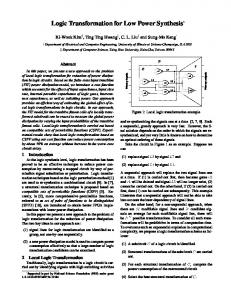
Example 1 Figure 1.(a) shows a network which repre-

sents the original speci cation. In general, a speci cation may be given in a high{level description language, but here for illustration purpose, we simply take the network in Figure 1.(a) as the initial speci cation. After applying logic transformation and optimization procedures [1, 2, 3] on the network in Figure 1.(a), the resulting network is shown in Figure 1.(c). Now suppose the speci cation in Figure 1.(a) has been slightly modi ed by changing p5 from an XOR gate to an AND gate, as shown in Figure 1.(b). After applying the same synthesis procedures as before, we obtain a network shown in Figure 1.(d). As we can see, although the change in speci cation arises from a local modi cation, general synthesis procedures do not localize such a change and the networks in Figure 1.(c) and Figure 1.(d) are quite dierent (i.e. the number of gates is changed from 10 to 9, and ve out of the nine gates have dierent fanins or fanouts). Another way to handle the speci cation change is to modify the network in Figure 1.(c) directly, so that we can obtain a network similar to Figure 1.(c), yet realizing the new speci cation in Figure 1.(b). Such manual EC technique, however, cannot be easily applied in this case. This is because after we have applied transformation and optimization procedures, the signal corresponding to gate p5 in Figure 1.(a) is no longer available in the optimized network Figure 1.(c). Therefore, although we know the change arises from the modi cation of p5 , it is dicult to tell in Figure 1.(c) where and how the modi cations should be done. On the other hand, a good synthesis procedure which considers engineering changes will be able to modify the network in Figure 1.(c) minimally, such that the resulting network is functionally equivalent to the speci cation in Figure 1.(b). In later sections, we will discuss such EC algorithms. By applying these algorithms on the network in Figure 1.(c), the network in Figure 1.(e) is obtained, diering from the network in Figure 1.(c) in that the gates, k0 ; k1 and k2, have been removed and a gate k3

y0

II. Terminology and previous work

y0

x1 x3 x4

x1 x3 x4 x1

x5

x1

y2

p5

x2

x5

p5

x2

x0

y2

x0 y1

y1

(b) a new specification.

(a) the original specification. x1

y0

y0

x3 x4

x1

k1

x2 x0

k0

k2

t p1

x3 x4

y2

y2 x5

x2 x0

x5

y1 y1 x1

(c) a circuit synthesized from the specification in (a).

(d) a circuit synthesized from the new specification in (b).

x1

y0

x3 x4 x2 x0

k3

t

y2

x5 y1 x1

(e) a circuit synthesized by applying EC algorithm.

Fig. 1. An example of the EC problem.

has been added. Note that the removal of gates is probably bene cial for layout and timing, and the change made here is local. 2

Note that changes made at high levels can potentially introduce large changes in the nal design. For example, suppose a design is described in terms of a nite{ state machine, and modi cations were made resulting in changes in the number of states and state transitions. Then, during synthesis, state encoding dierent from the original encoding may be used, potentially leading to a very dierent network. Therefore, it should not be expected that engineering changes can always be done with very few modi cations. In this paper, we will concentrate on the core problem of the engineering change, i.e., handling functional speci cation changes for combinational networks. Remainder of this paper is organized as follows. Section II provides appropriate background, de nitions and reviews related work. Section III, Section IV and Section V discusses our approach of logic synthesis for engineering change. Section VI summarizes the overall EC algorithm. Section VII shows the experimental results. Finally we give conclusions and discuss the plan for future work.

Let S o be the original speci cation and C o a corresponding synthesized logic network. Suppose S n is a new speci cation resulting from engineering changes. The goal of logic synthesis for engineering change is to synthesize a network C n such that it realizes S n and the structural dierences between C o and C n are minimized. In the remainder of the paper, we shall simply refer to S o (S n ) and C o (C n) as the old (new) speci cation and network, respectively. There have been several papers on logic synthesis algorithms for engineering change. In [4], C o and C n are synthesized independently from S o and S n , respectively, and then a post{processing step is performed to identify the correspondence between pins and gates of C o and C n. This method is eective when C o and C n are structurally similar, but this is often not the case with existing logic synthesis algorithms which tend to change substantially the structure of the networks. In [5], the idea was to leave the old network C o totally unchanged, and to rectify the speci cation changes by attaching pre{logic and post{logic networks to the primary inputs and outputs of C o . Boolean relation based algorithms were developed to derive the functions of the pre{ and post{logic. It has been shown that any new speci cation can be realized in this way if both pre{ and post{logic networks are allowed. In [6], the application of Boolean uni cation techniques to solve the same problem (i.e., derive the functions of the pre{ and post{ logic) were discussed. This approach is useful when changes are made at a later stage of the design process when it may be desirable to keep the old design unchanged. For example, it can be used to patch an existing layout for function changes, without going through the whole layout process again. However, the pre{ and post{logic added may still be too large to be useful, and it is not suitable in situations where the internal structure of the old network can be modi ed. In [7], a novel approach is proposed which explores the structural equivalence between the old and new speci cations, and the functional equivalence between the old speci cation and the existing synthesized network. Using these structural and functional equivalence, [7] establishes a mapping between the signals in the existing network and the ones in the new speci cation. Then, this mapping information is used to guide an ATPG{based logic substitution process. This method is computationally ecient. However, its eectiveness depends on the amount of the functional equivalence between the old speci cation and the existing synthesized network. In the last few years, there have been much work on the problem of error diagnosis [8, 9, 10, 11, 12]. The error diagnosis problem can be viewed as an engineering change problem if the appropriate networks are interpreted as follows. C o is supposed to implement the speci cation S n and contains an implementationerror such that it actually

implements S o and S o 6= S n . Therefore, the correct speci cation S n is now the new speci cation, and our goal is to modify C o into another network C n which implements S n correctly. In [8, 9, 10, 11], error correction techniques were proposed based on a single{error model which assumed that the structural dierence between C o and C n can be characterized as a single gate type change or a single wire mis{connection. The error diagnosis problem has a strong relationship to the EC problem. However, in EC problems, changes in speci cation can potentially result in diverse changes in a network, and it is often necessary to make multiple changes in the old network in order to realize a new speci cation. As a result, single{error model does not suce. An extension of single{error model for the EC problem is shown in [13] which modi es multiple signals sequentially in the following steps: 1) Identify all erroneous outputs, POerror . 2) Identify a single candidate signal which can rectify as many erroneous outputs as possible, and also derive the new function of this signal. 3) Synthesize the new function by utilizing existing logic of the old network. 4) Remove the corrected outputs from POerror . If POerror is not empty, then loop back to Step 2. To realize the new speci cation with minimal modi cations, the above process should identify as few signals as possible, and the synthesis procedures in Step 3 have to be powerful enough so that the new functions can be realized using as few gates as possible. In this paper, following the framework of [13], we develop a new algorithm which identi es multiple signals simultaneously for Step 2 based on the concept of coobservable domain. As a result, the new algorithm can search a larger solution space and the experimental results are competitive. III. Observable and co{observable domain

In the EC problem, given an existing network and a new speci cation, we are interested in modifying the network minimally to realize the new speci cation. It is the modi cation of internal signals' logical functions that allows the new speci cation can be realized. Therefore, we should have a way to detect and measure the eects of internal signals on the network's functionality. Based on the concept of observability don't care [1] and Boolean relation [14, 15, 16], we de ne observable domain for a single signal and co{observable domain for multiple signals, respectively. They completely characterize the eects of internal signals on the network's functionality. For simplicity, in the following Section A and Section B, we assume the existing network C o has a single output

realizing f(X) where X is the set of primary inputs. The extension to multiple outputs is discussed in Section C. f(X) is assumed to be dierent from the new speci cation f s (X) and the error minterm set is de ned as Ef (X) = f(X)  f s (X); where Ef (X) can be viewed as a set of minterms or a Boolean function. De nition 1 A set of signals t1 ;


; tk in the network C o

is a candidate location set if there exists a new function tni (X) for each ti , such that after substituting ti (X) (the original function of ti with respect to the primary inputs X ) by tni(X), f(X) is equal to f s (X).

A. Observable domain Given a signal ti , the observable domain (OD) of ti is de ned as follows: De nition 2 Let f t (X; ti) be a representation of f(X) by treating ti as an input. The observable domain of ti with respect to f is a set of minterms, where ODtf (X) = fX1 j f t (X1 ; ti) 6= 0 or 1; for X1 2 2X g: For a given minterm X1 in ODtf (X), when its applied to f t (X; ti ), it will make ti observable at the output. In other words, under the input minterm X1 , the value ti controls the value of f t . On the other hand, if X1 is not in ODtf (X), then the value of ti has no control on the value of f t (i.e., X1 is an observability don't care of the signal ti [1]). i

i

i

i

i

i

i

i

Example 2 Figure 2 shows a network with the out-

put function f(a; b; c). To compute the observable domain of the signal t1 , rst of all, f is re-expressed as f t1 (a; b; c; t1) = ab + t1 (b + c) by considering t1 as an extra input. Then, based on the above de nition, we can nd that among all the 8 dierent minterms, the minterms fabc; abcg make f t1 become 1, while the minterms fabc; abcg make f t1 become 0. As a result, ODt1 is fabc; abc; abc; abcg or we can express it more conveniently as ab + ac + bc. 2

Based on the notion of observable domain, we have the following sucient condition for a set of signals to be a candidate location set. Lemma 1 A set of signals, t1;


; tk , is a candidate location set, if

Ef (X) 

[k ODf (X):

i=1

ti

Proof. Given an error minterm in Ef (X), we can nd at least a ti such that if we switch ti (X)'s value for that minterm, then the output is recti ed for that error minterm. Since each error minterm can be recti ed independently, the lemma follows.

C. Handling multiple outputs Here, we show how to extend the de nition of OD and COD to multiple{output networks. Assume the network has outputs f1 ;


; fm , and the new speci cations are f1s ;


; fms . We construct a single output network Z(X) as follows:

t2

a

t1

f

b c

Fig. 2. Example of the observable domain and co{observable domain. The observable domain of the signal t1 is ab + ac + bc and the co{observable domain of signal t1 and t2 is a + b + c.

Z(X) =

_m f (X)  f s(X); i

i=1

i

where Z(X) is not equal to the zero function (otherwise the network has already implemented the new speci cation). Then, the problem of rectifying multiple outputs becomes the problem of rectifying a single output network B. Co-observable domain Z(X), where its new speci cation Z s (X) is the zero funcThe condition of Lemma 1 is sucient but not neces- tion. Note that here we are only allowed to modify the sary because it does not consider the interaction of mul- signals in the fanin cones of f1 ;


; fm . tiple signals. We introduce the concept of co-observable domain to handle such a case. Given two signals ti and tj , their co-observable domain (COD) is de ned as follows: IV. COD Computation and search of candidate location set

De nition 3 Let f t ;t (X; ti; tj ) be a representation of

In this section, given a signal ti or a set of signals f(X) by treating ti and tj as inputs. The co-observable t1 ;


; tk, we show how to compute ODt and CODt1 ; ;t domain of ti and tj with respect to f , is eciently based on BDD manipulations [17]. Then, we show how to use ODt eectively to guide the search for CODtf ;t (X) = f X1 j f t ;t (X1 ; ti; tj ) 6= 0 or 1; a candidate location set while using Theorem 1 to verify its candidacy. X for X1 2 2 g: A. COD Computation Since COD considers the interaction of signals, we have Since OD is a special case of COD, we only discuss the following lemma. how to compute COD. Given a set of signals t1;


; tk , rst construct BDDf , which is a BDD for f in term Lemma 2 Given two signals ti and tj , their COD is a we of X and t1;


; tk . Then we apply the consensus opersuper set of the sum of ODi and ODj , i.e., ator and smoothing operator on BDDf with respect to [ ODf (X)  CODf (X): the BDD variables t1 ;


; tk to obtain BDDfc and BDDfs ODtf (X) t t ;t separately. BDDfc contains all the minterms which make BDDf 1 and BDDfs contains all the minterms which Example 3 We use Figure 2 again to show the concept of make BDDf not equivalent to 0. Since COD is the set co{observable domain. To compute the co{observable do- of minterms which make BDDf not equivalent to 1 or 0, main of the signals t1 and t2 , rst of all, f is re-expressed the dierence between BDDfs and BDDfc is COD. The as f t1 ;t2 (a; b; c; t1; t2) = t2a +t1(b+c) by considering t1 ; t2 pseudo code for computing co-observable domain is as folas two extra inputs. Then, we nd that among all the 8 lows: dierent minterms, no minterms can make f t1 ;t2 become 1, while the minterm in fabcg makes f t1 ;t2 become 0. As COD(f; X; t1;


; tk ) a result, CODt1 ;t2 is a + b + c. 2 f BDDf = build bdd(f; X; t1 ;


; tk) We can also extend the de nition of co-observable doBDD cod = Smootht1; ;t (BDDf ) main to more than two signals. Using the concept of Consensust1 ; ;t (BDDf ) COD, we have the following necessary and sucient conreturn(BDD ) cod dition for a set of signals to be a candidate location set. g. Theorem 1 A set of signals t1;


; tk is a candidate loB. Search of a candidate location set cation set, i Since there are huge combinations of signals, we have Ef (X)  CODtf1; ;t (X): to develop heuristics to guide the search for a candidate i

j

i

i

i

j

i

i

j

j

i

j






k











k

k






k

search candidate location set(Ef ; k)

f

g

compute OD foreach signal() T =; C = sorted candidate signals by OD coverage loop f t = rst candidate(C) if (t is not dominated by sigals in T) T = minimal dominating set(T + ftg) COD = compute COD(T) end C = C ftg if (Ef  COD) return(T) g until ( size of(T ) > k) or (C is ;) return(;)

Fig. 3. The pseudo code for searching a candidate location set guided by observable domain. The parameter k is the size constraint of T .

location set. This can also be considered as a multiple{ error diagnosis problem [12]. In our approach, we utilize the information extracted from OD to guide the search. Moreover, to avoid redundant computation, topological information can be utilized. For example, given a set of signals t1;


; tk , if CODt1; ;t is not a candidate location set, then any combinations of signals in the fanin cones of t1;


; tk are not either. The overall searching procedure is shown in Figure 3. First, the observable domain of each signal ti (ODt ) is computed and stored. Then the signals are sorted according to their coverage of Ef , i.e., the number of minterms in ODt ^ Ef . After that, the algorithm sequentially adds one signal to the set T until its COD satis es Theorem 1. Theoretically, without size constraint, given enough time, the algorithm should be able to nd a candidate location set T which satis ed Theorem 1, but for practical purpose, we set a size constraint k as shown in Figure 3 to avoid the memory explosion due to BDD operations. Note that, by setting the size constraint to 1, the algorithm proposed in [13] becomes a special case of this new approach.




k

i

i

the new functions of these signals. After the new functions of these signals are decided, we apply the substitution methods [13] to realize these new functions by utilizing the existing gates of the network. Like many problems in logic minimization, it's dicult to formulate an exact cost function for deciding what new functions the signals ti 's should have. Here, the ultimate goal is to make the new functions easier to be synthesized by utilizing the existing gates of the network. We developed two heuristic procedures to decide the on{set and o{set of tni (X). Both of them are designed such that the synthesis procedures (Step 3 in Section II) can take advantage of the freedom of Boolean relation. These two heuristics are 1) minimize the sum of the numbers of minterms changed between ti (X)'s and tni(X)'s. 2) minimize the number of tni(X)'s BDD nodes. A. Freedom of choosing new functions for a candidate location set As discussed in Section C, we assume the multiple{ output network and the new speci cation have been merged into a single{output network Z(X). The on{set of Z(X) denotes the error minterms, while Z s (X) is the zero function. The freedom for determining the on{set and o{set of tni is completely characterized by the following characteristic function which represents a Boolean relation among tn1 ;


; tnk: K = Z t1 ; ;t (X; tn1 ;


; tnk) = 0:




k

In other words, any combinations of tni(X)'s are legal if after substituting ti (X)'s by tni(X)'s, the resulting Z t1 ; ;t is the zero function. In the following, for simplicity, we use Z to denote Z t1 ; ;t .









k

k

B. Minimize the dierence between ti (X) and tni(X) This heuristic nds a realization such that the dierence between ti (X) and tni (X) is minimized. We use the number of minterms in ti (X)  tni (X) to measure the difference. The problem can be formally stated as follows: given a Boolean relation of t1;


; tk , Z(X; t1 ;


; tk ) = 0; nd a realization tni (X) for each P ti such that the total number of dierent minterms, ki=1 kti(X)  tni (X)k; is minimized. V. Synthesizing functions for signals in a We can derive an optimal solution by dynamic procandidate location set gramming to traverse the BDD graph once. In this forGiven a set of signals t1 ;


; tk , if its COD covers all the mulation, given a minterm, we need to know what the old error minterms, there exists a new function tni(X) for each values of ti 's are. The following characteristic function, ti, such that by replacing each ti by tni (X) simultaneously, Yk all the error minterms can be corrected. In this section, we P1 = (toi  ti (X)); discuss the freedom we have and the methods for deciding i=1

have to modify the characteristic function K by applying bdd compose operator [1] which substitutes the BDD variable ti of K by function tni (X). The algorithm is as follows:

N t t

n

i o

i

MINIMIZE BDD SIZE(K)

f

N 00 N 01 N 10 N 11

Fig. 4. Example of combining two BDD variables tni and toi into one super BDD variable with 4 sons.

captures these information in a BDD formula, where toi 's represent the old value of ti 's. We then construct the following BDD, P = Z(X; tn1 ;


; tnk) ^ P1(X; to1;


; tok );

z }| { z }| { z }| { < tn < to < tn < to <


< tn < to : 1

1

2

2

k

i

i

i

g.

i

i






k

i

i






k

i

VI. The overall EC algorithm

with BDD variable ordering as follows: x1 <


< xn

for i = 1 to k Kt = cofactort (K) Kt = cofactort (K) on = Ct +1; ;t (Kt ) off = Ct +1; ;t (Kt ) tni(X) = bdd minimize(on; off) K = bdd compose(K; ti; tni(X)) end

k

There are two BDD variables tni and toi associated with each ti . In the BDD P , a path X1 ; tn1 ; to1;


; tnk; tok which leads to 1{terminal node of BDD, represents what the old value (toi ) of ti is and what legal value (tni ) for ti can be for the given minterm X1 . To nd an optimal solution, we virtually combine two BDD variables tni and toi into one super BDD variable (with 4 sons) as shown in Figure 4 and traverse the BDD P in a depth{ rst manner for all the BDD nodes of P with indices greater than or equal to tn1 . During the BDD traversal, the cost function for a BDD node is computed as as follows: Cost(N) = MINf Cost(N00 ); Cost(N01) + 1; Cost(N10 ) + 1; Cost(N11) g; where N is a BDD node and N00; N01; N10; N11 are the four sons of the BDD node N. The cost of the 1{terminal and 0{terminal nodes are zero and in nite, respectively. Using this cost function in the BDD traversal, we can optimally decide the values of tni 's for each minterm implicitly . C. Minimize the number of BDD nodes of tni(X)'s The second heuristic is to nd a realization of tni (X)'s, such that the number of BDD nodes is minimized. As a result, the obtained functions might be easier to implement. Since it is dicult to nd a global minimum solution, we sequentially extract the maximal freedom allowed to implement each tni (X)'s and then apply the bdd minimize algorithm [18, 19] to minimize the number of BDD nodes. After the new function tni (X) for ti has been decided, we

In Section IV, we showed the algorithm to nd a candidate location set T , where there exists a new function tni (X) for each signal ti in T, such that the result of substituting ti by tni (X) in the existing network will realize the new speci cation. In Section V, we discussed two dierent heuristics to decide the new functions of ti 's. Thus, the remaining work is to realize these new functions by utilizing the existing gates of the network as much as possible. We apply the direct substitution and indirect substitution methods proposed in [13] for this purpose. We brie y describe these substitution methods here. For more details, please refer to [20, 2, 3, 13]. A connection conni = (Si ; Di ) is a signal, where Si and Di are its source and destination gates. A connection conn2 = (S2 ; D2 ) is called substitutable by another connection conn1 = (S1 ; D1 ) if the functionality of the network remains unchanged after adding conn1 and removing conn2. In the case where D1 is equal to D2 , conn2 is called directly substitutable by conn1. The exact requirement of conn2 being directly substitutable by conn1 are shown in [20, 21]. In the case where D1 is dierent from D2 , conn2 is called indirectly substitutable by conn1. Based on the concept of indirect substitution, an ATPG{based approach is shown in [2, 3] for logic optimization. To apply these substitution methods for our purpose, we rst synthesize a network C T for the new functions tni 's based on their BDD representations (independent from the existing network). Then, the indirect and direct substitution algorithms are used iteratively to utilize the signals (or gates) in the existing network C o to replace the signals in C T . The overall EC algorithm is shown in Figure 5, where POerror (POcorrect ) denotes the set of outputs which are dierent (equivalent) in the old and new speci cations. Before calling the EC algorithm, an BDD{based veri cation tool [1] is used to nd POerror and POcorrect. Due to

topology between S o and C o are quite dierent also. To obtain S n , we randomly modi ed S o by changing EC(C o ; S n ; POerror ; POcorrect; k) the function of internal gates. For a complex gate (repref sented as a SOP form in BLIF format [1]), we arbitrarily Ef= compute error minterm set(C o ; S n ; POerror ) modi ed its cubes. For a simple gate, say an AND gate, T = search candidate location set(Ef ; k) we changed it to an OR gate, etc. The fth column of Figif T 6= ; ure 6 shows the number of such changes and the number EC COD synthesize(C o ; T) of primary outputs aected. append POerror to POcorrect Then, given C o and S n , we applied the EC algorithms else to generate C n. We test both heuristics described in SecfPO1error ; PO2error g partition(POerror ) tion V with the constraint 5 on the size of the candidate EC(C o ; S n ; PO1error ; POcorrect) location set. The results for the algorithms in Section EC(C o ; S n ; PO2error ; POcorrect) V.B and Section V.C are shown in the columns labeled end M1 and M2, respectively. For comparison, the results g from [13] are listed in the column labeled M0. We report the number of added gates (A), removed gates (R) EC COD synthesize(C o ; T) and computation time (seconds). They could be used to f measure the quality of the EC algorithms. tni 's = decide functions from Boolean relation(C o ; T) The columns labeled P shows the results of recursively replace ti by tni in C o partitioning erroneous outputs. For example, (3; 1; 2) loop f means that during searching for a candidate location set, perform indirect substitution(C o ) the 6 erroneous outputs in POerror were partitioned into 3 perform direct substitution(C o ) sub{groups. Each of them was recti ed separately. As exg until (no further improvement) pected, M1 and M2 partition POerror into fewer number g of sub{groups. This is because they explore the chances of modifying multiple signals simultaneously. In terms of the EC quality, for the example b9 , M1 and Fig. 5. The pseudo code of EC algorithm. M2 perform better than M0, while for x2 , the results from M0 is better. Although M0 is a special case of M1 and M2, on the average, the results for three dierent the imposed size constraint k, the algorithm might fail to heuristics are quite competitive. This is probably because nd a candidate location set to rectify all the outputs in of the inaccuracy of the cost function. In other words, the POerror . If this happens, POerror is split into two sub{ nal results of EC algorithms also depend on the synthesis set PO1error and PO2error , and the EC algorithm recti es methods used to synthesize the new functions. During the them separately. process of determining those new functions, it is dicult to use a cost function which accurately represents the nal synthesis results. VII. The Experiment

In this section, we show the experimental results of applying the EC algorithm described in the previous section. Several combinational benchmark circuits from MCNC91 and one industrial example (SrCr) from Fujitsu are included in our test suite. The circuit SrCr (part of an ATM router chip) originally was given in VHDL by the designer and, later on, the speci cation was modi ed by creating a new signal. It was a hierarchical design and contained ip{ ops. For our experiment, we attened the design and extracted the combinational portion of the circuit. For MCNC91 benchmarks, it was assumed that each of them represents the original speci cation S o . To obtain C o , we optimized S o by running script.rugged script and then performed technology decomposition (tech decomp {a 4 {o 4) in SIS [1]. The numbers of gates in S o and C o are shown in the third and fourth column of Figure 6 respectively. Beside the dierence in the number of gates, the networks'

VIII. Conclusions and Future Work

In this paper, synthesis algorithms for the engineering change problem are described. To realize changes of the

speci cation, we developed algorithms to modify the existing synthesized network minimally such that substantial portion of engineering eort can be preserved. Our EC algorithm can be divided into two steps. The rst step identi es multiple candidate signals, such that replacing them simultaneously with appropriate new functions can rectify the dierence between the old and new speci cations. The next step synthesizes these new functions by utilizing gates of the existing network. Deciding which signals to change is a major problem in all minimization algorithms which try to change multiple signals concurrently. In our approach, this problem is solved by using the concepts of observable and coobservable domains to guide the search. Currently, mul-

tiple signals identi cation and synthesis of new functions [12] A. Kuehlmann, D.I. Cheng, A. Srinivasan and are performed independently. Future improvement will D.P. LaPotin, \Error diagnosis for transistor-level consider new algorithms which integrate these two steps veri cation," ACM/IEEE Design Automation Conclosely such that we can obtain more accurate estimate of ference, pp. 218{224, 1994. the nal changes in the EC algorithm. [13] C.C. Lin, K.C. Chen, S.H. Chang, M. Marek-Sadowska and K.T. Cheng, \Logic synthesis for engineering Acknowledgements change," ACM/IEEE Design Automation ConferThis work was supported in part by the National Science, 1995. ence Foundation under Grant MIP 9419119 and in part [14] E. Cerny and M. A. Marin, \An approach to uni ed by the California MICRO program. methodology of combinational switching circuits," IEEE Trans. on Computers, pp. 745{756, 1977. References [15] R.K. Brayton and F. Somenzi, \An exact minimizer [1] \SIS: A system for sequential circuit synthesis," for boolean relations," ICCAD, pp. 316{319, 1989. Report M92/41, University of California, Berkeley, [16] Y. Kukimoto and M. Fujita, \Recti cation method 1992. for lookup{table type FPGA's," ICCAD, pp. 54{61, 1992. [2] K.T. Cheng and L.A. Entrena, \Multi-level logic optimization by redundancy addition and removal," [17] R. E. Bryant, \Graph{based algorithms for boolean Proc. European Conference on Design Automation, function manipulation," IEEE Trans. Computers, pp. 373{377, 1993. vol. C-35, pp. 667{691, 1986. [3] S.C. Chang and M. Marek-Sadowska, \Perturb and [18] S.C. Chang, D.I. Cheng and M. Marek-Sadowska, simplify: multi-level boolean network optimizer," IC\BDD representation of incompletely speci ed funcCAD, 1994. tions," EDAC, pp. 620{624, 1994. [4] T. Shinsha, T. Kubo, Y. Sakataya and K. Ishihara, [19] \Incremental logic synthesis through gate logic strucT.R. Shiple, R. Hojati, A.L. Sangiovanni-Vincentelli ture identi cation," ACM/IEEE Design Automation and R. K. Brayton, \Heuristic minimization of bdds Conference, pp. 391{397, 1986. using don't cares," ACM/IEEE Design Automation Conference, pp. 225{231, 1994. [5] Y. Watanabe and R.K. Brayton, \Incremental synthesis for engineering changes," ICCAD, pp. 40{43, [20] S. Muroga, Y. Kambayashi, H.C. Lai and 1991. J.N. Culliney, \The Transduction method { design of logic networks based on permissible functions," [6] M. Fujita, Y. Tamiya, Y. Kukimoto and K.C. Chen, IEEE Trans. on Computers, pp. 1404{1424, 1989. \Application of boolean uni cation to combinational logic synthesis," ICCAD, pp. 510{513, 1991. [21] D. Brand, \Veri cation of large synthesized designs," ICCAD, pp. 534{537, 1993. [7] D. Brand, A. Drumm, S. Kundu and P. Narain, \Incremental synthesis," ICCAD, 1994. [8] J. C. Madre, O. Coudert, J.P. Billon, \Automating the diagnosis and the recti cation of design errors with PRIAM," ICCAD, 1989. [9] H.T. Liaw, J.H. Tsaih and C.S. Lin, \Ecient automatic diagnosis of digital circuits," ICCAD, pp. 464{ 467, 1990. [10] P.Y. Chung, Y.M Wang and I.N. Hajj, \Diagnosis and correction of logic design errors in digital circuits," ACM/IEEE Design Automation Conference, pp. 503{508, 1993. [11] I. Pomeranz and S. M. Reddy, \On error correction in macro-based circuits," ICCAD, pp. 568{575, 1994.

So C o 4 28

z4ml

I/O 7=4

b9

41=21 117 89

frg1

28=3

3

115

count 35=16 47

79

x1

51=35 28 207

x2

10=7

12

25

C880 60=26 357 261 SrCr 85=82 272 339

EC Results of EC algorithms Sn M0 M1 changes; POerror P A,R time P A,R time 1; 1 1 4; 3 7 1 4; 3 4 2; 2 1; 1 6; 3 10 2 5; 1 12 3; 3 1; 1; 1 7; 3 30 1; 2 6; 1 23 4; 4 1; 1; 1; 1 6; 0 24 1; 1; 2 5; 0 16 1; 2 1; 1 6; 2 4 2 3; 2 1 2; 3 1; 1; 1 6; 3 14 3 4; 3 5 3; 4 1; 1; 1; 1 7; 3 33 3; 1 4; 3 20 4; 6 1; 1; 1; 1; 2 10; 7 123 3; 1; 2 8; 7 71 1; 1 1 3; 0 67 1 3; 0 120 2; 2 1; 1 4; 1 74 2 6; 2 149 3; 3 1; 1; 1 7; 2 71 1; 2 6; 2 170 4; 3 1; 1; 1 7; 5 74 1; 2 7; 3 161 1; 1 1 2; 0 4 1 2; 0 3 2; 2 1; 1 4; 1 8 2 4; 2 5 3; 2 1; 1 7; 2 10 2 6; 4 8 4; 3 1; 1; 1 8; 4 34 1; 2 7; 5 23 1; 1 1 4; 1 25 1 4; 1 17 2; 2 1; 1 5; 2 31 1; 1 5; 2 22 3; 3 1; 1; 1 7; 3 79 1; 1; 1 7; 3 60 4; 4 1; 1; 1; 1 8; 4 104 1; 1; 1; 1 8; 4 77 1; 1 1 1; 1 1 1 1; 1 0:7 2; 2 1; 1 1; 3 2 2 3; 5 2 3; 3 1; 1; 1 5; 4 13 1; 1; 1 12; 7 15 4; 4 1; 1; 1; 1 3; 8 7 2; 1; 1 3; 8 7 1; 1 1 1; 1 69 1 1; 1 102 2; 2 1; 1 1; 12 72 1; 1 1; 12 120 3; 3 1; 1; 1 2; 13 285 1; 1; 1 2; 13 426 4; 4 1; 1; 1; 1 2; 12 251 1; 1; 1; 1 2; 12 437 2; 1 1 20; 5 1471 1 20; 5 1471

Fig. 6. The experimental results of the EC algorithms

P 1 2 1; 2 1; 1; 2 2 3 3; 1 3; 1; 2 1 2 1; 2 1; 2 1 2 2 1; 2 1 1; 1 1; 1; 1 1; 1; 1; 1 1 2 1; 1; 1 2; 1; 1 1 1; 1 1; 1; 1 1; 1; 1; 1 1

M2 A,R time 4; 3 4 10; 5 5 9; 1 23 5; 0 17 3; 2 1:7 3; 3 2 4; 3 20 7; 7 70 3; 0 104 6; 1 151 7; 3 165 6; 5 161 2; 0 3 4; 2 3 5; 3 4 6; 4 23 4; 1 16 5; 2 23 7; 3 63 8; 4 79 1; 1 0:7 2; 5 1 12; 7 16 2; 8 6 1; 1 106 1; 12 124 2; 13 442 2; 12 447 20; 5 1471