Low-Dose CT with a Residual Encoder-Decoder Convolutional - arXiv

Low-Dose CT with a Residual Encoder-Decoder Convolutional Neural Network (RED-CNN) Hu Chen1, Yi Zhang1,*, Mannudeep K. Kalra2, Feng Lin1, Peixi Liao3, Jiliu Zhou1, and Ge Wang4 1. College of Computer Science, Sichuan University, Chengdu 610065, China 2. Department of Radiology, Massachusetts General Hospital, Boston, MA 02114, USA 3. Department of Scientific Research and Education, The Sixth People’s Hospital of Chengdu, Chengdu 610065, China 4. Department of Biomedical Engineering, Rensselaer Polytechnic Institute, Troy, NY 12180 USA * Corresponding author: [email protected] Abstract—Given the potential X-ray radiation risk to the patient, low-dose CT has attracted a considerable interest in the

medical imaging field. The current main stream low-dose CT methods include vendor-specific sinogram domain filtration and iterative reconstruction, but they need to access original raw data whose formats are not transparent to most users. Due to the difficulty of modeling the statistical characteristics in the image domain, the existing methods for directly processing reconstructed images cannot eliminate image noise very well while keeping structural details. Inspired by the idea of deep learning, here we combine the autoencoder, the deconvolution network, and shortcut connections into the residual encoder-decoder convolutional neural network (RED-CNN) for low-dose CT imaging. After patch-based training, the proposed RED-CNN achieves a competitive performance relative to the-state-of-art methods in both simulated and clinical cases. Especially, our method has been favorably evaluated in terms of noise suppression, structural preservation and lesion detection. Index Terms—Low-dose CT, deep learning, auto-encoder, convolutional, deconvolutional, residual neural network.

I. INTRODUCTION X-ray computed tomography (CT) has been widely utilized in clinical, industrial and other applications. Due to increasing use of CT, concerns have been expressed on increasing contribution to overall radiation dose to the population. The research interest has been strong in medical CT dose reduction under the well-known guiding principle of ALARA (as low as reasonably achievable) [1]. The most common way to lower the radiation dose is to reduce the X-ray flux by decreasing the operating current and shortening the exposure time of an X-ray tube. In general, the weaker the X-ray flux, the noisier a reconstructed CT image, which can degrade the diagnostic performance. To address this inherent physical problem, many algorithms were designed to improve the image quality for low-dose CT (LDCT). These algorithms can be generally categorized into three categories: (a) sinogram domain filtration, (2) iterative reconstruction, and (3) image processing. Sinogram filtering techniques can perform on either raw data or log-transformed data before an image reconstruction algorithm, such as filtered backprojection (FBP), is applied. The main advantage of these methods is that the noise characteristic has been well characterized in the sinogram domain. Typical methods include structural adaptive filtering [2], bilateral filtering [3], and penalized weighted least-squares (PWLS) algorithms [4]. However, the sinogram filtering methods often suffer from spatial resolution loss when edges in the sinogram domain are not preserved. Over the past decade, iterative reconstruction (IR) algorithms have attracted much attention in the field of LDCT. This approach combines the statistical properties of data in the sinogram domain, prior information in the image domain, and even parameters of the imaging system into one unified objective function. With compressive sensing (CS) [5], several image priors were formulated

as sparse transforms to deal with the low-dose, few-view, limited-angle and interior CT issues, such as total variation (TV) and its variants [6-9], nonlocal means (NLM) [10-12], dictionary learning [13], low-rank [14], and other techniques. Model based iterative reconstruction (MBIR) modeled the physical acquisition processes and has been equipped into some current CT scanners [15]. Although IR methods obtained exciting results, there are two weaknesses. First, on most newer MDCT scanners, IR techniques have replaced FBP based image reconstruction techniques for enabling radiation dose reduction. However, these IR techniques are vendor-specific since the details of the scanner geometry and correction steps are not available to non-vendor personnel. Second, there are substantial computational overhead expenses and costs associated with most IR techniques. Fully model based iterative reconstruction techniques have greater radiation dose reduction potential but slow reconstruction speed and changes in image appearance limit their applications for routine CT protocols. An alternative for LDCT is post-processing of reconstructed images, which does not rely on raw data. These techniques can be directly applied on LDCT images, and integrated into any CT system. In [16], NLM was introduced to take advantage of the feature similarity within a large neighborhood in a reconstructed image. Inspired by the theory of sparse representation, dictionary learning [17] was adapted for LDCT, and resulted in substantially improved image quality of LDCT of the abdomen [18]. Meanwhile, Block-matching 3D (BM3D) was proved efficient for various X-ray imaging tasks [19-21]. In contradiction to the other two kinds of methods, an accurate distribution of image noise cannot be statistically determined, which prevents users from achieving the optimal tradeoff between structure preservation and noise supersession. Recently, deep learning (DL) has generated an overwhelming enthusiasm in several imaging applications, ranging from lowlevel to high-level tasks from image denoising, deblurring and super resolution to segmentation, detection and recognition [22]. It simulates the information processing procedure by human, and can efficiently learn high-level features from pixel data through a hierarchical network framework [23]. Several DL algorithms have been proposed for image denoising using different network models [24-30]. As the autoencoder (AE) has a great potential for image denoising, stacked sparse denoising autoencoder (SSDA) and its variant were introduced [24, 26]. Convolutional neural networks are powerful tools for feature extraction and have been applied for image denoising, deblurring and super resolution [27-29]. Burger et al. [30] analyzed the performance of multi-layer perception (MLP) to image patches and obtained competitive results to the state-of-the-art methods. Previous studies have applied DL for image analysis, such as image segmentation [31, 32], organ classification [33] and nuclei detection [34], but there are few reports on tomographic imaging topics. For example, Wang et al. incorporated a DL-based regularization term into a fast MRI reconstruction framework [35]. Chen et al. presented preliminary results with a light-weight CNN-based framework for LDCT imaging [36]. A deeper version using wavelet transform as inputs was presented last year [37], which won the second place in the “2016 NIH-AAPM-Mayo Clinic Low Dose CT Grand Challenge." Wurfl et al. mapped the filtered back-projection (FBP) workflow to a deep CNN architecture and reduced the reconstruction error by a factor of two in the case of limited-angle tomography [38]. Also, Wang shared his perspective on machine learning to have a major impact on tomographic reconstruction [39]. Despite the interesting results with CNN for LDCT, the potential of deep CNN has not been fully realized. Although some studies with CNN involved construction of deeper networks [40, 41], most image denoising models had limited layers (usually 2~3 layers) since image denoising is considered as a “low-level” task for suppressing noise and artifacts while preserving structural details instead of extracting features. This is in clear contrast to high-level tasks such as recognition or detection, in which pooling and other operations are widely used to bypass many image details. We incorporated a deconvolution network [42] and shortcut connections [40, 41] into a CNN model, which is referred to as a residual encoder-decoder convolutional neural network (RED-CNN). In the second section, the proposed network architecture is described. The third section deals with experimental evaluation and validation of the proposed model. In the final section, relevant

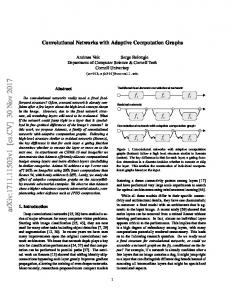
Fig.1. Overall architecture of our proposed RED-CNN network.

issues are discussed, and the conclusion is drawn. II. METHODS A. Noise Reduction Model Our image domain processing starts with a straightforward reconstruction from a low-dose scan, and the image denoising problem is restricted within the image domain [36]. Since the DL-based methods are independent to the statistical distribution of image noise, the LDCT problem can be simplified to the following one. Assuming that X  R mn

is a LDCT image and

Y  R m n

is a corresponding normal dose CT (NDCT) image, the relationship between them can be formulated as X   (Y)

(1)

where  : R mn  R mn denotes the complex degradation process involving quantum noise and other factors. Then, the problem can be transformed to seek a function f : arg min || f ( X)  Y ||22

(2)

f

where f is regarded as the optimal approximation of

 1 , and can be estimated using DL techniques.

B. Residual Autoencoder Network AE was originally developed for unsupervised feature learning with noisy inputs, which is also suitable for image restoration. In this context, CNN also demonstrated an excellent performance. However, due to its multiple down-sampling operations, some image details can be missed by CNN. For LDCT, here we propose a residual network combining AE and CNN. Rather than adopting fully connected layers for encoding and decoding in stacked autoencoder networks, we use both convolutional and deconvolutional layers in symmetry. Furthermore, different from the typical encoder-decoder structure, residual learning [42] with shortcuts is included to facilitate the operations of the convolutional and corresponding deconvolutional layers. The overall architecture of the proposed network is shown in Fig. 1. This network has total 10 layers, including 5 convolutional and 5 deconvolutional layers symmetrically arranged. Shortcuts are added into the network. Each layer except for the last one is followed by rectified linear units (ReLU) [43]. The details about the network are described as follows. 1) Patches extraction DL-based methods need a huge number of samples. This requirement cannot always be met in practice, especially in clinical imaging practice. In this study, we propose to use patches from overlapping regions in the images. This strategy has been found to be effective and efficient, because the perceptual differences of local regions can be detected, and the number of samples are significantly boosted [24, 27, 28]. In our experiments, we extracted patches from LDCT and corresponding NDCT images with a fixed size from the simulated and Mayo Contest database.

2) Stacked encoders (Feature extraction) Unlike traditional stacked AE networks, we use a chain of fully-connected convolutional layers as the stacked encoders. The features are extracted from low-level to high-level step by step in order to preserve primary components and essential information in the extracted patches. Moreover, since the pooling layer (down-sampling) after a convolutional layer may discard important structural details, it is abandoned in our encoder. As a result, there are only two types of layers in our encoder: convolutional layers and ReLU units, and the stacked encoders Cei ( xi ) can be formulated as Cei ( xi )  ReLU( Wi  xi  bi ) i  0,1..., N ,

where N is the number of convolutional layers, Wi and convolution operator,

(3)

b i denote the weights and biases respectively,  represents the

x0 is the extracted patch from the input images, and xi (i  0) is the extracted features from the previous

layers. ReLU( x)  max(0, x) is the activation function. After the stacked encoders, the image patches are transformed into a feature space, and the output is a feature vector

x N whose size is l N .

3) Stacked decoders (Image reconstruction) Although the pooling operation is removed, a serial of convolutions will still down-sample the input signals. Inspired by the recent results on semantic segmentation [44, 45], deconvolutional layers are integrated into our model to play the role of upsampling, which can be seen as image reconstruction from extracted features. We also adopt a chain of fully-connected deconvolutional layers to form the stacked decoders for image reconstruction. Since the encoders and decoders should appear in pair, the convolutional and deconvolutional layers are symmetric in the proposed network. Clearly, convolution is a down-sample process, while deconvolution is an up-sample progress. To ensure the input and output of the network match exactly, the convolutional and deconvolutional layers must have equal kernel sizes. Note that the data flow of convolutional and deconvolutional layers in our framework follows the rule of “FILO” (First In Last Out). As demonstrated in Fig. 1, the first convolution layer corresponds to the last deconvolutional layer, the last convolution layer corresponds to the first deconvolutional layer, and so on. In other words, this architecture is featured by the symmetry of paired convolution and deconvolution layers. There are two types of layers in our decoder network: deconvolution and ReLU. Thus, the stacked decoders Ddi (y i ) can be formulated as: Ddi (y i )  ReLU( Wi'

where N is the number of deconvolutional layers,

y i  bi' ) i  0,1..., N ,

Wi' and b i' denote the weights and biases respectively,

(4) represents

the deconvolutional operator, y N  x is the output feature vector after stacked encoding, y i ( N  i  0) is the reconstructed feature vector from the previous deconvolutional layer, and y 0

is the reconstructed patch. After stacked decoding, image patches

are reconstructed from features, and can be assembled to reconstruct a denoised image. 4) Residual compensation Different from the prior art methods [24, 25], convolution will eliminate some image details. Although the deconvolutional layers can recover some of the details, when the network goes deeper this inverse problem becomes more ill-posed, and the accumulated loss could be quite unsatisfactory for image reconstruction. Indeed, at the stage of optimization, when the network depth increases the gradient diffusion could make the network difficult to train. To address the above issue, inspired by deep residual learning [40, 46] we introduce a residual compensation mechanism into the proposed network. Instead of mapping the input to the output solely by the stacked layers, we adopt a residual mapping, as shown in Fig. 2. Defining the input as I and the output as O , the residual mapping can be denoted as F ( I )  O  I , and we

Fig.2. Shortcut: residual compensation structure

use stacked layers to fit this mapping. Once the residual mapping is built, we can reconstruct the original mapping as R( I )  O  F ( I )  I . Consequently, we transform the direct mapping problem to a residual mapping problem. There are two

benefits associated with this architecture. First, it is easier to optimize the residual mapping than optimizing the direct mapping. In other words, it helps avoid the gradient vanishing during training when the network is deep. For example, it would be much easier to train an identity mapping network by pushing the residual to zero than fitting an identity mapping directly. Second, since only the residual is processed by the convolutional and deconvolutional layers, much information and details can be preserved in the output of the deconvolutional layers, which can significantly enhance the LDCT imaging performance. 5) Training The proposed network is an end-to-end mapping from low-dose CT images to normal-dose images. Once the network is configured, the set of parameters, ={Wi ,bi ,Wi' , b i' } of the convolutional and deconvolutional layers should be estimated to build the mapping function M . The estimation can be achieved by minimizing the loss F ( D; ) between the estimated CT images and the reference NDCT images X . Given a set of paired train patches P ={(X1 ,Y1 ),(X 2 ,Y2 ),

Yi  denote NDCT and LDCT image patches respectively, and

, (X K ,YK )} where

Xi 

and

is the total number of training samples. The mean squared error

(MSE) is utilized as the loss function: F ( D; ) 

1 N

N

 i 1

2

X i  M (Yi ) .

(5)

In this study, the loss function was optimized by Adam [47]. III. EXPERIMENAL DESIGN AND RESULTS A. Data Sources 1) Simulated data The normal dose dataset included 7015 normal-dose CT images of 256×256 pixels per image from 165 patients downloaded from National Biomedical Imaging Archive (NBIA). Different parts of the human body were included for diversity. Some typical images are in Fig. 3. The corresponding dataset of LDCT images was produced by adding Poisson noise into the sinograms simulated from the normal-dose images. The noise level was controlled by the blank scan factor

which was set to

photons

in the initial studies. In our simulation, Siddon’s ray-driven method [48] was used to generate the projection data in fan-beam geometry. The source-to-rotation center distance was 40 cm while the detector-to-rotation center was 40 cm. The image region

Fig.3. Examples from our normal-dose CT image dataset.

was 20 cm ×20 cm. The detector width was 41.3 cm containing 512 detector elements. There were 1024 sampling angles uniformly distributed over a full scan. Since direct processing of the entire CT image is intractable, RED-CNN was applied to image patches. Our method benefits from the patch extraction since patch-based processing represents the local details required for optimal denoising and the number of samples were greatly increased for the training purpose. Deep learning methods require a large amount of training samples, but collecting medical images is usually limited by the complicated formalities addressing multiple factors such as the patient’s privacy. In the training step, 200 normal-dose and corresponding simulated low-dose images were randomly selected as the training set. Also, 100 image pairs were randomly selected as the testing set. Images from the patients in the training set were not in the testing set. 2) Clinial data To evaluate the clinical performance of RED-CNN, a real clinical dataset was used, which was authorized by Mayo Clinics for “The 2016 NIH-AAPM-Mayo Clinic Low Dose CT Grand Challenge”. The training set contained 3643 full and quarter dose 512×512 CT images from 10 patients [37]. The network was trained by 1mm thickness images while 3mm thickness quarter dose images were regarded as the testing set, and 3mm thickness full dose images as the standard of reference. For fairness, crossvalidation was utilized in the testing phase. While testing on CT images from each patient, the images from the other 9 patients were involved in the training phase. 3) Parameter selection The patch size  was set to 55×55 with the sliding interval of 4 pixels. After the patch extraction, the number of training patch pairs reached 106. Furthermore, three kinds of transformation operations, including rotation (by 45 degrees), flipping (vertical and horizontal) and scaling (scale factors were 2 and 0.5), were used for data augmentation. In our experiments, we evaluated several parameter combinations and finalized the parameter settings as follows. The network was trained with Caffe. The base learning rate was set to 10-4, and slowly decreased down to 10-5. The convolution and deconvolution kernels were initialized with random Gaussian distributions with zero mean and standard deviation 0.01. The kernel size of all layers was set to 5×5. All the experiments were performed with MATLAB 2015b on a PC (Intel i7 6700K CPU and 16 GB RAM). The training stage is time-consuming for

Fig. 4. Two representative slices from the testing set: (a) Chest, and (b) abdomen CT images.

Fig. 5. Results from the chest image for comparison. (a) LDCT, (b) TV-POCS, (c) K-SVD, (d) BM3D, (e) WaveNet, and (f) RED-CNN.

traditional CPU implementation. A common way for acceleration is to work in a parallel manner. In our work, the training of REDCNN was performed on a graphic processing unit card (GTX 1080). Although the training was done on patches, the proposed network can perform on images of arbitrary sizes. All the testing images were simply fed into the network, without decomposition. The three metrics, including the root mean square error (RMSE), peak signal to noise ratio (PSNR) and structural similarity index measure (SSIM), were chosen for quantitative assessment of image quality. Four different state-of-the-art methods were compared against our RED-CNN, including TV-POCS [6], K-SVD [18], BM3D [20] and WaveNet [37]. Dictionary learning and BM3D are two most popular image domain based denoising methods already applied for LDCT. ASD-POCS is a widely used iterative reconstruction method under the TV regularization. WaveNet is the most recently proposed CNN-based LDCT denoising method. It is considered as a modified lightweight CNN model [36]. The parameters of these competing methods were set per the suggestions from the original papers. B. Experimental Results 1) Simulated data Two representative slices from the testing dataset were shown in Fig. 4, which are through the chest and abdominal regions

Fig. 6. Zoomed parts over a region of interest (ROI) marked by the blue box in Fig. 5(a). (a) NDCT (from Fig. 3), (b) TV-POCS, (c) K-SVD, (d) BM3D, (e) WaveNet, and (f) RED-CNN ((b)-(f) from Fig. 5(b)-(f)).

Fig. 7. Absolute difference images corresponding to the reference image. (a) LDCT; (b) TV-POCS; (c) K-SVD; (d) BM3D; (e) WaveNet; and (f) RED-CNN.

respectively. It can be seen that the original normal-dose images from different scan protocols contained different noise levels. Fig. 5 shows our results from the chest image. In Fig. 5(a), there was high image noise and streaking artifacts adjacent to structures with high attenuation coefficients such as bones. All applied methods suppressed image noise to various degrees. However, in Fig. 5(b), TV-POCS suffered from a blocky effect and also smoothened some important small structures in the lungs. K-SVD and BM3D preserved more details than TV-POCS, but there were artifacts near the bones. WaveNet and RED-CNN eliminated most image noise and artifacts while preserving the structural features better than the other methods. Furthermore, RED-CNN discriminated low contrast regions the best near the soft tissue. Fig. 6 shows the zoomed parts in a region of interest (ROI). Clearly, the blood vessels in the lungs, highlighted by the blue arrow, were smoothened by TV-POCS in Fig. 6(b). The other methods could identify these details to different extents, and the details were retained without blurring in Fig. 6(f). Meanwhile, in Fig. 6(c) and (d) the streaking artifacts were evident near the bone, marked by the red arrow. To further show the merits of RED-CNN, the absolute difference images relative to the original image are in Fig. 7. It can be clearly observed that RED-CNN yielded the smallest

Fig. 8. Performance comparison of the five algorithms over the ROIs marked in Fig. 5(a) with the four metrics.

Fig. 9. Results from the abdominal image for comparison. (a) LDCT, (b) TV-POCS, (c) K-SVD, (d) BM3D, (e) WaveNet, and (f) RED-CNN.

difference from the original normal-dose image, preserving all details and suppressing most noise and artifacts.

For quantitative evaluation, four ROIs were chosen as highlighted by red dotted boxes in Fig. 5(a). The results are in Fig. 8. The quantitative results followed similar trends per visual inspection. The RED-CNN had the lowest RMSE and the highest PSNR/SSIM for all the ROIs. Fig. 9 presents the results from the abdominal image. Since the image quality of the original normal-dose image (Fig. 4(b)) is worse than the chest image (Fig. 4(a)), the simulated LDCT image suffered from severe deterioration and many structures cannot be distinguished in Fig. 9(a). TV-POCS and K-SVD cannot recover the image well. The blocky effect appeared in Fig. 9(b). BM3D eliminated most noise but the artifacts close to the spine were evident. WaveNet and RED-CNN suppressed most of the noise and artifacts but the result in Fig. 9(e) suffered a bit from over-smoothing, which is consistent to the previous results with a lightweight CNN as reported in [36]. The red arrows indicate several noticeable structural differences between different methods. The linear high attenuation structure in the liver likely representing a contrast enhanced blood vessel was best retained by RED-CNN in figure 10. The low attenuation pseudolesions noted in the posterior aspect of the liver on other techniques were not seen on RED-CNN. The thin and subtle right adrenal gland was best appreciated on the RED-CNN image as well. Finally, margins of different tissues were also better delineated and retained on RED-CNN image. The quantitative results for the whole images restored using these methods are listed in Table I. It can be seen that RED-CNN obtained the best scores on all the indexes. Table II gives the mean measurements for all the 100 images from the testing dataset. Again, it can be seen that the proposed RED-CNN model outperformed the state-of-the-art methods in terms of each of the metrics.

Fig. 10. Zoomed parts from Fig. 9. (a) Normal-dose, (b) TV-POCS, (c) K-SVD, (d) BM3D, (e) WaveNet, and (f) RED-CNN. TABLE I QUANTITATIVE RESULTS ASSOCIATED WITH DIFFERENT ALGORITHMS FOR THE ABDOMINIAL IMAGE. LDCT TV-POCS K-SVD BM3D WaveNet RED-CNN PNSR 34.3094 37.5485 38.3841 38.9903 38.9908 39.1959 RMSE 0.0193 0.0133 0.0120 0.0112 0.0102 0.0097 SSIM 0.8276 0.8825 0.9226 0.9295 0.9283 0.9339 TABLE II QUANTITATIVE RESULTS (MEAN) ASSOCIATED WITH DIFFERENT ALGORITHMS FOR THE IMAGES IN THE TESTING DATASET LDCT TV-POCS K-SVD BM3D WaveNet RED-CNN PNSR 36.3975 41.5021 40.8445 41.5358 42.2746 43.7871 RMSE 0.0158 0.0087 0.0096 0.0088 0.0078 0.0069 SSIM 0.8644 0.8825 0.9447 0.9509 0.9688 0.9754

2) Clinical data Two representative slices from real clinical CT scans were chosen to evaluate the performance of the proposed RED-CNN. The results are in Figs. 11-14. In Figs. 11 and 13, it is clear that RED-CNN delivered the best performance in terms of both noise suppression and structure preservation. In the zoomed parts indicated by the blue box in Figs. 12 and 14, the low-contrast liver lesions hhighlighted by the red circles, were processed using our and others’ methods, and our proposed method gave the best image quality. TV-POCS and K-SVD generated some artifacts and lowered the detectability of lesions. BM3D blurred the lowcontrast lesions. Although WaveNet had a performance similar to that of our method, WaveNet smoothened the low contrast lesions in Fig. 12(f) and (g) while our RED-CNN preserved the edges of lesions very well. Meanwhile, two tiny focal low attenuation lesions were hard to detect in Fig. 13(f) but can be noticed in Fig. 13(g). Table III summarizes the quantitative results from the aforementioned two images. RED-CNN had the best performance in all the metrics similar to subjective of lesions.

Fig. 11. Results from the abdominal image with a metastasis in the liver for comparison. (a) NDCT, (a) LDCT, (b) TV-POCS; (c) K-SVD, (d) BM3D, (e) WaveNet; and (f) RED-CNN.

Fig. 12. Zoomed parts from Fig. 11. (a) NDCT, (a) LDCT, (b) TV-POCS, (c) K-SVD, (d) BM3D, (e) WaveNet, and (f) REDCNN.

For qualitative evaluation, 10 LDCT images with lesions and the processed images using different methods were selected for evaluation. Artifact reduction, noise suppression, contrast retention, lesion discrimination, and overall quality were included as subjective indicators on the five-point scale (1 = unacceptable and 5 = excellent). Two radiologists (R1 and R2) with 6 and 8 years of clinical experience respectively evaluated these images independently to provide their scores. The NDCT images were used as the gold standard. For each set of images, the scores were reported as means ±SDs (average scores of the two radiologists ±standard

Fig. 13. Results from the abdominal image with two focal fatty sparings in the liver for comparison. (a) NDCT, (a) LDCT, (b) TV-POCS, (c) K-SVD, (d) BM3D, (e) WaveNet, and (f) RED-CNN.

Fig. 14. Zoomed parts from Fig. 13. (a) NDCT, (a) LDCT, (b) TV-POCS, (c) K-SVD, (d) BM3D, (e) WaveNet, and (f) RED-CNN. TABLE IV STATISTICAL ANALYSIS OF SUBJECTIVE QUALITY SCORES FOR DIFFERENT ALGORITHMS (MEAN ±SD). NDCT LDCT TV-POCS K-SVD BM3D WaveNet RED-CNN Artifact reduction 3.55±0.26 1.88±0.33* 2.47±0.28* 2.74±0.31* 2.94±0.28* 3.45±0.24 3.50±0.23 Noise suppression 3.67±0.28 2.04±0.31* 2.59±0.32* 2.90±0.35* 3.11±0.29* 3.57±0.35 3.64±0.21 Contrast retention 3.22±0.22 1.95±0.34* 2.27±0.29* 2.77±0.35* 2.84±0.24* 3.08±0.24 3.17±0.28 Lesion discrimination 3.24±0.23 1.75±0.29* 2.24±0.30* 2.67±0.32* 2.70±0.33* 3.12±0.28 3.21±0.28 Overall quality 3.39±0.24 1.91±0.32* 2.33±0.34* 2.64±0.29* 2.72±0.29* 3.08±0.26 3.25±0.21 * indicates P < 0.05, which means significantly different.

deviations). The student t test with p < 0.05 was performed. The statistical results are in Table IV. For all the five indicators, the LDCT images had the lowest scores due to their severe image quality degradation. All the LDCT methods significantly improved the scores. WaveNet and RED-CNN produced substantially higher scores than the other methods, and RED-CNN performed slightly better than WaveNet and ran significantly faster than WaveNet in both the training and testing processes. IV. DISCUSSION A. Deconvolutional Decoder Different from the traditional convolutional layers, deconvolutional layers, also referred to as learnable up-sampling layers, can produce multiple outputs with a single input. This architecture has been successful in sematic segmentation [44, 45] coupled with

(a) PSNR (b) RMSE Fig. 15. PSNR and RMSE values on the testing dataset during training. Our model exhibits a better performance than a 10-layer CNN.

(a) PSNR (b) RMSE Fig. 16. PSNR and RMSE values on the testing dataset during training. Our model with shortcut connections exhibits a better performance than the one without shortcuts.

convolutional layers. With traditional fully-connected CNNs [27, 28, 36], some important details could be lost in the procedure of feature extraction. That is the reason why the number of layers of these CNNs are usually less than 5, for low-level tasks, such as denoising, deblurring and super resolution [24-30]. In our proposed model, we have balanced the conventional CNN layers with an equal number of deconvolutional layers, forming the network capable of up-sampling the extracted features back to the image of the original size. In our network, pooling and unpooling operations have been avoided to keep structural information in the images. We have accessed the performance of the networks with and without deconvolutional layers as shown in Fig. 15. The data used to plot the curves were randomly selected from the NBIA dataset (average values from 40 images). In Fig. 15, “CNN10” denotes the network only with 10 convolutional layers. It can be seen that our model with the deconvolution mechanism has performed better than the fully-convolutional convolutional counterpart.

TABLE V QUANTITATIVE RESULTS (MEAN) ASSOCIATED WITH DIFFERENT ALGORITHMS FOR VARIOUS COMBINATIONS OF NOISE LEVELS. Noise level of testing data TV-POCS K-SVD BM3D WaveNet WaveNet+ RED-CNN RED-CNN+

b0  5  105

b0  105

b0  5  104

PSNR

44.8030

44.0567

44.2798

44.5542

44.9645

44.8947

45.1584

RMSE

0.0061

0.0064

0.0063

0.0061

0.0058

0.0058

0.0056

SSIM

0.9735

0.9778

0.9796

0.9794

0.9827

0.9812

0.9825

PSNR

41.5021

40.8445

41.5358

42.2746

43.88781

43.7871

44.1024

RMSE

0.0087

0.0096

0.0088

0.0078

0.0075

0.0069

0.0065

SSIM

0.8825

0.9447

0.9509

0.9688

0.9765

0.9754

0.9778

PSNR

39.7729

38.9090

39.8928

40.9857

41.8451

41.4278

42.9892

RMSE

0.0106

0.0121

0.0106

0.0092

0.0084

0.0089

0.0091

SSIM

0.9221

0.9296

0.9492

0.9601

0.9688

0.9654

0.9727

B. Shortcut Connection Shortcut connection is another trick we have used to improve the structural preservation. It has been proven useful in the both high- and low-level tasks, such as image recognition [40, 41] and image restoration [46]. We have evaluated the impact of shortcuts in the proposed RED-CNN. The results are in Fig. 16. The model with shortcuts have produced better PSNR and RMSE values. C. Performance Robustness In our experiments, the noise level was fixed, and the corresponding network was trained under the assumption of a uniform noise level. In practice, it is impossible to train with different parameter sets subject to different noise levels. Since the IR methods usually have several parameters, it is inconvenient to explore the possible parameter space for optimal image quality. We argue that the proposed RED-CNN model is robust for different noise levels. To show the robustness of RED-CNN, several combinations of noise levels in training and testing datasets were simulated to generate the quantitative results in Table V. In this table, the training dataset of WaveNet and RED-CNN were made for b0  105 . WaveNet+ and RED-CNN+ denote the same networks as 5 5 4 WaveNet and RED-CNN with mixed training data with different noise levels for b0  10 , b0  5  10 and b0  5  10 . It is

clear that RED-CNN+ obtained the best performance in all the situations, which means that if an accurate noise level cannot be determined, a good solution is to train the network with mixed data with several possible noise levels. In the column ‘RED-CNN’, we see that in spite of training with a single noise level, RED-CNN is still competitive in handling the cases of inconsistent noisy data. D. Performance Robustness The computational cost is another advantage of deep learning. Although the training is time-consuming, it can be improved with GPU. For the dataset involved in our experiments, it took about 4 hours for about 106 patches and 12 hours for about 107 patches. WaveNet has a much more complex architecture with 26 layers and 15 channel inputs, and as a result the training time was much longer (also implemented in Caffe). For 106 and 107 patches, it took 12 hours and 30 hours respectively. The other methods, especially for iterative methods, do not need a training process, but the execution time is much longer than WaveNet and REDCNN. In this study, the average execution times for ASD-POCS, K-SVD, BM3D, WaveNet and RED-CNN are 21.36, 38.45, 4.22, 30.22 and 3.68 seconds respectively. Actually, after the network is trained offline, the proposed model is much more efficient than any other methods in terms of execution time. V. CONCLUSION In brief, we have designed a symmetrical convolutional and deconvolutional neural network, aided by shortcut connections. Two kinds of datasets have been utilized to evaluate and validate the performance of our proposed RED-CNN in comparison with the state of the art methods. The simulated and clinical results have demonstrated a great potential of deep learning for noise suppression, structural preservation, and lesion detection. In the future, we plan to optimize RED-CCN, and extend its use to other imaging tasks. REFERENCES [1]

D. J. Brenner and E. J. Hall, “Computed tomography-An increasing source of radiation exposure,” New Eng. J. Med. 357(22), 2277–2284 (2007).

[2]

M. Balda, J. Hornegger, and B. Heismann, “Ray contribution masks for structure adaptive sinogram filtering,” IEEE Trans. Med. Imaging 30(5), 1116–1128 (2011).

[3]

A. Manduca, L. Yu, J. D. Trzasko, N. Khaylova, J. M. Kofler, C. M. McCollough, and J. G. Fletcher, “Projection space denoising with bilateral filtering and CT noise modeling for dose reduction in CT,” Med. Phys. 36(11), 4911–4919 (2009)

[4]

J. Wang, T. Li, H. Lu, and Z. Liang, “Penalized weighted least-squares approach to sinogram noise reduction and image reconstruction for low dose X-ray computed tomography,” IEEE Trans. Med. Imaging 25, 1272–1283 (2006).

[5]

D. L. Donoho, “Compressed sensing,” IEEE Trans. Inf. Theory, vol. 52, no. 4, pp. 1289–1306, 2006.

[6]

E. Y. Sidky and X. Pan, “Image reconstruction in circular cone-beam computed tomography by constrained, total-variation minimization,” Phys. Med. Biol. 53(17), 4777–4807 (2008).

[7]

Y. Zhang, W. Zhang, Y. Lei, and J. Zhou, “Few-view image reconstruction with fractional-order total variation,” J. Opt. Soc. Am. A 31(5), 981–995 (2014).

[8]

Y. Zhang, Y. Wang, W. Zhang, F. Lin, Y. Pu, and J. Zhou, “Statistical iterative reconstruction using adaptive fractional order regularization,” Biomed. Opt. Express 7(3), 1015–1029 (2016).

[9]

Y. Zhang, W.-H. Zhang, H. Chen, M.-L. Yang, T.-Y. Li, and J.-L. Zhou, “Few-view image reconstruction combining total variation and a high-order norm,” Int. J. Imaging Syst. Technol. 23(3), 249–255 (2013).

[10] Y. Chen, D. Gao, C. Nie, L. Luo, W. Chen, X. Yin, and Y. Lin, “Bayesian statistical reconstruction for low-dose x-ray computed tomography using an adaptive weighting nonlocal prior,” Comput. Med. Imaging Graph. 33(7), 495–500 (2009). [11] J. Ma, H. Zhang, Y. Gao, J. Huang, Z. Liangm, Q. Feng, and W. Chen, “Iterative image reconstruction for cerebral perfusion CT using a pre-contrast scan induced edge-preserving prior,” Phys. Med. Biol. 57(22), 7519–7542 (2012). [12] Y. Zhang, Y. Xi, Q. Yang, W. Cong, J. Zhou, and G. Wang, “Spectral CT reconstruction with image sparsity and spectral mean,” IEEE Trans. Comput. Imaging 2(4), 510–523 (2016). [13] Q. Xu, H. Yu, X. Mou, L. Zhang, J. Hsieh, and G. Wang, “Low-dose x-ray CT reconstruction via dictionary learning,” IEEE Trans. Med. Imaging 31(9), 1682–1697 (2012). [14] J.-F. Cai, X. Jia, H. Gao, S. B. Jiang, Z. Shen, and H. Zhao, “Cine cone beam CT reconstruction using low-rank matrix factorization: algorithm and a proofof-principle study,” IEEE Trans. Med. Imaging 33(8), 1581–1591 (2014). [15] M. Katsura, M. Matsuda, M. Akahane, et al., “Model-based iterative reconstruction technique for radiation dose reduction in chest CT: comparison with the adaptive statistical iterative reconstruction techniques,” Eur. Radiol. 22(8), 1613–1623 (2012). [16] Z. Li, L. Yu, J. D. Trzasko, D. S. Lake, D. J. Blezek, J. G. Fletcher, C. H. McCollough, and A. Manduca, “Adaptive nonlocal means filtering based on local noise level for CT denoising,” Med. Phys. 41(1), 011908 (2014). [17] M. Aharon, M. Elad, and A. Bruckstein, “K-SVD: An algorithm for designing overcomplete dictionaries for sparse representation,” IEEE Trans. Signal Process. 54(11), 4311–322 (2006). [18] Y. Chen, X. Yin, L. Shi, H. Shu, L. Luo, J.-L. Coatrieux, and C. Toumoulin, “Improving abdomen tumor low-dose CT images using a fast dictionary learning based processing,” Phys. Med. Biol. 58(16), 5803–5820 (2013). [19] P. F. Feruglio, C. Vinegoni, J. Gros, A. Sbarbati, and R. Weissleder, “Block matching 3D random noise filtering for absorption optical projection tomography,” Phys. Med. Biol. 55(18), 5401–5415 (2010). [20] K. Sheng, S. Gou, J. Wu, and S. X. Qi, “Denoised and texture enhanced MVCT to improve soft tissue conspicuity,” Med. Phys. 41(10), 101916 (2014). [21] D. Kang, P. Slomka, R. Nakazato, J. Woo, D. S. Berman, C.-C. J. Kuo and D. Dey, “Image denoising of low-radiation dose coronary CT angiography by an adaptive block-matching 3D algorithm,” Proc. SPIE 8669, 86692G (2013). [22] I. Goodfellow, Y. Bengio, and A. Courville, Deep Learning. Cambridge, MA: The MIT Press, 2016. [23] Y. LeCun, Y. Bengio, and G. Hinton, “Deep learning,” Nature 521(7553), 436–444 (2015). [24] J. Xie, L. Xun, and E. Chen, “Image denoising and inpainting with deep neural networks,” in Proc. Adv. Neural Inf. Process. Syst. (NIPS, 2012), pp. 350– 352. [25] F. Agostinelli, M. R, Anderson, and H. Lee, “Adaptive multi-column deep neural networks with application to robust image denoising,” in Proc. Adv. Neural Inf. Process. Syst. (NIPS, 2013), pp. 1493–1501. [26] R. Wang and D. Tao, “Non-local autoencoder with collaborative stabilization for image restoration,” IEEE Trans. Image Process. 25(5), 2117–2129 (2016). [27] V. Jain and H. Seung, “Natural image denoising with convolutional networks,” in Proc. Adv. Neural Inf. Process. Syst. (NIPS, 2008), pp.769–776. [28] C. Dong, C. C. Loy, K. He, and X. Tang, “Image super-resolution using deep convolutional networks,” IEEE Trans. Pattern Anal. Mach. Intell. 38(2), 295– 307 (2016). [29] L. Xu, J. S. J. Ren, C. Liu, and J. Jia, “Deep convolutional neural network for image deconvolution,” in Proc. Adv. Neural Inf. Process. Syst. (NIPS, 2014), pp. 1790–1798. [30] H. C. Burger, C. J. Schuler, and S. Harmeling, “Image denoising: can plain neural networks compete with BM3D?” In Proceedings of the IEEE Conference on Computer Vision and Pattern Recognition (IEEE, 2012), pp. 2392–2399. [31] K. H. Cha, L. Hadjiiski, R. K. Samala, H.-P. Chan, E. M. Caoili, and R. H. Cohan, “Urinary bladder segmentation in CT urography using deep-learning convolutional neural network and level sets,” Med. Phys. 43(4), 1882–1896 (2016).

[32] M. Kallenberg, K. Petersen, M. Nielsen, A. Y. Ng, P. Diao, C. Igel, C. M. Vachon, K. Holland, R. R. Winkel, N. Karssemeijer, and M. Lillholm, “Unsupervised deep learning applied to breast density segmentation and mammographic risk scoring,” IEEE Trans. Med. Imaging 35(5), 1322–1331 (2016). [33] H. C. Shin, M. R. Orton, D. J. Collins, S. J. Doran, and M. O. Leach, “Stacked autoencoders for unsupervised feature learning and multiple organ detection in a pilot study using 4D patient data,” IEEE Trans. Pattern Anal. Mach. Intell. 35(8), 1930–1943 (2013). [34] J. Xu, L. Xiang, Q. Liu, H. Gilmore, J. Wu, J. Tang, and A. Madabhushi, “Stacked sparse autoencoder (SSDA) for nuclei detection on breast cancer histopathology images,” IEEE Trans. Med. Imaging 35(1), 119–130 (2016). [35] S. Wang, Z. Su, L. Ying, X. Peng, S. Zhu, F. Liang, D. Feng, and D. Liang, “Accelerating magnetic resonance imaging via deep learning,” In Proceedings of the IEEE International Symposium on Biomedical Imaging (IEEE, 2016), pp. 514–517. [36] H. Chen, Y. Zhang, W. Zhang, P. Liao, K. Li, J. Zhou, and G. Wang, “Low-dose CT via convolutional neural network,” Biomed. Opt. Express 8(2), 679-694 (2017). [37] E. Kang, J. Min, and J.C. Ye, “A deep convolutional neural network using directional wavelets for low-dose X-ray CT reconstruction,” arXiv:1610.09736 (2016). [38] T. Wurfl, F. C. Ghesu, V. Christlein, and A. Maier, “Deep learning computed tomography,” Med. Image Comput. Comput. Assist. Interv. 16(2), 432–440 (2016). [39] G. Wang, “A perspective on deep imaging,” IEEE Access DOI 10.1109/ACCESS.2016.2624938 (in press). [40] K. He, X. Zhang, S. Ren, and J. Sun, “Deep residual learning for image recognition,” in Proc. IEEE Conf. Comp. Vis. Patt. Recogn., 2016, pp. 770-778. [41] R. K. Srivastava, K. Greff, and J. Schmidhuber, “Training very deep networks,” in Proc. Advances in Neural Inf. Process. Syst., 2015 [42] M. D. Zeiler, G. W. Taylor, and R. Fergus, “Adaptive deconvolutional networks for mid and high level feature learning.” In ICCV, 2011, pp. 2018-2025. [43] V. Nair and G. E. Hinton, “Rectified linear units improve restricted Boltzmann machines,” in Proc. Int. Conf. Mach. Learn. (IEEE, 2010), pp. 807–814. [44] H. Noh, S. Hong, and B. Han, “Learning deconvolution network for semantic segmentation,” in Proc. IEEE Int. Conf. Comp. Vis., 2015, pp. 1520–1528. [45] S. Hong, H. Noh, and B. Han, “Decoupled deep neural network for semi-supervised semantic segmentation,” in Proc. Advances in Neural Inf. Process. Syst., 2015. [46] X.-J. Mao, C. Shen, and Y.-B. Yang, “Image restoration using very deep convolutional encoder-decoder networks with symmetric skip connections,” in Proc. Adv. Neural Inf. Process. Syst. (NIPS, 2016). [47] D. P. Kingma and J. Ba, “Adam: A method for stochastic optimization,” in Proc. Int. Conf. Learning Representations, 2015. [48] R. L. Siddon, “Fast calculation of the exact radiological path for a three-dimensional CT array,” Med. Phys. 12(2), 252–255 (1985).