Machine learning in geosciences and remote sensing ... - CiteSeerX

Geoscience Frontiers xxx (2015) 1e9

H O S T E D BY

Contents lists available at ScienceDirect China University of Geosciences (Beijing)

Geoscience Frontiers journal homepage: www.elsevier.com/locate/gsf

Research paper

Machine learning in geosciences and remote sensing David J. Lary a, Amir H. Alavi b, *, Amir H. Gandomi c, Annette L. Walker d a

Hanson Center for Space Science, University of Texas at Dallas, Richardson, TX 75080, USA Department of Civil and Environmental Engineering, Michigan State University, East Lansing, MI 48824, USA c BEACON Center for the Study of Evolution in Action, Michigan State University, East Lansing, MI 48824, USA d Aerosol and Radiation Section, Naval Research Laboratory, 7 Grace Hopper Ave., Stop 2, Monterey, CA 93943-5502, USA b

a r t i c l e i n f o

a b s t r a c t

Article history: Received 15 April 2015 Received in revised form 17 June 2015 Accepted 17 July 2015 Available online xxx

Learning incorporates a broad range of complex procedures. Machine learning (ML) is a subdivision of artificial intelligence based on the biological learning process. The ML approach deals with the design of algorithms to learn from machine readable data. ML covers main domains such as data mining, difficultto-program applications, and software applications. It is a collection of a variety of algorithms (e.g. neural networks, support vector machines, self-organizing map, decision trees, random forests, case-based reasoning, genetic programming, etc.) that can provide multivariate, nonlinear, nonparametric regression or classification. The modeling capabilities of the ML-based methods have resulted in their extensive applications in science and engineering. Herein, the role of ML as an effective approach for solving problems in geosciences and remote sensing will be highlighted. The unique features of some of the ML techniques will be outlined with a specific attention to genetic programming paradigm. Furthermore, nonparametric regression and classification illustrative examples are presented to demonstrate the efficiency of ML for tackling the geosciences and remote sensing problems. ! 2015, China University of Geosciences (Beijing) and Peking University. Production and hosting by Elsevier B.V. This is an open access article under the CC BY-NC-ND license (http://creativecommons.org/ licenses/by-nc-nd/4.0/).

Keywords: Machine learning Geosciences Remote sensing Regression Classification

1. Introduction Machine learning (ML) is an effective empirical approach for both regression and/or classification (supervised or unsupervised) of nonlinear systems. Such systems can be massively multivariate involving a few or literally thousands of variables. In ML, a comprehensive ‘training dataset’ of examples is constructed covering as much of the system parameter space as possible. Typically, a random subset of the data is put aside for a completely independent validation. ML is ideal for addressing those problems where our theoretical knowledge is still incomplete but for which we do have a significant number of observations and other data. In an ideal world, if we had complete theoretical understanding, ML would be superfluous. ML has proven useful for a very large number of applications in many parts of the earth system (land, ocean, and atmosphere) and beyond, from retrieval algorithms, crop disease detection, new product creation, bias correction and code acceleration (e.g. Yi and Prybutok, 1996; Atkinson and Tatnall, 1997; Carpenter et al., 1997;

* Corresponding author. Tel.: þ1 (517) 526 1455. E-mail addresses: [email protected], [email protected] (A.H. Alavi). Peer-review under responsibility of China University of Geosciences (Beijing).

Lary et al., 2004, 2009; Brown et al. 2008; Azamathulla, 2012; Zahabiyoun et al., 2013; Madadi et al., 2015). The types of the ML algorithms commonly used are artificial neural networks (ANN), support vector machines (SVM), self-organizing map (SOM), decision trees (DT), ensemble methods such as random forests, casebased reasoning, neuro-fuzzy (NF), genetic algorithm (GA), multivariate adaptive regression splines (MARS), etc (e.g., Shahin et al., 2001; Shahin and Jaksa, 2005; Das and Basudhar, 2008; Samui, 2008a,b; 2012; Azamathulla and Wu, 2011; Azamathulla et al., 2011, 2012; Garg et al., 2014a,b,c). The ML-based methods have been widely applied to the science and engineering problems for near two decades. This is while the application of these techniques in the geosciences and remote sensing area is fairly new and limited. Herein, a number of relevant and documented applications of ML will be summarized. The unique features of some of the ML techniques for dealing with the geosciences and remote sensing problems will be reviewed. Moreover, two very different but complementary illustrative examples are presented: one using multivariate nonlinear nonparametric regression, and the other using multivariate nonlinear unsupervised classification. For these two illustrative cases, we will start with the scientific motivation that makes clear the real need for ML and then demonstrate how ML addresses this need.

http://dx.doi.org/10.1016/j.gsf.2015.07.003 1674-9871/! 2015, China University of Geosciences (Beijing) and Peking University. Production and hosting by Elsevier B.V. This is an open access article under the CC BY-NCND license (http://creativecommons.org/licenses/by-nc-nd/4.0/).

Please cite this article in press as: Lary, D.J., et al., Machine learning in geosciences and remote sensing, Geoscience Frontiers (2015), http:// dx.doi.org/10.1016/j.gsf.2015.07.003

2

D.J. Lary et al. / Geoscience Frontiers xxx (2015) 1e9

2. Overview of ML applications in geosciences and remote sensing The ML algorithms are “universal approximators”. That is, they learn the underlying behavior of a system from a set of training data. Another interesting feature of the ML-based techniques is that they do not need a prior knowledge about the nature of the relationships between the data. The application of ML may be categorized into three areas (Lary, 2010): (1) The system’s deterministic model is computationally expensive and ML can be used as a code accelerator tool. (2) There is no deterministic model but an empirical ML-based model can be derived using the existing data. (3) Classification problems. As mentioned before, ML includes a variety of algorithms ANN, SVM, SOM, and DT. Over the last decade, there has been considerable progress in developing ML-based methodologies for many of Earth Science applications (Lary, 2010). Some of these studies have received special recognition as a NASA Aura Science highlight (Lary et al., 2007) and commendation from the NASA MODIS instrument team (Lary et al., 2009). ANN and SVM are the most commonly used ML techniques for dealing with geoscience problems. A comprehensive review of application of ANN and SVM in geoscience and remote sensing can be found in Lary (2010). Also, Nikravesh (2007) presented an inclusive review study of the application of neurocomputing, fuzzy logic and evolutionary computing in geosciences and oil exploration. That study also covers the successful application of hybrid methodologies such as NF, neural-genetic, fuzzy-genetic and neural-fuzzy-genetic in the field. Nikravesh (2007) discussed the major impact of these techniques for tackling problems in geophysical, geological and reservoir engineering (e.g., intelligent reservoir characterization and exploration, seismic data processing, and characterization, well logging, reservoir mapping, etc.). Among the main subsets of ML, applications of genetic programming (GP) (Koza, 1992) in the geoscience and remote sensing domain are very new and restricted to a few areas. Despite the good performance of ANNs, SVM and many of the other ML methods, they are considered as black-box models. That is, they are not capable of generating practical prediction equations. GP is considered as an efficient approach to deal with this issue. GP uses the principle of Darwinian natural selection to generate computer programs for solving a problem. In fact, GP is a specialization of GA where the encoded solutions (individuals) are computer programs rather than binary strings (Alavi and Gandomi, 2011). A notable feature of GP and its variants is that they can produce prediction equations without a need to pre-define the form of the existing relationship (Alavi et al., 2010; Alavi and Gandomi, 2011; Alavi et al., 2011a; Gandomi and Alavi, 2011). Herein, we present an overview of a number of relevant and recent applications of GP in the field. The majority of applications of GP focus on the behavioral characterization of rock mass. The other few studies use GP as a tool for interpreting the remote sensing data. It is worth mentioning that there are some other studies mainly on the applicability of GP for analyzing geotechnical engineering problems such as liquefaction phenomenon, ground motion parameters, or ground movement patterns (e.g., Javadi et al., 2006; Shuhua et al., 2006; Lia et al., 2007; Cabalar and Cevik, 2009; Alavi et al., 2011b; Gandomi et al., 2011; Alavi and Gandomi, 2012; Gandomi and Alavi, 2013). As mentioned before, most of the GP-based studies focus on estimating the properties of rock. Perhaps, one of the pioneer studies in the field was done by Baykasoglu et al. (2008). They applied GP-based approaches to the strength prediction of

limestone. Different variants of GP, called multi expression programming (MEP), gene expression programming (GEP) and linear genetic programming (LGP) to the uniaxial compressive strength (UCS) and tensile strength prediction of chalky and clayey soft limestone. The models were developed using experimental data. The models had a good accuracy with determination coefficient (R2) equal to 0.76 and 0.95 for tensile strength and UCS, respectively. Beiki et al. (2010) developed new models to determine the deformation modulus of rock masses using GP. Several parameters were used as the predictor variables such as modulus of elasticity of intact rock (Ei), uniaxial compressive strength (UCS), rock mass quality designation (RQD), the number of joint per meter (J/m), porosity, dry density, and geological strength index (GSI). Beiki et al. (2010) also found that the GP models give higher predictions over existing empirical models. Recently, Karakus (2011) employed GP to analyze laboratory strength and elasticity modulus data for some granitic rocks. Uniaxial compressive strength (sc), tensile strength (st) and elasticity modulus (E) were formulated in terms of total porosity (n), sonic velocity (Vp), point load index (Is) and Schmidt Hammer values (SH). The results clearly indicated that GP is a potential tool for predicting the elasticity modulus and the strength of granitic rocks. Rock mass modulus of deformation (Em) plays a critical role in designing many structures on rock. Ravandi et al. (2013) performed a back analysis calculation to derive an equation for estimation of Em using GP. The model was developed using a database of 40,960 datasets, including vertical stress (rz), horizontal to vertical stresses ratio (k), Poisson’s ratio (m), radius of circular tunnel (r) and wall displacement of circular tunnel on the horizontal diameter (d). The computer program (CP) generated by GP had a good accuracy with a correlation coefficient equal to 0.97. More recently, Ozbek et al. (2013) proposed models to estimate the UCS of rocks with different characteristics using a GP branch, i.e., GEP. They have considered five different types of rocks including basalt and ignimbrite (black, yellow, gray, brown) were prepared. UCS was formulated in terms of effective porosity (n), water absorption by weight (wA), and unit weight (g). It was shown that GP can be used for estimating the UCS of rocks successfully. The ML-based techniques are increasingly used for interpreting the remote sensing images (RSIs). Conversely from the other ML methods, there are few GP-based studies in the field of remote sensing technology. Some typical examples are estimation of the typhoon rainfall over ocean using multi-variable meteorological satellite data (Chen et al., 2011), monitoring reservoir water quality using remote sensing images (Chen, 2003), mapping of base-metal deposits (Lewkowski et al., 2010), image thresholding for landslide detection (Rosin and Hervas, 2002), and soil moisture distribution analysis (Makkeasorn et al., 2006). As good examples in this context, let us consider the studies done by Makkeasorn et al. (2009) and dos Santos et al. (2010). RSIs are widely used as valuable tools in different real world applications. In the context of agribusiness applications, a major challenge is recognition of crop type regions. To cope with this issue, dos Santos et al. (2010) proposed a new GP-based approach for automatic recognition of coffee crops in RSIs. They combined texture and spectral information encoded by image descriptors. Fig. 1 shows the steps of the proposed classification process. As it is seen, this approach can be divided into two main phases: (1) the image description and (2) image classification. The first phase including the Step 1 to 3 is focused on the image content characterization. The remaining 4 steps belong to the image classification process. GP has been used by dos Santos et al. (2010) to identify relevant partitions by combining the similarities provided by descriptors. Later, dos Santos et al. (2010) proved that their GP-based method yields slightly better results than the traditional MaxVer approach.

Please cite this article in press as: Lary, D.J., et al., Machine learning in geosciences and remote sensing, Geoscience Frontiers (2015), http:// dx.doi.org/10.1016/j.gsf.2015.07.003

D.J. Lary et al. / Geoscience Frontiers xxx (2015) 1e9

3

Figure 1. Steps of the classification process (dos Santos et al., 2010).

The other example is about the detection of seasonal change of riparian zones with remote sensing images and GP. As it is known, riparian zones have a notable impact on the maintenance of ecosystem integrity region wide. In order to detect the seasonal change of riparian zones, Makkeasorn et al. (2009) developed a GPbased method, called the RIparian Classification Algorithm (RICAL). This approach incorporates vegetation indices and soil moisture images derived from LANDSAT 5 TM and RADARSAT-1 satellite images, respectively. Makkeasorn et al. (2009) estimated the soil moisture based on RADARSAT-1 Synthetic Aperture Radar (SAR) images and by using GP. Then, they defined several vegetation indices based on reflectance factors calculated as the response of the instrument on LANDSAT. The defined spectral indices along with soil moisture images were used to classify the riparian zones through another GP analysis. 3. Illustrative examples In order to demonstrate the efficiency of ML for tackling the geosciences and remote sensing problems, two nonparametric regression and classification illustrative examples are presented in this section. 3.1. Characterizing airborne particulates Climate change is a defining issue of our generation. The IPCC have reported that one of the largest uncertainties in simulating climate change is the radiative forcing associated with atmospheric aerosols (IPCC, 2013). In addition, the World Health Organization (WHO, 2014) just released a report which concluded that in 2012, seven million deaths across the world were associated with air pollution, with a significant contribution from atmospheric aerosols. However, due to the significant challenges of remotely sensing the atmospheric boundary layer, we still do not have a definitive aerosol abundance product for the boundary layer. We demonstrate that by simultaneously combining around 50 massive remote sensing and Earth System modeling products using multivariate nonparametric nonlinear ML, we can create a Virtual Sensor providing an accurate boundary layer atmospheric aerosol product together with an associated uncertainty. We can validate the product using a global sensor web of ground based sensors and unmanned aerial vehicles. The approach is also of benefit for producing societally relevant data products.

Atmospheric aerosols are found globally. Estimating the abundance of airborne particulate matter is a critical yet challenging task for both retrospective study and forecasting of air quality (Grell et al., 2005; Chuang et al., 2012), visibility and climate change (Hansen et al., 1988; Allen et al., 2000). Numerous studies show that among air pollutants, the abundance of ground level airborne particulate matter with a diameter of 2.5 mm or less (PM2.5) has the strongest link with human health effects (Brook et al., 2010). Increased morbidity and mortality has been associated with exposure to PM2.5 thereby suggesting improved life expectancy is possible by reducing the exposure level (Pope et al., 2009). Not only in the US but also in European studies, a significant number of premature deaths, including cardiopulmonary and lung-cancer deaths were attributed to long-term exposure to PM2.5 (Boldo et al., 2011). For more than half a century researchers have been studying the impact of PM on health. Initially the attempt was to learn about the possible adverse effects, and then the focus shifted to investigate the exposure-response relationships. Now with further advancement in technology and more awareness of health-concerns, studies on composition-specific effects have emerged (Ayala et al., 2012). With implementation of computational fluid dynamics (CFD) models and digital imaging of organs, researchers started to study the pathophysiology associated with PM to better understand the translocation of particulates in human body after their deposition and the fate of these particulates in impacting health. Most short-term exposure impact studies on PM2.5, whether for morbidity or mortality, focus on cardiovascular/cardiopulmonary (Brook et al., 2010) or respiratory (Dockery et al., 1993) conditions. Our dataset, with daily temporal scale, is suitable for such studies. We are already studying daily asthma-related hospital admissions associated with PM2.5 using our estimated data. On the other hand, diseases, such as lung cancer, require study of the long-term exposure to PM2.5. Data generated from this study is expected to contribute to Health Impact Assessment (HIA) in different parts of the world concerning long-term exposure to PM2.5. Currently, long-term PM values are not available in many localities and in many instances PM2.5 values are estimated from PM for long-term HIA (Boldo et al., 2011). Studies also suggest that even low level PM2.5 exposure can contribute to serious health impacts (Pope and Dockery, 2006). We have already created daily global estimates of PM2.5 with an associated uncertainty for more

Please cite this article in press as: Lary, D.J., et al., Machine learning in geosciences and remote sensing, Geoscience Frontiers (2015), http:// dx.doi.org/10.1016/j.gsf.2015.07.003

4

D.J. Lary et al. / Geoscience Frontiers xxx (2015) 1e9

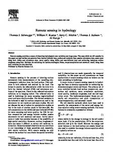
than 13 years providing an appropriate dataset for extended cohort studies for the areas with both high and level concentrations of ambient PM2.5. In addition, long-range transportation of particles as dust can provide potential vectors for bacteria (Ginoux and Torres, 2003; Prospero, 2003). With global coverage of this study, tracking PM2.5 transport is now easier for public health surveillance. Since many of the health conditions are interlinked, comprehensive studies are required to better understand the impact of PM2.5. With increasing availability of electronic health records, reliable PM2.5 data with seamless temporal and geographic coverage can contribute to revealing many unknowns of PM2.5 impacts on health. It could be noted that the type and degree of adverse effect greatly depends on the composition of the particulate matters. Composition mostly varies due to source materials. Our current study does not provide information on the composition of PM2.5. However, this study can be extended to examine the potential of source apportionment considering land use/land cover conditions and transportation mechanism. Recent studies show specific adverse impacts of exposure to ultrafine particles. Future studies are recommended to derive further size fractions beyond just PM2.5, particularly the ultra-fine particles in the sub-micron size range. The increasing awareness of the many health impacts implies the importance of having precise estimations of PM2.5. Existing remote sensing data can be effectively used to meet this need by employing ML, ensemble of random forests, to estimate the daily global PM2.5 abundance. The method utilizes remote sensing and meteorological data and ground-based observations of particulate matter at 3019 sites in 38 countries (see Fig. 2) (Lary et al., 2014a). Referring to Fig. 2, it can be observed that the sites in North America, Europe and Asia have higher density.

The health impacts of PM2.5 depend on its abundance at ground level where people can inhale the PM2.5. Various networks of ground-based sensors routinely measure the abundance of PM2.5. Fig. 2 indicates many gaps in the spatial coverage with no PM2.5 observations. This is mainly because of the poor coverage of the sensor network. This limitation has been tackled using remote sensing and satellite-derived Aerosol Optical Depth (AOD) coupled with numerical models (Engel-Cox et al., 2004a,b; Liu et al., 2007; Lee et al., 2011a,b). It has been proved that several parameters such as humidity, temperature, topography, cloud cover, and cloud optical depth affect the relationship between PM2.5 and AOD (e.g. Rajeev et al., 2008; Schaap et al., 2009; Liu and Harrison, 2011; Liu et al., 2012). Thus, a multivariate, non-linear and non-parametric ML approach seems to the best option to capture this relationship. ML has a very good performance in providing a new PM2.5 product. Fig. 3 presents the monthly average of the ML PM2.5 product (mg/m3). A good agreement exists between the PM2.5 product and the observations. In other words, the color fill of the circles depicting the observations is in good agreement with the background color depicting the new ML PM2.5 product. Careful attention to details is critical for the precision of PM2.5 simulations. First, a highly restrictive coincident requirement needs to be considered for the training dataset. Herein, we only take into account hourly PM2.5 and satellite observations that were made within 30 min of each other and had a great circle distance separation up to only 0.02" . Second, a comprehensive training dataset was gathered spanning the globe for more than a decade. Third, the use of the full range of training parameters that characterize the local environment as carefully as possible is recommended (e.g. humidity, temperature, boundary layer height, surface pressure, etc.). Fourth, a multivariate, nonlinear, nonparametric ML approach

Figure 2. The 8329 PM2.5 measurement site locations from 55 countries (red squares) that were used over the period 1997‒2014.

Please cite this article in press as: Lary, D.J., et al., Machine learning in geosciences and remote sensing, Geoscience Frontiers (2015), http:// dx.doi.org/10.1016/j.gsf.2015.07.003

D.J. Lary et al. / Geoscience Frontiers xxx (2015) 1e9

Figure 3. The monthly average ML PM2.5 product (mg/m#3) for August 2001 (Lary et al., 2014a).

is utilized that can handle continuous real variables and categorical variables (flags and masks). It is notable that remotely sensed AOD products typically have inherent biases relative to the ground truth from AERONET and are dependent on the remote sensing instrument, the algorithm, and the version of the processing software (collection). These biases were directly and individually calibrated for by performing separate ML training for our target variable (PM2.5) for each instrument, software version and algorithm combination (i.e. collection, deep blue, standard). Example of these separate calibrations can be seen in Fig. 4. 3.2. Dust sources Dust sources of many kinds are found globally. One of the most salient features of dust sources is that they are often very localized. For example, in Figs. 5 and 6, we can clearly see that the source of the dust plumes are best described as an ensemble of many point sources, not broad dust emitting regions. Realistically capturing this very localized nature of dust sources has so far largely eluded automated diagnosis, and consequently, description in global models. Invariably current models describe dust sources as rather large scale features (Ginoux et al., 2011), even when vegetation indices and similar approaches are used. This is in marked contrast to what we consistently see in the satellite imagery across the planet. Identifying dust sources is a critical yet challenging task for the accurate simulation of atmospheric particulate distributions (Ginoux et al., 2001; Prospero et al., 2002) relevant to air quality (Schauer et al., 1996) and climate change (Tegen and Lacis, 1996, Tegen et al., 1996). For this case, we take a new and radically different approach to any previous studies that have sought to identify global dust sources on a routine basis. We demonstrate that this new approach employing ML is very effective. The approach uses multi-

5

wavelength spectral reflectivity signatures to characterize land surfaces, naturally paving the way for a new class of algorithm ideally suited to fully exploit the next generation of hyper-spectral instrument. A common application of remote sensing is production of thematic maps using an image classification (Foody, 2002). New in our approach is that we can both operate at very high spatial resolution and distinguish between types of dust sources. For example, we can easily distinguish between the edge of salt flats (Fig. 6), dried up wadis or lakes, and agricultural sources to name just three of many examples. The only limiting factor for the resolution is the resolution of the satellite imagery. We employ ML to objectively provide an unsupervised multivariate and nonlinear classification into a very large number of surface types (in our demonstration study presented below 1000 classes are used) using multi-spectral satellite data. In other words, we do not impose any a priori assumptions, but rather, we let the data speak for itself as to how we should classify surface types. Self-organizing maps (SOMs) are good candidates to handle this classification task. SOMs are a data visualization and unsupervised classification technique invented by Kohonen (1982). They reduce the dimensions of data through the use of self-organizing neural networks. SOMs help us address the issue that humans simply cannot visualize high dimensional data unaided. The way SOMs go about reducing dimensionality is by producing a feature map, usually with two dimensions, that objectively plots the similarities of the data by grouping similar data items together. SOMs learn to classify input vectors according to how they are grouped in the input space. The SOM learns to recognize neighboring sections of the input space. Thus, SOMs learn both the distribution and topology of the input vectors they are trained on. This approach allows SOMs to display similarities and reduce the dimensionality. A SOM does not assume a priori a functional form for the analyzed data. A noteworthy enhancement of an SOM over principal component analysis is an SOM’s ability to represent non-linear functions or mappings. For further details please refer to Kohonen (1982). The premise being that there are very many types of dust sources, from the diatom rich sediments of the Bodélé depression in Chad, to those at the edge of salt flats in Bolivia and Chile (Fig. 5), to those in the coastal Green Mountains of Libya. Each of these dust sources has distinct physical characteristics, and therefore a distinct reflectance signature. If we are able to identify these signatures, then we can map the temporal and spatial evolution of each of these distinct dust sources. Once we have the surface type classification, we then seek to identify which small subset of surface classes correspond to various kinds of dust sources. Once we have identified the signature of a wide variety of dust sources, we can precisely pick out these locations globally and how their distribution changes with time. This is particularly useful as dust sources are very localized, and some dust sources have a significant seasonal time evolution. Having a methodology to identify the signature of these small-scale regions is invaluable. The ML approach to dust source identification was first conceived in 2010 to face a very practical challenge that the Navy has in producing real time visibility forecasts (Walker et al., 2009). If the standard type of dust sources are used (Ginoux et al., 2001), very poor regional visibility forecasts result. However, the quality of the Navy visibility forecasts drastically improved with an analyst (Annette Walker) manually identifying individual dust sources at the heads of plumes by examining sequences of satellite images such as those shown in Fig. 5 and also the EUMETSAT RGB Composites Dust images available online (http://oiswww.eumetsat.org/ IPPS/html/MSG/RGB/DUST/). This methodology is very labor intensive and does not lend itself to easy automation. The first prototype dust sources using the ML approach described here were devised specifically to automate the dust source identification and

Please cite this article in press as: Lary, D.J., et al., Machine learning in geosciences and remote sensing, Geoscience Frontiers (2015), http:// dx.doi.org/10.1016/j.gsf.2015.07.003

6

D.J. Lary et al. / Geoscience Frontiers xxx (2015) 1e9

Figure 4. The quality of the ML fits is always quantified by scatter diagrams of the observed “truth” plotted on the x-axis against the corresponding ML estimate plotted on the y-axis. A separate ML fits of PM2.5 is performed for each satellite data product using a given algorithm and instrument.

also allow for the accurate diagnosis of the time evolution in the spatial extent of the dust sources. Beyond the applications of accurate dust sources for visibility and air quality forecasts, the radiative forcing (RF) due to dust is a key concept in climate change calculations considered by the IPCC for the quantitative comparison of the strength of different human and natural agents causing climate change (Solomon et al., 2007). Radiative forcing can be categorized into direct and indirect effects. A significant part of the direct effect is the mechanism by which aerosols scatter and absorb shortwave and longwave radiation, thereby altering the radiative balance of the Eartheatmosphere system. Mineral dust is a major component of global aerosols that

Figure 5. Dust sources are typically localized point sources.

Figure 6. Examples of our ML approach correctly identifying very localized point sources around the edge of salt flats in Bolivia and Chile. Notice the narrow dust plumes originating from precisely the identified source regions that have been highlighted in blue and cyan.

Please cite this article in press as: Lary, D.J., et al., Machine learning in geosciences and remote sensing, Geoscience Frontiers (2015), http:// dx.doi.org/10.1016/j.gsf.2015.07.003

D.J. Lary et al. / Geoscience Frontiers xxx (2015) 1e9

exert a significant direct radiative forcing. Mineral dust aerosols are produced both naturally (z70%) and anthropogenically (z30%). As discussed above, the main goal is to determine all dust source surface locations on the planet. To this aim, SOM was used to classify all the land surface locations into a very large set of n categories. In the examples shown here, n ¼ 1000. A small subset of these 1000 categories will be regions that are dust sources. Naturally, there are a variety of distinct types of dust sources (e.g. dry river beds, agricultural sources, edge of salt flats, etc.) that we would like to delineate. To achieve a comprehensive classification, we want to consider the conditions present throughout the year, therefore, in the demonstration, we took an entire year of the 0.05" MCD43C3 data product. For this entire year of data, we then calculate the mean, m for each grid point. This is a massive dataset, and the computational time and memory required to perform the SOM classification increases with the number of data records. For the examples shown here, we therefore first restricted our attention to those broad MODIS surface types that may include dust sources, namely: barren or sparsely vegetated surfaces, croplands, grasslands, and open and closed shrublands. These are MODIS surface types 16, 12, 10, 7 and 6, respectively. For each of these surface types, we then constructed an input vector that contains 7 values, namely for each of the 7 bands provided in the MCD43C3 MODIS product the mean, m, of the directional and bihemispherical reflectance. When training the SOM algorithm, we used the Euclidean distance to compare the input vectors (each containing 7 values). In order to provide a fine gradation of classification, we used the SOM to group together the surface locations into 1000 classes, only a small subset of which correspond to regions that are dust sources. Once the classes that correspond to dust sources have been successfully identified, we have an automated method with which we can identify dust sources that can be routinely executed to provide a regular dust source data product. We utilized the extensive hand classification of very localized dust sources produced by the Navy (Walker et al., 2009) for the Middle East and South West Asia to guide our initial determination of which of the 1000 classes are dust sources. It is worth noting that the SOM classes are unique and distinct. 3.2.1. Bolivia and Chile salt flats dust event Let us examine a case study. Fig. 6 shows the dust event of July 18, 2010 in the Bolivian Altiplano. This event can be seen clearly in the MODIS Aqua True Color image where dust plumes emanate from fluvio-lacustine deposits and fluviodeltaic sediments (Risacher and Fritz, 1991a, b) around the Salars de Coipasa and Uyuni, Lake Poopo, and other smaller salt flats and lakes. Overlaid are the SOM classes that coincide with active dust sources on the Altiplano. Notice that the salt flats themselves are not dust sources, rather we see the plumes forming around the edges of the flats and lakes. SOMs are very successful in identifying the unique spectral signatures of dust sources. A set of papers is in preparation will be describing an exhaustive atlas of the global dust sources. 4. Conclusion and future direction We have discussed the main areas where ML can make a major impact in geosciences and remote sensing. ML focuses on the automatically extraction of information from data by computational and statistical methods. Herein, the features of the ML techniques for nonparametric regression and classification purposes are outlined. The ML’s application areas are very diverse and include different themes such as trace gases, aerosol products, vegetation indices, ocean products, characterization of rock mass, liquefaction phenomenon, ground motion parameters, interpreting

7

the remote sensing image, etc. We also presented a review of a number of recent applications of the new GP method in the field. Two illustrative examples are presented to demonstrate the efficiency of ML for tackling the geosciences and remote sensing problems. Currently, data analysis methods play a central role in geosciences and remote sensing. While gathering large collections of data is essential in the field, analyzing this information becomes more challenging. Evidently, such “Big Data” has notable effects both on the predictive analytics and the knowledge extraction and interpretation tools. Considering the significant capabilities of ML, it seems to be a very efficacious approach to handle this type of information.

References Alavi, A.H., Gandomi, A.H., 2012. Energy-based models for assessment of soil liquefaction. Geoscience Frontiers 3 (4), 541e555. Alavi, A.H., Gandomi, A.H., Modaresnezhad, M., Mousavi, M., 2011b. New groundmotion prediction equations using multi expression programming. Journal of Earthquake Engineering 15 (4), 511e536. Alavi, A.H., Gandomi, A.H., 2011. A robust data mining approach for formulation of geotechnical engineering systems. Engineering Computations 28 (3), 242e274. Alavi, A.H., Ameri, M., Gandomi, A.H., Mirzahosseini, M.R., 2011a. Formulation of flow number of asphalt mixes using a hybrid computational method. Construction and Building Materials 25 (3), 1338e1355. Alavi, A.H., Gandomi, A.H., Sahab, M.G., Gandomi, M., 2010. Multi expression programming: a new approach to formulation of soil classification. Engineering with Computers 26 (2), 111e118. Allen, M.R., Stott, P.A., Mitchell, J.F.B., Schnur, R., Delworth, T.L., 2000. Quantifying the uncertainty in forecasts of anthropogenic climate change. Nature 407 (6804), 617e620. Atkinson, P.M., Tatnall, A.R.L., 1997. Introduction: neural networks in remote sensing. International Journal of Remote Sensing 18 (4), 699e709. Ayala, A., Brauer, M., Mauderly, J.L., Samet, J.M., 2012. Air pollutants and sources associated with health effects. Air Quality Atmosphere and Health 5 (2), 151e167. http://dx.doi.org/10.1007/s11869-011-0155-2. Azamathulla, H.M., Ghani, A.A., Fei, S.Y., 2012. ANFIS-based approach for predicting sediment transport in clean sewer. Applied Soft Computing 12 (3), 1227e1230. Azamathulla, H.M., Guven, A., Demir, Y.K., 2011. Linear genetic programming to scour below submerged pipeline. Ocean Engineering 38 (8e9), 995e1000. Azamathulla, H.M., Wu, F.C., 2011. Support vector machine approach for longitudinal dispersion coefficients in natural streams. Applied Soft Computing 11 (2), 2902e2905. Azamathulla, H.M., 2012. Linear programming for irrigation scheduling e a case study (Book Chapter). In: Linear Programming: New Frontiers in Theory and Applications, pp. 174e192. Baykasoglu, A., Gullu, H., Canakci, H., Ozbakir, L., 2008. Prediction of compressive and tensile strength of limestone via genetic programming. Expert Systems with Applications 35 (1e2), 111e123. Beiki, M., Bashari, A., Majdi, A., 2010. Genetic programming approach for estimating the deformation modulus of rock mass using sensitivity analysis by neural network. International Journal of Rock Mechanics and Mining Sciences 47, 1091e1103. Boldo, E., Linares, C., Lumbreras, J., Borge, R., Narros, A., Garcia-Perez, J., FernandezNavarro, P., Perez-Gomez, B., Aragones, N., Ramis, R., Pollan, M., Moreno, T., Karanasiou, A., Lopez-Abente, G., 2011. Health impact assessment of a reduction in ambient PM2.5 levels in spain. Environment International 37 (2), 342e348. http://dx.doi.org/10.1016/j.envint.2010.10.004. Brook, R.D., Rajagopalan, S., Pope, I., Arden, C., Brook, J.R., Bhatnagar, A., DiezRoux, A.V., Holguin, F., Hong, Y., Luepker, R.V., Mittleman, M.A., Peters, A., Siscovick, D., Smith, J., Sidney, C., Whitsel, L., Kaufman, J.D., E. Amer Heart Assoc Council, D. Council Kidney Cardiovasc, M. Council Nutr Phys Activity, 2010. Particulate matter air pollution and cardiovascular disease an update to the scientific statement from the American heart association. Circulation 121 (21), 2331e2378. http://dx.doi.org/10.1161/CIR.0b013e3181dbece1. Brown, M.E., Lary, D.J., Vrieling, A., Stathakis, D., Mussa, H., 2008. Neural networks as a tool for constructing continuous NDVI time series from AVHRR and MODIS. International Journal of Remote Sensing 29 (24), 7141e7158. Cabalar, A.F., Cevik, A., 2009. Genetic programming-based attenuation relationship, an application of recent earthquakes in turkey. Computers & Geosciences 35 (9), 1884e1896. Carpenter, G.A., Gjaja, M.N., Gopal, S., Woodcock, C.E., 1997. Art neural networks for remote sensing: vegetation classification from landsat tm and terrain data. IEEE Transactions on Geoscience and Remote Sensing 35 (2), 308e325. Chen, L., Yeh, K., Wei, H., Liu, G., 2011. An improved genetic programming to SSM/I estimation typhoon precipitation over ocean. Hydrol Process 25, 2573e2583. Chen, L., 2003. A study of applying genetic programming to reservoir trophic state evaluation using remote sensor data. International Journal of Remote Sensing 24 (11), 2265e2275.

Please cite this article in press as: Lary, D.J., et al., Machine learning in geosciences and remote sensing, Geoscience Frontiers (2015), http:// dx.doi.org/10.1016/j.gsf.2015.07.003

8

D.J. Lary et al. / Geoscience Frontiers xxx (2015) 1e9

Chuang, M.-T., Zhang, Y., Kang, D., 2012. Application of wrf/chem-madrid for realtime air quality forecasting over the southeastern united states (vol 45, pg 6241, 2011). Atmospheric Environment 60, 677e678. Das, S.K., Basudhar, P.K., 2008. Prediction of residual friction angle of clays using artifical neural network. Engineering Geology 100 (3e4), 142e145. Dockery, D.W., Pope, C.A., Xu, X.P., Spengler, J.D., Ware, J.H., Fay, M.E., Ferris, B.G., Speizer, F.E., 1993. An association between air-pollution and mortality in 6 united-states cities. New England Journal of Medicine 329 (24), 1753e1759. http://dx.doi.org/10.1056/nejm199312093292401. //WOS: A1993MK09600001. dos Santos, J.A., Faria, F.A., Calumby, R.T., Torres, R., da, S., Lamparelli, R.A.C., July 2010. A genetic programming approach for coffee crop recognition. In: IGARSS 2010. Honolulu, USA, pp. 3418e3421. Engel-Cox, J.A., Hoff, R.M., Haymet, A.D.J., 2004a. Recommendations on the use of satellite remote-sensing data for urban air quality. Journal of the Air & Waste Management Association 54 (11). Engel-Cox, J.A., Holloman, C.H., Coutant, B.W., Hoff, R.M., 2004b. Qualitative and quantitative evaluation of MODIS satellite sensor data for regional and urban scale air quality. Atmospheric Environment 38 (16). Foody, G.M., 2002. Status of land cover classification accuracy assessment. Remote Sensing of Environment 80 (1), 185e201. http://dx.doi.org/10.1016/S00344257(01)00295-4. Gandomi, A.H., Alavi, A.H., Mousavi, M., Tabatabaei, S.M., 2011. A hybrid computational approach to derive new ground-motion prediction equations. Engineering Applications of Artificial Intelligence 24 (4), 717e732. Gandomi, A.H., Alavi, A.H., 2013. Hybridizing genetic programming with orthogonal least squares for modeling of soil liquefaction. International Journal of Earthquake Engineering and Hazard Mitigation 1 (1), 1e8. Gandomi, A.H., Alavi, A.H., 2011. Multi-stage genetic programming: a new strategy to nonlinear system modeling. Information Sciences 181 (23), 5227e5239. Garg, A., Garg, Ankit, Tai, K., Sreedeep, S., 2014a. An integrated SRM-multi-gene genetic programming approach for prediction of factor of safety of 3-D soil nailed slopes. Engineering Applications of Artificial Intelligence 30, 30e40. Garg, A., Tai, K., Savalani, M.M., 2014b. State-of-the-Art in empirical modeling of rapid prototyping processes. Rapid Prototyping Journal 20 (2), 164e178. Garg, A., Tai, K., Gupta, A.K., 2014c. A modified multi-gene genetic programming approach for modelling true stress of dynamic strain aging regime of austenitic stainless steel 304. Meccanica 49 (5), 1193e1209. Ginoux, P., Chin, M., Tegen, I., Prospero, J.M., Holben, B., Dubovik, O., Lin, S.J., 2001. Sources and distributions of dust aerosols simulated with the GOCART model. Journal of Geophysical Research-Atmospheres 106 (D17), 20255e20273. Ginoux, P., Torres, O., 2003. Empirical TOMS index for dust aerosol: applications to model validation and source characterization. Journal of Geophysical ResearchAtmospheres 108 (D17). http://dx.doi.org/10.1029/2003jd003470. Grell, G.A., Peckham, S.E., Schmitz, R., McKeen, S.A., Frost, G., Skamarock, W.C., Eder, B., 2005. Fully coupled “online” chemistry within the WRF model. Atmospheric Environment 39 (37), 6957e6975. Hansen, J., Fung, I., Lacis, A., Rind, D., Lebedeff, S., Ruedy, R., Russell, G., Stone, P., 1988. Global climate changes as forecast by Goddard institute for space studies 3-dimensional model. Journal of Geophysical Research-Atmospheres 93 (D8), 9341e9364. IPCC, 2013. Climate Change 2013: The Physical Science Basis. Contribution of Working Group I to the Fifth Assessment Report of the Intergovernmental Panel on Climate Change. Cambridge University Press, Cambridge. Javadi, A.A., Rezania, M., Nezhad, M.M., 2006. Evaluation of liquefaction induced lateral displacements using genetic programming. Computers and Geotechnics 33 (4e5), 222e233. Karakus, M., 2011. Function identification for the intrinsic strength and elastic properties of granitic rocks via genetic programming (GP). Computers & Geosciences 37, 1318e1323. Kohonen, T., 1982. Self-organized formation of topologically correct feature maps. Biological Cybernetics 43 (1), 59e69. Koza, J., 1992. Genetic Programming, on the Programming of Computers by Means of Natural Selection. MIT Press, Cambridge (MA). Lary, D.J., Remer, L.A., MacNeill, D., Roscoe, B., Paradise, S., 2009. Machine learning and bias correction of MODIS aerosol optical depth. IEEE Geoscience and Remote Sensing Letters 6 (4), 694e698. Lary, D.J., Muller, M.D., Mussa, H.Y., 2004. Using neural networks to describe tracer correlations. Atmospheric Chemistry and Physics 4, 143e146. Lary, D.J., Faruque, F., Malakar, N., Moore, A., Roscoe, B., Adams, Z., Eggelston, Y., 2014a. Estimating the global abundance of ground level presence of microscopic particulate matter. Geospatial Health 8, S611eS630. Lary, D.J., 2010. Artificial intelligence in geoscience and remote sensing. In: Imperatore, P., Riccio, D. (Eds.), Geoscience and Remote Sensing, New Achievements. IN-TECH, Vukovar, Croatia, pp. 1e24. Lary, D.J., Waugh, D.W., Douglass, A.R., Stolarski, R.S., Newman, P.A., Mussa, H., 2007. Variations in stratospheric inorganic chlorine between 1991 and 2006. Geophysical Research Letters 34. Lee, H.J., Liu, Y., Coull, B., Schwartz, J., Koutrakis, P., 2011a. PM2.5 prediction modeling using MODIS AOD and its implications for health effect studies. Epidemiology 22 (1). Lee, H.J., Liu, Y., Coull, B.A., Schwartz, J., Koutrakis, P., 2011b. A novel calibration approach of MODIS AOD data to predict PM2.5 concentrations. Atmospheric Chemistry and Physics 11 (15).

Lewkowski, C., Porwal, A., González-Álvarez, I., 2010. Genetic programming applied to base-metal prospectivity mapping in the Aravalli Province, India. Geophysical Research Abstracts 12, EGU2010e15171. Lia, W.X., Daib, L.F., Houa, X.B., Leia, W., 2007. Fuzzy genetic programming method for analysis of ground movements due to underground mining. International Journal of Rock Mechanics and Mining Sciences 44, 954e961. Liu, Y., Franklin, M., Kahn, R., Koutrakis, P., 2007. Using aerosol optical thickness to predict ground-level PM2.5 concentrations in the St. Louis area: a comparison between MISR and MODIS. Remote Sensing of Environment 107 (1e2). Liu, Y., He, K., Li, S., Wang, Z., Christiani, D.C., Koutrakis, P., 2012. A statistical model to evaluate the effectiveness of PM2.5 emissions control during the beijing 2008 olympic games. Environment International 44. Liu, Y.-J., Harrison, R.M., 2011. Properties of coarse particles in the atmosphere of the united kingdom. Atmospheric Environment 45 (19). Madadi, M.R., Azamathulla, H. Md, Yakhkeshi, M., 2015. Application of Google Earth to investigate the change of flood inundation area due to flood detention dam. Earth Science Informatics. http://dx.doi.org/10.1007/s12145-014-0197-8. Makkeasorn, A., Chang, N.B., Li, J., 2009. Seasonal change detection of riparian zones with remote sensing images and genetic programming in a semi-arid watershed. Journal of Environmental Management 90, 1069e1080. Makkeasorn, A., Chang, N.B., Beaman, M., Wyatt, C., Slater, C., 2006. Soil moisture estimation in a semi-arid watershed using RADARSAT-1 satellite imagery and genetic programming. Water Resources Research 42, 1e15. Nikravesh, M., 2007. Computational intelligence for geosciences and oil exploration. In: Forging New Frontiers: Fuzzy Pioneers I, vol. 66. California University Press, pp. 267e332. Ozbek, A., Unsal, M., Dikec, A., 2013. Estimating uniaxial compressive strength of rocks using GEP. Journal of Rock Mechanics and Geotechnical Engineering 5, 325e329. Pope, C., Dockery, A.,D.W., 2006. Health effects of fine particulate air pollution: lines that connect. Journal of the Air & Waste Management Association 56 (6), 709e742. Pope, I., Arden, C., Burnett, R.T., Krewski, D., Jerrett, M., Shi, Y., Calle, E.E., Thun, M.J., 2009. Cardiovascular mortality and exposure to airborne fine particulate matter and cigarette smoke shape of the exposure-response relationship. Circulation 120 (11), 941e948. http://dx.doi.org/10.1161/circulationaha.109.857888. Prospero, J.M., Ginoux, P., Torres, O., Nicholson, S.E., Gill, T.E., 2002. Environmental characterization of global sources of atmospheric soil dust identified with the nimbus 7 total ozone mapping spectrometer (TOMS) absorbing aerosol product. Reviews of Geophysics 40 (1), 31. Prospero, J.M., 2003. Global dust transport over the oceans: the link to climate. Geochimica Et Cosmochimica Acta 67 (18). A384eA384. Rajeev, K., Parameswaran, K., Nair, S.K., Meenu, S., 2008. Observational evidence for the radiative impact of Indonesian smoke in modulating the sea surface temperature of the equatorial Indian Ocean. Journal of Geophysical Research-Atmospheres 113 (D17). Ravandi, E.G., Rahmannejad, R., Feili Monfared, A.E., Ravandid, E.G., September 2013. Application of numerical modeling and genetic programming to estimate rock mass modulus of deformation. International Journal of Mining Science and Technology 23 (5), 733e737. Risacher, F., Fritz, B., 1991a. Geochemistry of bolivian salars, lipez, southern altiplano origin of solutes and brine evolution. Geochimica Et Cosmochimica Acta 55 (3), 687e705. Risacher, F., Fritz, B., 1991b. Quaternary geochemical evolution of the salars of uyuni and coipasa, central altiplano, bolivia. Chemical Geology 90 (3e4), 211e231. Rosin, P., Hervas, J., 2002. Image thresholding for landslide detection by genetic programming. In: Bruzzone, L., Smiths, P. (Eds.), Analysis of Multi-temporal Remote Sensing Images. World Scientific, pp. 65e72. Samui, P., 2008a. Support vector machine applied to settlement of shallow foundations on cohesionless soils. Computers and Geotechnics 35 (3), 419e427. Samui, P., 2008b. Slope stability analysis: a support vector machine approach. Environmental Geology 56 (2), 255e267, 35. Samui, P., 2012. Application of statistical learning algorithms to ultimate bearing capacity of shallow foundation on cohesionless soil. International Journal for Numerical and Analytical Methods in Geomechanics 36 (1), 100e110. Schaap, M., Apituley, A., Timmermans, R.M.A., Koelemeijer, R.B.A., de Leeuw, G., 2009. Exploring the relation between aerosol optical depth and PM2.5 at Cabauw, the Netherlands. Atmospheric Chemistry and Physics 9 (3). Schauer, J., Rogge, W., Hildemann, L., Mazurek, M., Cass, G., Simoneit, B., 1996. Source apportionment of airborne particulate matter using organic compounds as tracers. Atmospheric Environment 30 (22), 3837e3855. Shahin, M.A., Jaksa, M.B., 2005. Neural network prediction of pullout capacity of marquee ground anchors. Computers and Geotechnics 32 (3), 153e163. Shahin, M.A., Jaksa, M.B., Maier, H.R., 2001. Artificial neural network applications in geotechnical engineering. Australian Geomechanics 36 (1), 49e62. Shuhua, Z., Qian, G., Jianguo, S., 2006. Genetic programming approach for predicting surface subsidence induced by mining. Journal of China University of Geosciences 17 (4), 361e366. Solomon, S., Qin, D., Manning, M., Chen, Z., Marquis, M., Averyt, K., Tignor, M., Miller, H., 2007. IPCC Fourth Assessment Report: Climate Change 2007. Cambridge University Press, Cambridge. Tegen, I., Lacis, A., Fung, I., 1996. The influence of mineral aerosols from disturbed soils on the global radiation budget. Nature 380, 419e422.

Please cite this article in press as: Lary, D.J., et al., Machine learning in geosciences and remote sensing, Geoscience Frontiers (2015), http:// dx.doi.org/10.1016/j.gsf.2015.07.003

D.J. Lary et al. / Geoscience Frontiers xxx (2015) 1e9 Tegen, I., Lacis, A., 1996. Modeling of particle size distribution and its influence on the radiative properties of mineral dust aerosol. Journal of Geophysical Research 101, 19237e19244. Walker, A.L., Liu, M., Miller, S.D., Richardson, K.A., Westphal, D.L., 2009. Development of a dust source database for mesoscale forecasting in southwest Asia. Journal of Geophysical Research-Atmospheres 114. WHO, 2014. 7 million Premature Deaths Annually Linked to Air Pollution. URL: http://www.who.int/mediacentre/news/releases/2014/air-pollution/en/.

9

Yi, J.S., Prybutok, V.R., 1996. A neural network model forecasting for prediction of daily maximum ozone concentration in an industrialized urban area. Environmental Pollution 92 (3), 349e357. Zahabiyoun, B., Goodarzi, M.R., Bavani, A.R.M., Azamathulla, H.M., 2013. Assessment of climate change impact on the Gharesou river Basin using SWAT Hydrological model. Clean e Soil, Air, Water 41 (6), 601e609.

Please cite this article in press as: Lary, D.J., et al., Machine learning in geosciences and remote sensing, Geoscience Frontiers (2015), http:// dx.doi.org/10.1016/j.gsf.2015.07.003