Mathematical Formula Recognition using Machine Learning Techniques

Mathematical Formula Recognition using Machine Learning Techniques

Théodore Bluche under the Supervision of Dr. Vasile Palade

Dissertation submitted for the completion of the

MSc in Computer Science Worcester College

University of Oxford

September 3, 2010

2

Abstract

Unlike texts, printed mathematical expressions have a two-dimensional nature, and their recognition involves the recognition of the structure of the formula and of the symbols contained in it. In most research, the structure recognition uses the identity of symbols. Moreover, a few previous works use the structure in the symbol recognition, or machine learning techniques in the structure recognition part. There is a lot of mathematical symbols, they can be very similar, and new symbols are being invented by scientists. The arrangements of symbols, however, evolve less. In this dissertation, we investigate the possibility of recognizing the structure of the mathematical expression without the symbols’ identity. We also perform a prior classification of the symbols using the structure only. Moreover, we use very few knowledge about mathematical expression syntax. This approach has, to the best of our knowledge, never been tried. We built a system using machine learning techniques, such as neural networks and fuzzy logic. A binary image representing a mathematical expression is segmented, and the recognition is performed using the symbols’ bounding boxes. An iterative algorithm using a multi-classifier system recognizes the structure and classifies the symbols. The results proved that the context of a symbol, when known and used, can help classify the symbol. The structure recognition using a non-recursive algorithm with very few backtracking yielded good results. This project proved that the symbols’ identity is not essential for the structure analysis. Moreover, the structure recognition provides some useful information for the symbol classification. This classification is assumed to help the symbol recognition in a future work. Finally, the machine learning approach produced a flexible system, able to adapt to unknown symbols and writing styles, and to return confidence values for the recognition, rather than a crisp interpretation.

3

4

Acknowledgements

I owe my deepest gratitude to my supervisor, Vasile Palade, for the guidance and support he gave me thoughout this project. His advice and experience have greatly helped me focus on the important points and write this dissertation. It is an honor to thank Dr. Dorothea Blostein, who published several papers on the subject, and who pointed me out the Infty data set. I owe a special acknowledgement to Dr. Claudie Faure, researcher in ENST ParisTech. She made available to me two papers she published, which I could not find. I am very grateful for she showed great interest in my project, and replied all my emails quickly. I would also like to thank Laurence Likforman, who interviewed me during a PhD application, and then sent me an interesting paper related to my project [18]. This thesis could not have been complete without the help of the persons who have completed the online quiz for manual equations labelling. I collected more answers than expected, and some people even sent me suggestions about the presentation of the quiz. I would like to show my gratitude to my academic supervisor, Bernard Sufrin. I enjoyed our conversations, and his support has been of immeasurable value. His encouragement and guidance thoughout the masters allowed me to take pleasure in studying in Oxford. I also want to take this opportunity to thank the teachers, staff and students of the Computing Laboratory, and of Worcester College, for their assistance and friendship, and without whom the experience of being a student in Oxford would not have been complete. I owe an acknowledgement to Supélec, the engineering school in which I studied last year. They helped me applying to Oxford University. I would like to address a special thanks to Anne Chrétien, for her recommendations and support, and my referees Yolaine Bourda, Alain Destrez and Fran¸coise Brouaye. I would like to thank my uncle Olivier, who shared with me his experience living in England and helped me applying to Oxford University Finally, I am indebted to my family for they made this fulfiling experience possible by funding my MSc. They have been of great support when I encountered difficulties, from the application process to the end of the project.

5

6

Contents Abstract

2

Acknowledgements

3

1 Introduction 1.1 Description of the Problem . . . . . . . . . . . . . . . . . . . . . . . . . . . 1.2 Project Aims . . . . . . . . . . . . . . . . . . . . . . . . . . . . . . . . . . . 1.3 Structure of the Thesis . . . . . . . . . . . . . . . . . . . . . . . . . . . . . .

11 11 12 13

2 Background 2.1 Mathematical Notations . . . . . . . . . . . . . . . . . 2.1.1 Writing and Reading a Mathematical Formula 2.1.2 Problems posed by Mathematical Expressions . 2.1.3 Representing a Formula . . . . . . . . . . . . . 2.2 Mathematical Formula Recognition . . . . . . . . . . . 2.2.1 Symbol Recognition . . . . . . . . . . . . . . . 2.2.2 Structure Recognition . . . . . . . . . . . . . . 2.3 Review of Existing Techniques . . . . . . . . . . . . .

. . . . . . . .

. . . . . . . .

. . . . . . . .

. . . . . . . .

. . . . . . . .

. . . . . . . .

. . . . . . . .

. . . . . . . .

3 Motivations and Method Overview 3.1 Motivations and Hypothesis for a New Approach . . . . . . . . . . . 3.1.1 Motivations . . . . . . . . . . . . . . . . . . . . . . . . . . . . 3.1.1.1 Apparent simplicity of the structure recognition . . 3.1.1.2 Mathematical symbols are sometimes complicated . 3.1.2 Hypothesis . . . . . . . . . . . . . . . . . . . . . . . . . . . . 3.2 Scope of the project . . . . . . . . . . . . . . . . . . . . . . . . . . . 3.2.1 Complexity of Mathematical Expressions . . . . . . . . . . . 3.2.2 Extent of the Project . . . . . . . . . . . . . . . . . . . . . . 3.2.3 Limitations . . . . . . . . . . . . . . . . . . . . . . . . . . . . 3.3 Method Overview . . . . . . . . . . . . . . . . . . . . . . . . . . . . . 3.3.1 Presentation of the Proposed System . . . . . . . . . . . . . . 3.3.2 Pre-processing . . . . . . . . . . . . . . . . . . . . . . . . . . 3.3.3 Symbol Classification . . . . . . . . . . . . . . . . . . . . . . 3.3.3.1 Rough Classification . . . . . . . . . . . . . . . . . . 3.3.3.2 Classification using Context . . . . . . . . . . . . . 3.3.4 Structure Recognition . . . . . . . . . . . . . . . . . . . . . . 3.3.4.1 A Neural-Network based Relationship Classifier . . 3.3.4.2 Finding Children in Class-Dependant Fuzzy Regions 3.3.4.3 Extracting Lines using Fuzzy Baselines . . . . . . . 3.3.4.4 Recognizing the Structure . . . . . . . . . . . . . . . 3.3.5 An Iterative Process for the Whole Recognition . . . . . . . . 7

. . . . . . . .

. . . . . . . .

. . . . . . . .

15 15 15 16 17 17 18 19 19

. . . . . . . . . . . . . . . . . . . . . . . .

. . . . . . . . . . . . . . . . . . . . .

. . . . . . . . . . . . . . . . . . . . .

25 25 25 25 25 26 28 28 29 29 31 31 32 33 33 34 35 35 36 37 37 38

. . . . . . . . . . . . . . . . . . . . . . . . .

8

CONTENTS

4 Design 4.1 Preliminary Work . . . . . . . . . . . . . . . . . . . . . . . . . . . . 4.1.1 Tools Used . . . . . . . . . . . . . . . . . . . . . . . . . . . 4.1.1.1 Tools for Analysis . . . . . . . . . . . . . . . . . . 4.1.1.2 Tools for Construction . . . . . . . . . . . . . . . . 4.1.1.3 Tools for Implementation . . . . . . . . . . . . . . 4.1.2 The Data Sets . . . . . . . . . . . . . . . . . . . . . . . . . 4.1.2.1 Overview of an Existing Data Set: Inf tyCDB − 1 4.1.2.2 Towards a New Data Set . . . . . . . . . . . . . . 4.1.3 Data analysis . . . . . . . . . . . . . . . . . . . . . . . . . . 4.1.3.1 Analysis of the Data on Relationships . . . . . . . 4.1.3.2 Analysis of the Data on Symbol Classes . . . . . . 4.2 Design of the System . . . . . . . . . . . . . . . . . . . . . . . . . . 4.2.1 Representation of the Data . . . . . . . . . . . . . . . . . . 4.2.2 Practical Design of the Classifiers . . . . . . . . . . . . . . . 4.2.2.1 Symbol Classifier . . . . . . . . . . . . . . . . . . . 4.2.2.2 Relationship Classifier . . . . . . . . . . . . . . . . 4.2.3 Functionalities of the System . . . . . . . . . . . . . . . . . 4.2.4 Integration of the Classifiers in an User-Friendly Interface . 4.2.4.1 Functionalities of the Interface . . . . . . . . . . . 4.2.4.2 Features of the Interface . . . . . . . . . . . . . . 4.3 Presentation of the Algorithms . . . . . . . . . . . . . . . . . . . . 4.3.1 Image Segmentation . . . . . . . . . . . . . . . . . . . . . . 4.3.2 The Recognition . . . . . . . . . . . . . . . . . . . . . . . . 4.3.2.1 Rough Symbol Classification . . . . . . . . . . . . 4.3.2.2 Structure Recognition . . . . . . . . . . . . . . . . 4.3.2.3 Symbol Classification using Context . . . . . . . . 4.3.2.4 The Iterations . . . . . . . . . . . . . . . . . . . . 4.3.3 Exporting the Results . . . . . . . . . . . . . . . . . . . . .

. . . . . . . . . . . . . . . . . . . . . . . . . . . .

. . . . . . . . . . . . . . . . . . . . . . . . . . . .

. . . . . . . . . . . . . . . . . . . . . . . . . . . .

. . . . . . . . . . . . . . . . . . . . . . . . . . . .

. . . . . . . . . . . . . . . . . . . . . . . . . . . .

39 39 39 40 40 40 41 41 42 46 46 47 49 49 53 54 58 64 67 67 68 70 70 70 71 71 72 73 74

5 Implementation 5.1 Implementation of the Expressions and Classifiers . . . . . 5.1.1 Implementation of the Expressions . . . . . . . . . 5.1.2 Implementation of the Classifiers . . . . . . . . . . 5.1.2.1 Trained classifiers . . . . . . . . . . . . . 5.1.2.2 Fuzzy Regions . . . . . . . . . . . . . . . 5.1.2.3 Fuzzy Baselines . . . . . . . . . . . . . . 5.1.2.4 Structure Recognizer . . . . . . . . . . . 5.1.3 Tools for the Analysis of the Classification Results 5.2 Additional Functionalities . . . . . . . . . . . . . . . . . . 5.3 Implementation of the Graphical User Interface (GUI) . . 5.3.1 Main Window . . . . . . . . . . . . . . . . . . . . . 5.3.2 Result View . . . . . . . . . . . . . . . . . . . . . . 5.3.2.1 ResultView . . . . . . . . . . . . . . . . . 5.3.2.2 RCWindow . . . . . . . . . . . . . . . . . 5.3.2.3 PlotWindow . . . . . . . . . . . . . . . . 5.3.3 Input Windows . . . . . . . . . . . . . . . . . . . . 5.3.4 File Manager . . . . . . . . . . . . . . . . . . . . . 5.4 Implementation of the Structure Recognition Algorithm . 5.4.1 BaselineStructure object . . . . . . . . . . . . . . . 5.4.2 The Stack of Last Symbols Seen . . . . . . . . . .

. . . . . . . . . . . . . . . . . . . .

. . . . . . . . . . . . . . . . . . . .

. . . . . . . . . . . . . . . . . . . .

. . . . . . . . . . . . . . . . . . . .

. . . . . . . . . . . . . . . . . . . .

77 77 77 79 79 81 81 81 82 82 82 83 84 84 84 85 86 87 88 88 89

6 Results and Evaluation

. . . . . . . . . . . . . . . . . . . .

. . . . . . . . . . . . . . . . . . . .

. . . . . . . . . . . . . . . . . . . .

. . . . . . . . . . . . . . . . . . . .

. . . . . . . . . . . . . . . . . . . .

91

CONTENTS

6.1

6.2 6.3

9

Parameters used for Evaluation . . . . . . . . . . . . . . 6.1.1 Recognition Errors . . . . . . . . . . . . . . . . . 6.1.2 Correctness Scores . . . . . . . . . . . . . . . . . 6.1.2.1 Symbol Correctness . . . . . . . . . . . 6.1.2.2 Relationship Correctness . . . . . . . . 6.1.3 Aggregating the Scores . . . . . . . . . . . . . . . Design of the Tests . . . . . . . . . . . . . . . . . . . . . 6.2.1 The Test Sets . . . . . . . . . . . . . . . . . . . . 6.2.2 Comparison with Human Labelling . . . . . . . . Performance of the System . . . . . . . . . . . . . . . . 6.3.1 Presentation of the Results . . . . . . . . . . . . 6.3.1.1 Overall . . . . . . . . . . . . . . . . . . 6.3.1.2 Per Test Set . . . . . . . . . . . . . . . 6.3.1.3 Human labelling . . . . . . . . . . . . . 6.3.2 Evaluation . . . . . . . . . . . . . . . . . . . . . 6.3.2.1 Scope of the Project and Flexibility . . 6.3.2.2 Evaluation of the Structure Recognition 6.3.2.3 Analysis of the Symbol Classification .

7 Conclusions 7.1 Findings . . . . . . . . . . . . . . . . . . 7.2 Evaluation . . . . . . . . . . . . . . . . . 7.3 Ideas for Further Development . . . . . 7.3.1 Improving the Training Set . . . 7.3.2 Improving the Recognition . . . 7.3.3 Extending the Proposed System

. . . . . .

. . . . . .

. . . . . .

. . . . . .

. . . . . .

. . . . . .

. . . . . .

. . . . . .

. . . . . .

. . . . . . . . . . . . . . . . . . . . . . . .

. . . . . . . . . . . . . . . . . . . . . . . .

. . . . . . . . . . . . . . . . . . . . . . . .

. . . . . . . . . . . . . . . . . . . . . . . .

. . . . . . . . . . . . . . . . . . . . . . . .

. . . . . . . . . . . . . . . . . . . . . . . .

. . . . . . . . . . . . . . . . . . . . . . . .

. . . . . . . . . . . . . . . . . . . . . . . .

. . . . . . . . . . . . . . . . . . . . . . . .

. . . . . . . . . . . . . . . . . .

. . . . . . . . . . . . . . . . . .

. . . . . .

107 . 107 . 108 . 108 . 109 . 109 . 110

Bibliography

91 91 92 92 93 94 95 95 96 100 100 100 101 103 103 103 104 104

110

A Implementation A.1 Main Functionalities of the System - Use Case View A.2 Package Organization . . . . . . . . . . . . . . . . . A.3 Methods in the Expression Implementation . . . . . A.4 Handling XML Files . . . . . . . . . . . . . . . . . . A.5 The Graphical User Interface (GUI) . . . . . . . . . A.5.1 The Menus . . . . . . . . . . . . . . . . . . . A.5.2 The Panels of the Main Window . . . . . . . A.5.3 Implementation of the ’Plot’ Window . . . . A.5.4 The File Manager . . . . . . . . . . . . . . . A.6 Implementation of Two Algorithms . . . . . . . . . . A.6.1 Data Set Creation . . . . . . . . . . . . . . . A.6.2 The Classification . . . . . . . . . . . . . . . A.6.2.1 Symbol Classification . . . . . . . . A.6.2.2 Structure Recognition . . . . . . . .

. . . . . . . . . . . . . .

. . . . . . . . . . . . . .

. . . . . . . . . . . . . .

. . . . . . . . . . . . . .

. . . . . . . . . . . . . .

. . . . . . . . . . . . . .

. . . . . . . . . . . . . .

. . . . . . . . . . . . . .

. . . . . . . . . . . . . .

. . . . . . . . . . . . . .

. . . . . . . . . . . . . .

. . . . . . . . . . . . . .

. . . . . . . . . . . . . .

115 115 115 117 118 118 118 120 120 121 121 121 122 122 122

B Algorithms B.1 Creation of the Data Sets B.2 Train the Classifiers . . . B.3 Segmentation . . . . . . . B.4 Parse Latex File . . . . . B.5 Symbol Classification . . . B.6 Structure Recognition . . B.7 Iterative Algorithm . . . .

. . . . . . .

. . . . . . .

. . . . . . .

. . . . . . .

. . . . . . .

. . . . . . .

. . . . . . .

. . . . . . .

. . . . . . .

. . . . . . .

. . . . . . .

. . . . . . .

. . . . . . .

125 125 126 127 129 129 130 133

. . . . . . .

. . . . . . .

. . . . . . .

. . . . . . .

. . . . . . .

. . . . . . .

. . . . . . .

. . . . . . .

. . . . . . .

. . . . . . .

. . . . . . .

. . . . . . .

. . . . . . .

. . . . . . .

. . . . . . .

10

CONTENTS

B.8 Export XML Interpretation . . . . . . . . . . . . . . . . . . . . . . . . . . . 133 B.9 Compare Expressions . . . . . . . . . . . . . . . . . . . . . . . . . . . . . . . 134 C Test Sets and Results 137 C.1 The Test Sets . . . . . . . . . . . . . . . . . . . . . . . . . . . . . . . . . . . 137 C.2 Notations and Figures . . . . . . . . . . . . . . . . . . . . . . . . . . . . . . 137 C.3 Results . . . . . . . . . . . . . . . . . . . . . . . . . . . . . . . . . . . . . . . 138

Chapter 1

Introduction First, we will briefly describe the problem of mathematical formula recognition. Then, we will state the aims of the project, and, finally, we will introduce the different parts of this document.

1.1

Description of the Problem

Today, as documents tend to be dematerialized to be stored on computer, systems able to transform a physical item into a digital one are needed. Most documents mainly contain text, either printed or handwritten. To this concern, Optical Character Recognition (OCR) has had tremendous improvements since the 1950s, leading to efficient pieces of software available nowadays. In particular, current technology allows one to enter a text by directly writing it on a data tablet, or touchscreen. While some may argue that typing a text is quicker than writing it, there is no doubt that it would be easier to write or scan a mathematical expression rather than inputting it using the available tools. For example, writing a complicated equation using Latex requires expertise, while the equation editors such as the one available in MS Word involve the selection of a symbol or a structure in a list, which constitutes a long process. Moreover, several printed documents, such as scientific papers or books, cannot be efficiently stored on a computer unless a system is able to recognize the mathematical formulae they contain. Plain texts and mathematical expressions are very different items. Text is a onedimensional sequence of characters, whereas mathematical expressions are a two-dimensional arrangement of symbols. Text contains letters and digits, whereas the number of symbols in equations is infinite. Moreover, in texts, single characters do not have a meaning of their own (except for acronyms). The smallest meaningful entity is the word, which is a sequence of characters. In mathematical expressions, each symbol has its meaning. In fact, mathematical expressions provide P a iconvenient way to communicate scientific concepts in a short and clear way. Indeed, i a looks somewhat simpler than ”the sum of all powers of the number a”. This example illustrate P also P j the fuzziness surrounding symbols. If a and i b refer to the same concept, i a and j b have exactly the same meaning. The set of expressions with that meaning is infinite, whereas in texts, characters are chosen to form words which are part of a vocabulary. Synonyms may exist but (i) in a finite number and (ii) they do not express the exact same idea. 11

12

CHAPTER 1. INTRODUCTION

The symbolic style of mathematical expressions drives scientific writers to explain what concept the symbols refer to. Indeed, the same symbol can have different meanings. For example, the capital Greek letter sigma (Σ) often refers to the summation, but might represent a set of object in a different context. Letters are sometimes variables which need to be described to be understood. These differences between text and mathematical expressions imply that their recognitions are dissimilar. In texts, characters can be recognized in a sequence and grouped to form words. A vocabulary can for instance help disambiguate the recognition. For mathematical expressions, the symbols must be recognized and the structure as well. Disambiguation is more complex because there is no such thing as a mathematical vocabulary. Although texts and mathematical expressions differ in their form, similar purposes exist for their recognition. This often corresponds to what extend one wants to understand the input. This includes: • the mere recognition of characters/symbols and their position to be able to reproduce the input on a computer, • the recognition of whole words and formulae to ensure a meaningful representation of the input, • the understanding of the input, for example using natural language processing for texts. For mathematical expressions, it corresponds to the understanding of the meaning of the symbols. The first published works on mathematical expression recognition date from the 1960s, but this field enjoyed significant research interest in the last two decades. The symbol recognition is either performed by classical OCR techniques, for instance using support vector machines [22], pattern matching [16, 24], or taken as granted (e.g. [28, 20, 2, 1, 9]). The structure analysis is mainly done using geometrical considerations, based on implicit rules (e.g. in [21, 28, 20, 27]) or grammar rules [17, 15, 8]. These rules take into account the identity of the symbol, and very few papers, such as [25], attempted to dissociate the structure analysis from the symbol recognition. The ambiguity in mathematical expressions, especially when handwritten, is commonly accepted. It can be an ambiguity on the symbol identity (e.g. q and 9 can look similar) or on the structure. Only some researches dealt with that problem, by keeping several interpretations on the symbol’s identity until the structure disambiguate it [17], or by producing several final interpretations, for the user to choose the best one [29]. Even though artifical intelligence can be found in the structure recognition, through fuzzy logic [29, 12], or search algorithms [9, 17, 18] (among others), machine learning is, to the best of our knowledge, rarely used in the structure analysis [1, 9].

1.2

Project Aims

The structure analysis of mathematical expressions varies from the mere recognition of spatial relationships (on the same line, exponent, and so on) to the real understanding of a formula. For example, Zanibbi et al. [28] perform a lexical and semantic analysis of the formula, enabling their system to recognize the function sinus rather than a triplet of symbols (’s’, ’i’, ’n’) on the same line. The semantic analysis is often used to recognize the

1.3. STRUCTURE OF THE THESIS

13

structure. For instance, some papers, such as [27], utilize the dominance and precedence of symbols to find the most likely relationships. Most papers use the identity of symbols to recognize the structure. For example, it allows to deduce the dominance of the symbol, and the regions where arguments, such as exponent, should be found. It also means that an error on the symbol recognition can have severe consequences on the structure analysis. In particular, mathematical notation evolve with the needs of scientists, and new symbols appear. These symbols might not be identified and compromise the structural analysis. This project investigates the possibility of performing the structural analysis and a symbol classification at the same time, using only very few knowledge about mathematical expression syntax. Our approach is based on the mutual constraint existing between symbols and structure. Indeed, knowing the symbols’ identity helps analyse the structure, but the structure can help disambiguate the symbol recognition ([17]). We aim to develop a system based on machine learning techniques, where the symbol classification and the structure analysis are separate tasks which constrain each other. Instead of identifying the symbols, we classify them according to a classification described in the literature (e.g. [28, 17]). Our contribution to the field consists in assuming that this classification can be performed using the symbols’ bounding boxes, and the structure of the expression only. We develop an iterative algorithm to exploit the constraints between both tasks. Our motivation is to define a method for building a system as flexible as possible and able to deal with the evolution of mathematical notation, and with the variation in the writing style. To do so, we implement machine learning artifacts, which allow us to return a soft interpretation, with confidence values, rather than a crisp one. The goal is to dissociate the structure recognition, which is the core of a mathematical expression recognizer, from the actual symbol identification, while providing results to improve the latter. Indeed, the classification of symbols constrains their identification, making it easier. Last but not least, we aim to achieve a very fast recognition of the structure. This implies a limited usage of backtracking, avoiding too much recursion, and a few comparisons between symbols only. This is a big challenge, given the nested two-dimensional nature of mathematical expressions.

1.3

Structure of the Thesis

This thesis is divided into seven chapters. • Chapter 1 introduces the project and its relation to the field of mathematical expression recognition. • Chapter 2 presents a background study about mathematical expressions in general, and their recognition by a computer program in particular. This is followed by a review of the literature in the area. • Chapter 3 explains our motivations and hypothesis for this new approach to mathematical formula recognition, and gives an overview of the method we proposed.

14

CHAPTER 1. INTRODUCTION

• Chapter 4 provides more details about the design of the system, that is the artifacts and parameters used, and presents the algorithms. • Chapter 5 focuses on the actual implementation of the system using object-oriented programming • Chapter 6 evaluates the results yielded by the implemented system and draws conclusions about the performance. • Chapter 7 concludes the dissertation, analysing how this approach can contribute to the field of recognition of mathematical expression, and giving ideas for further development. • Finally, the appendices provide more details about the developed system and its performance.

Chapter 2

Background In order to build a system able to recognize mathematical expressions, some preliminary work is necessary. We need to specify what is a mathematical expression. That means that we have to define how mathematical expressions are written, and how we read them. We have to investigate the different existing arrangements of symbols, and the corresponding meanings. Moreover, mathematical expressions can be used in different ways. They may be written for humans to easily read them. They are then put down as two-dimensional graphics. They may be written for computers to use it. The representation can vary, from the reverse polish notation used in 1980s handheld calculators, to tree structures in some symbolic computation systems today. For mathematical expression recognition, the notation which we want to understand is graphical. It poses some problem, such as understanding the relations between symbols. Indeed, they have a structure, used for mathematical communication between humans, independently from computers. This leads to the identification of the tasks involved in expression recognition, each having specific problems. Section 2.1 focuses on the mathematical notation and representation of the formulae in general. Section 2.2 explains what is mathematical expression recognition. Some research has been carried out in the past, especially in the last few years. Section 2.3 aims to review the state of the art in the field of mathematical formula recognition.

2.1

Mathematical Notations

A mathematical expression is not merely symbols put down in a random two-dimensional layout. It has a well-organized structure, which obeys the rules of the mathematical notation. The arrangement of two symbols with respect to each other conveys a certain meaning.

2.1.1

Writing and Reading a Mathematical Formula

The usual writing and reading order for mathematical expressions is left to right. Therefore, understanding a mathematical expression is not completely two-dimensional. Moreover, symbols in a relation are usually close to each other. For example, a subscript is very likely to be the closest symbol on the bottom right of its parent. In a few cases, the interpretation of a formula is possible only by reading the whole formula. For instance, we can fully understand an integration when we see the final dx. 15

16

CHAPTER 2. BACKGROUND

However, reading a mathematical expression is not straightforward, forP different symbols are usually read differently. This can be illustrated with some examples. ni=0 ai is usually read ”sum over i from 0 to n of a to the ith”. The pattern is operator, argument below, a argument above, argument on the same line. is read ”a over b”. The pattern in this b case is argument above, operator, argument under.

2.1.2

Problems posed by Mathematical Expressions

The major differences between plain text and mathematical expressions are: (i) there are far more symbols used in mathematical formulae, and (ii) there are more kinds of relationships in mathematical expressions. Those two points induce two main challenges in the recognition of mathematical expressions. The Number of Symbols Plain texts contain letters, digits and punctuation. There are some general rules such as ”capital letters are found at the beginning of a word” or ”digits are usually not mixed with letters in the same word”. Mathematical expressions can contain a wider range of symbols. Roman letters and digits are only a small subset. The Greek alphabet is often used, and a lot of mathematical symbols exist. It is impossible to list them, since scientists keep inventing new ones. Moreover, there are symbols which are similar in shape and appear in different contexts: Q • is the product symbol, whereas π is the Greek letter pi, • P is the capital letter while p is the small letter, • < is the operator ’lower than’ in 1 < 2 and a bracket in ha, bi • s is a variable in s3 whereas it is part of a function name in sin(

3π ) 2

or have distinct functions or meanings : • digits almost always represent numbers • letters can either be included in a function name, like n in sin(π), represent an precise object which is explained in a short text, as in ”O(n), , where n is the number of nodes”, P5 ornbe artifact to represent a more general concept, as the hidden variable n in n=0 x . • finally, most symbols are redefined for the need of the writer. The Spatial Relationships We can list six main spatial relationships: superscript (or top-right), subscript (or bottom-right), on the same line, above, under, inside. Once again, scientists may use new spatial arrangements when they need to, or give different meanings to existing relationships. For example, with the ’superscript’ relation, i is the power in xi , whereas (i) is an index in x(i) . The relation ’on the same line’ is even more complicated, for example: P • in a, a is an argument, • in 42, 4 and 2 are part of the same number,

2.2. MATHEMATICAL FORMULA RECOGNITION

17

• in an, the meaning is likely to be a × n • tan represents probably the ’tangent’ function • (i + 1) can be the argument of a function, of a product, and so on. While the meaning can differ from one case to another, the spatial behaviours associated with these relationships is fixed, and the translation in a Latex form is often the same for all these possibilities. Mathematical can generally be considered as nested structures, especially due to the a+1 existence and nature of spatial relationships. In , a + 1 and a − 1 are mathematical a−1 expressions on their own, nested in a more general one. As is 2xk in n2xk . Because formulae are globally written on a line, called baseline, the nested structure implies the existence nested baselines. The nested nature of mathematical expression entails a relation of child to parent for the nested expression.

2.1.3

Representing a Formula

The most intuitive way to represent mathematical expressions is graphical. It is a printed or handwritten two-dimensional structure, with symbols of different size and positions. It gives an easy reading and understanding of the formula by humans. However, other forms exist, and are suited for inputting expressions in a computer. Simple formulae can be written on a single line. For example, (x+1)*yî remains one of the simplest representation of that expression. Understanding and interpreting it is straightforward for anyone knowing a few mathematics. It becomes harder when the complexity increases. Latex-like forms allow one to input a mathematical formula Pusing a simple keyboard. Complex symbols are represented by keywords. For example, N a=0 a becomes \sum_{a=0}^{N} a. To capture the meaning of an expression in a logical manner, it can be put in the form of a tree. For example, the previous formula (x+1)*yî is represented by the tree on Figure 2.1. Another format is MathML 1 , which is an XML format. It captures the nested nature of mathematical expressions. Two variants exist. Presentation MathML focuses on the spatial representation of the expression. Content MathML represents the meaning of it, and can be seen as a text translation of the tree representation presented before.

2.2

Mathematical Formula Recognition

Mathematical formula recognition is the task in which the image representing a mathematical expression is interpreted by the computer so that it can be stored, interpreted, and reused. Several purposes can be identified. The goal can be to recognize a handwritten expression, and display it in an electronic form. In this case, the meaning of the expression is not important. Sometimes, the meaning is important, when one wants to fully understand the expression. In this case, one has to recognize implicit multiplications, 1

Mathematical Markup Language, W3C, from http://www.w3.org/TR/MathML2/, July 2010

18


Figure 2.1: Representation of (x+1)*y ˆ i as a tree for example (e.g. ax means a × x). At a higher level, it is useful to retrieve the meaning and to forget the form of the formula. For example, f (x) and g(y) can have the same meaning in different contexts. The recognition of mathematical formulae consists of two tasks: • The recognition of the symbols: each foreground pixel in the image belongs to a symbol, and each symbol has a meaning in the expression, and conveys some information. • The recognition of the structure: the two-dimensional layout of an expression obeys some rules, and each arrangement corresponds to a particular meaning.

2.2.1

Symbol Recognition

The symbol recognition task is the procedure by which each symbol is isolated and recognized by a classifier. It is not an easy task because of the large number of symbols, and we do not have a dictionary of words as we do for text recognition. The same symbol can appear inPdifferent context, and it is sometimes crucial to make the difference between for example , the summation symbol and Σ, the Greek letter. Some different symbols have the same shape, such as p and P , and it is no easy task for a classifier to recognize them properly. Even more issues appear when it comes to handwritten expressions (e.g. the q-9 problem pointed out by [17], see Figure 2.2). This task is usually performed by neural networks or support vector machines. In most published papers on the topic, the symbol recognition is done (or assumed to be successful) before the structure recognition. It can be problematic, because an error on the symbol identification can have serious consequences on the structure recognition. For example (x) might be recognized as a subscript in P (x) if P is identified as the small letter p. Some researches [17, 9, 18] propose to leave ambiguities on the symbol recognition until it is disambiguated by the structure.

2.3. REVIEW OF EXISTING TECHNIQUES

19

Figure 2.2: The q-9 problem exposed in [17]

2.2.2

Structure Recognition

While the previous task is easy to understand, the recognition of the structure can be more or less complex, according to which level of interpretation one wants to achieve. We have identified several purposes, along with the extend to which the structure must be analysed. • For a mere digitalizing in a Latex form for example, the recognition of spatial relationships regardless of their meaning is usually sufficient. For instance, in the example presented earlier: xi / x(i) , we do not need to know that this i is a power in the former case, and an index in the later to write in Latex xî and x^{(i)}. • One may want to understand the sense of the expression. It can be important to know that 1 + 2 is not only a sequence of symbols on the same line, but an addition. In this case, the meaning of the operators, both explicit (e.g. +) and implicit (e.g. the multiplication in xy), must be known. • Sometimes, an even deeper analysis is required. In mathematical expressions, the meaning does not really come from the symbols involved, but rather from what they represent. As pointed out earlier, the same function (or variable) can have a different name in different contexts. It is possible that f (x) and g(y) are the exact same thing in two different documents.

Thus, the recognition of the structure of an expression is often a mixture of a layout analysis and the interpretation of what represent the symbols and the relationships.

2.3

Review of Existing Techniques

As we will see, some methods are only based on spatial considerations, such as baselines. Other techniques use rule-based systems such as grammars, and parse the expression to find its interpretation. Several algorithms take into account knowledge about mathematical symbols and operators, and their spatial behaviour. Very few papers use machine learning techniques, although there have been some works using fuzzy logic. Zanibbi et al. [28] analyse the baselines present in an expression. In particular, they consider the dominant baseline, which is the line on which the expression would be written, and nested baselines, corresponding to subscripts, for example. During a first step (layout pass), they build a tree based on these baselines. Then, they use knowledge about

20


mathematical notation properties to define some tree transformations. For example, they recognize that the sequence ’sin’ correspond to the so-called function, or that in limn→1 , n → 1 is in fact an argument of the limit. Finally, they obtain a tree which represent the meaning of the equation. The Baseline Structure Tree building requires a recognition of individual symbols. They define symbols such as ascender (e.g. ’d’, ’b’), descender P classes, S (e.g. ’y’, ’p’), Variable Range (e.g. , ), and so on. Using these classes, they define regions around a symbol for where subscripts, superscripts, above expressions (and so on) should be found, if any. This baseline structure analysis has been used in several other works, such as [22]. In a later work [29], Zanibbi et al. improved the recognition of subscripts and superscripts, using fuzzy regions instead of crisp regions. This was motivated by the fact that most ambiguities in handwritten mathematical expressions concern the choices subscript/inline and inline/superscript. Besides, the use of fuzzy logic enables them to return a ranked list of interpretations, instead of just one. The online recognition method proposed by Suzuki et al. [20, 24] proceed in four steps: stroke recognition, structure recognition, multiple-stroke character recognition, and subscripts/superscripts P recognition. After a baseline analysis, they first recognize dominant symbols such as or fraction lines, which they call parent symbols, and identify child blocks in which arguments should be found. Then the rest of the structure is recognized using thresholds for the heights of bounding boxes and vertical locations of the characters. Lee et al. [16] use a procedure-oriented algorithm. After the symbol recognition, they P extract operators such as , and group them P with surrounding symbols, according to the operator spatial behaviour. For example, is grouped with symbols placed above and below. Then, they order these groups according to their y-coordinate. Finally, a string representing the expression is generated. Chang [6] first identifies the operators, and build a tree representation. He uses pattern matching, with patterns built from previous knowledge about how symbols should be organized around these operators. Operator precedence is used to correctly understand the expression. Chaudhuri et al. [7] have a more complete three-step approach. Their system includes first the detection of an ME in a document. then comes the symbol recognition. Finally, they study the arrangement of symbols. To do so, they group symbols using their spatial relationships involving features such as bounding boxes and sizes. The identification of logical relationships among different groups comes after, and is driven by a set of rules. In [21], Tapia and Rojas first get the baselines, as in [28], and recursively build a minimum spanning tree, in which each node is a symbol. They define the distance between two symbols according to whether one lies in the range of the other (geometrically speaking) or not. In this method, they use different classes of symbols (ascender, descender, centered), and regions around a symbol are built accordingly with crisp thresholds. They also consider attractor points according to the operator P class, expressing where arguments are usually found. For example, for the operator , there usually are arguments above and below, so they put attractor points on the middle of the upper and lower boundaries of this symbol.


21

Xiangwei et al. in [27], also use symbol dominance and minimum spanning tree, but perform further analysis of symbol arrangements in order to build symbol groups more accurately. In particular, they identify the main character in the dominant baseline, or group symbols which represent a function name (e.g. ’sin’, ’lim’). Ha et al. [13] use a combined strategy to analyze the structure. Besides the baseline structure analysis as proposed in [28], but using a graph to represent the expression, they construct a minimum spanning tree, as in [21]. They perform afterwards a syntactic and semantic analysis, using rules based on the operator identity. They have a special treatment for ambiguous operators such as horizontal lines. Suzuki et al. [9] use a virtual link network. During the character recognition phase, they give a confidence value for each possible symbol interpretation. They build then a network in which each node corresponds to a symbol. It contains information about the symbol such as its bounding box and the possible interpretation. Edges between nodes correspond to a possible interpretation for the pair of symbols, and a possible relationship (e.g. subscript). A score is given for a possible relationship and is the cost of the corresponding edge. They consider possible minimum spanning trees, and only keep the valid ones. An invalid tree has for example an incoherent labeling. The previous steps corresponded to a local analysis. A global score is given to each tree, according to the total cost of the tree, and some penalties. The tree which have the minimum score represents the expression. It corresponds to a unique interpretation (disambiguation) of each symbol, and of each relationship. Rhee and Kim [18] presented a method to perform an efficient search to recognize the structural analysis. They are dealing with handwritten expression. They propose a multilayer tree, to globally disambiguate local ambiguities. At each level in the search tree, they add one stroke, and find the most likely relationships it can have with the already considered stroke. Then each level is composed of a full interpretation of the structure up to now, and when a stroke is added, several nodes are created for the possible identities of the character, and the different relationships it can have with the rest of the formula. They define a cost and an heuristic, and perform a best-first search. To reduce the search space, they consider symbol dominance, and more importantly, they delay the symbol’s identity recognition. Miller and Viola [17] maintain ambiguity during the character recognition step. Then, they calculate the probability for each symbol to be in a certain class (small letter, digit, binary operator, and so on), and the probability to be a subscript, superscript, or inline expression, according to the symbol recognition and to some layout properties. Then, they use a stochastic context-free grammar (SCFG) to parse the expression. The system uses convex hull instead of bounding boxes, models positions of characters with a Gaussian distribution, and uses an A-star algorithm to search the space of possible interpretations. Chen et al. [8] perform both the recognition and the understanding of the formula. After the character recognition, they use a set of rules. There are three sets of rules used one after the other. Mathematical rules are grammar rules for parsing and understanding the expression. Sense-based rules are used to disambiguate the layout. Experience-based rules handle uncertainty in expression semantics. The last two rule bases are learnt and modified

22


by feedback. Afterwards, they use the results to build a layout tree and a semantic tree, and then convert them into a LATEXstring. Tian et al. [23] propose a rule-based system for both character and structure error correction. More precisely, they recognize the expression using the method proposed by Zanibbi et al. [28], based on BST. Then they apply some grammar rules to correct common errors. Garcia and Co¨ uasnon [11] used the grammatical formalism Enhanced Position Formalism (EPF) to describe the layout of an expression, and also the geometry of some symbols. They can use it to parse a formula and recognize symbols made of lines. Lavirotte and Pottier [15] focus on the syntactical analysis and use context-sensitive grammar rules. They build a graph with information about the characters and their relative size, and use graph-rewriting rules based on a context-sensitive grammar, which allows them to perform disambiguation at the same time. Awal et al. [3] try to optimize the symbol segmentation and recognition, and the structure recognition at the same time, for handwritten expressions. They group strokes together, and calculate a cost function based on a recognition score for this group to represent a symbol and a structural score, taking into account the height and baseline of the symbol, and some knowledge about it. The symbol recognition and segmentation uses a neural network, and the structure of the expression is recognized using grammar rules. Wang and Faure [25], have another approach to this problem. They do not use any information concerning the identity of the symbol. According to the relative height of two symbols, they define three situations. For each of them, they build a probability distribution for the relation (subscript/inline/superscript) between symbols, according to their relative vertical location. Moreover, they take into account the horizontal distance between the symbols. Indeed, a vertical offset of a far symbol is not very likely to mean that this symbol is a superscript rather than inline, but more probably due to the irregularity of handwriting. They consider symbols three by three, to eliminate some ambiguities. For example, with this technique, the symbol c in the expression ab c will not be considered as being a subscript of b. They add some constraints on possible triplets relations and a propagation of context to resolve ambiguities. In a later work [10], they focus on the segmentation of handwritten formuae, based on how human visually perceive mathematical expression. This segmentation uses horizontal and vertical projections, and groups symbols together. They use knowledge about mathematical symbols and syntax, and about how mathematical expressions are usually written. The relational tree obtained is used to recognize the structure of the expressions. The structure is recognized without knowing the identity of the symbols involved. Winkler et al. [26] have a four-step approach. After a pre-processing step, they perform a Symbol grouping which basically handles structures like fraction lines, which contain a group of symbol above and a group below. Then comes the (E.L.I.)-Classification (for exponent, line, index), using relative vertical locations of symbols. For these two steps, they use a soft-decision approach, similar to fuzzy logic. Finally they generate the output, after a syntactic verification.


23

Genoe et al. [12] designed an online system using a fuzzy approach. Every time a new character is written, they recognize it with fuzzy rules and add it to an expression tree. Then, they identify the relationship it may have with other symbols using fuzzy rules based on the relative positioning of bounding boxes. Finally, they update the expression tree, using tree transformation rules. In [2], Aly et al. are interested in the correct recognition of subscripts and superscripts. They use normalized bounding boxes as the main feature of a symbol. According to the type of symbol (ascender, descender or small), they add a virtual ascender and/or descender before trying to recognize the relationship. They proved that with normalized bounding boxes, along with a special treatment of irregular characters, they can very effectively identify the relationships, using a Bayesian classifier. Their work uses the InftyCDB data set, which contains expressions extracted from more than 70 articles, with different type-settings. This work is extended to other types of relationships, such as ’above’ and ’under’, in [1]. In this paper, the normalization of bounding boxes is explained in more details. Furthermore, they define more symbol classes. Whereas there are usually three main classes (ascender, descender, centered), they define six classes to handle variations in the positioning of some symbols. They still use Bayesian classifiers and get outstanding results on a large database. However, they assume that the symbol is always correctly recognized, and we can expect a lower accuracy if ever a symbol of one class is recognized as being a symbol of another class. Conclusion Although there have been some early attempt to tackle the problem of mathematical expression recognition back in the 70s and 80s [25, 6], this topic really began to be researched in the 90s. A lot of papers have been published in the last 10 years, and we count 5 papers in this review, that are less than two years old. Two facts can be noted: • Character recognition is known to be difficult in the mathematical field, due to the huge number of different, but yet similar, symbols. However, very few published works (e.g., [25])consider that structure analysis could be performed beforehand. As far as we know, no author considers that a prior inference on symbol identity (or symbol class) can be inferred from the layout of the formula, even if Miller and Viola [17], Rhee and Kim [18] and Suzuki et al. [9] maintain ambiguities on the character recognition. • Although symbol recognition is almost always performed using classifiers, only some papers consider the use of classifiers to identify the structure [1, 2]. Several papers use fuzzy logic, but most of them use either a baseline analysis, or graph-rewriting methods, or grammar rules.

24


Chapter 3

Motivations and Method Overview In this chapter, we will explain the motivations for tackling the problem of mathematical expression recognition in a new way, in section 3.1. Section 3.2 is to define the scope of the project, which cannot include all kinds of mathematical expressions. Section 3.3 presents an overview of the method used to implement the proposed system according to our motivations. This method has been designed to work well within the defined scope.

3.1 3.1.1

Motivations and Hypothesis for a New Approach Motivations

We explained in the previous chapter the problem of mathematical expression recognition. We have two motivations for trying a new approach. The structure of mathematical formulae looks simple enough to perform its recognition without the symbols’ identities. The huge number of different symbols makes it difficult to recognize them directly. 3.1.1.1

Apparent simplicity of the structure recognition

There are several reasons for performing the symbol recognition prior to the structure recognition. First, the identity ofPthe symbols is a huge constraint on the possible structure. For example, the recognition of allows to define spatial regions for where arguments are to be found [21, 28] (e.g., above, below). Then, it is useful when one wants to understand the meaning of an expression. For example, the recognition of the triplet of symbols s, i, n on the same line allows the straight recognition of the ’sinus’ function in the structure recognition phase, while 4 and 2 can constitute a number, and x followed by y an implicit product. However, the symbols do not completely specify the layout. The rules for their association are well-structured. For instance, a superscript will never be found under its parent symbol, but always on the top-right position. The main component in the structure recognition is not the symbols but rather their positions and sizes. Some papers [2, 1, 9, 25] have shown that the use of the bounding boxes are often sufficient for the layout analysis. 3.1.1.2

Mathematical symbols are sometimes complicated

As we pointed out earlier, the range of symbols and rules used to write mathematical expressions is not fixed. The common symbols and structural rules are only a subset of a possibly infinite set, for symbols and new meanings for their association happen to be 25

26

CHAPTER 3. MOTIVATIONS AND METHOD OVERVIEW

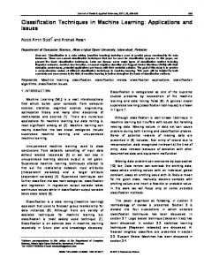
invented. Indeed, new science areas keep appearing, bringing with them a need for new mathematical notation. Quantum mechanics, for example, defined a new use of < and | to denote quantum states. The capital Greek letter Σ does not always denote a summation. The symbol < represents a comparison between numbers in 1 < 2, can be used as a kind of bracket in hx, yi, or in the definition of some mathematical objects in (C, 1.5 small We tried to train a single classifier based on all features for the symbol classification. When we analysed the results, we noticed that most classification errors correspond to the symbols which have little, if any, context. This leads us to building one classifier corresponding to each piece of context. On Figure 4.5, we represent the data for superscripted symbols in the space (EH,ED) (see previous section for explanations).

Figure 4.5: Data for superscripted symbols

The data points can already be clustered using these features. If we also consider the class of the superscript (ECLASS), there is almost no overlap. Two conclusions can be drawn: • the context appears to help the symbol recognition, and • a good classification should result from the separation of the classifiers according to which part of the context they represent. We have to note that this analysis considers the parameters to be right, especially regarding symbols’ classes (e.g. ECLASS, or P CLASS) and the relationships. In the

4.2. DESIGN OF THE SYSTEM

49

actual classification, some errors might result from mistakes in the symbol classification step, or in the structure recognition.

4.2

Design of the System

The design of the system includes different choices: • the way the data (from input to output) is represented • the way the components are associated to build the multi-classifiers • the values of the parameters and thresholds • the functionalities we want the system to have, other than the simple recognition of expressions • the way we want to display the information to the user In Section 4.2.1, we explain how we represent the data. Section 4.2.2 presents the design of the classifiers and their association. In Section 4.2.3, we present the design of some additional functionalities of the proposed system. Finally, in Section 4.2.4, we introduce the design of the user interface.

4.2.1

Representation of the Data

During the process, the form of the data changes. Indeed, the input is a binary image, and the output should be an interpretation of the expression. The different steps of the recognition have been identified. We must decide how to represent the data at each stage. In this part, we will present the data representation in a chronological order, starting with the form of the input, and finishing with the form of the output, as summed up on Figure 4.6.

Figure 4.6: Data Representation along the Pipeline

The input: a binary image

50

CHAPTER 4. DESIGN

We chose to take binary images (or bitmap) as inputs of the system. It represents the context in which mathematical formula recognition is needed. It corresponds to the case in which we have a printed (or handwritten) document which contains a formula that we want to extract to obtain an electronic form, which can later be reused. A binary image is merely a sequence of bits, which convey an information to the human eye when they are displayed in a visual form (an image). The information a computer gets by simply looking at the sequence is however limited. This is why we transform this data, by segmenting the image. Result of the segmentation: a list of bounding boxes The segmentation algorithm reads the image and extract connected components from it (see the ’Presentation of the Algorithms’ section). From the connected components found, we only keep the bounding boxes. This is indeed the simplest way to represent the layout of the expression. Each item in the list of bounding boxes is in the form xmin , xmax , ymin , ymax . In other words, it is the left, right, top and bottom bounds of each box. A list of symbols when the expression is created The list of bounding boxes is used to create the initial representation of the expression, which is merely a list of symbols. The structure of the expression is presented on Figure 4.7.

Figure 4.7: Representation of an Expression

The ’Symbol’ entity represents the symbol only, out of its context. It is created from the coordinates of the bounding box. It contains information about the size and position of the symbol. The ’Context’ entity represents the symbol in its context. It can be linked to other symbols (Contexts) such as the parent of the symbol or its children. It also contains the relationship the symbol has with its parent, and the confidence values on the class of symbol and on the relationship.


51

The ’Expression’ entity is made of the list of symbols (Contexts). The creation of the expression builds a ’Symbol’ object for each bounding box in the list, and create a ’Context’ for each symbol. All contexts are stored in a list, which is the ’Expression’. The classification builds a tree The aim of the classification and the recognition is to find the relationships between symbols, and to find the symbols classes. This can be seen as linking symbols together, and adding information to the existing structure. From the initial list, a tree is created. Similar tree representations can be found in the literature (such as [21, 9, 28]). Each node corresponds to a context. As explained before, the information contained in a node is: • the corresponding symbol • the relationship with its parent • the regions where children should be found • the distributions of confidence values over the possible symbol classes, for each classifier (see next part) • the distribution of confidence values over the possible relationships with the parent Each child of a node corresponds to a child of the symbol represented by this node. There is also a backward linking to access the parent of the symbol. The tree representation is summed up on Figure 4.8. A partial example of such a tree is showed on Figure 4.9, for the expression ba pn . Exporting the results as an XML document Once the classification is done, we want to be able to save the result. There are several goals for that. First, it could be used by another program to finish the recognition. Indeed, we classify symbols and recognize the structure, but some work must still be done. For example, the recognition of each symbol, or even the equivalent of the lexical pass described in [28]. The result saved can also be reused by the program, to load the interpretation of a formula for example. We have chosen an XML form, because it translates well the nested structure of a mathematical expression. Moreover, an XML document is a tree structure, like our expression representation is. The document must contain the important information: • The expression, its width and height • The symbols, their class, relationship, bounds, and the confidence values for each class and relationship

52

CHAPTER 4. DESIGN

Figure 4.8: Expression Tree

Figure 4.9: Example of an expression tree

The root of the document is the expression node. It has only one child which is the representation of the root of the expression tree. It is a symbol node. A symbol node has three attributes:


53

• The id attributed in the creation of the expression • The symbol class id • The relationship id The symbol id is used when the XML interpretation is loaded by the program, in order to be able to identify the correspondence between a node in the expression and a node in the document. It has several children: • A bounding box node, which contains the coordinates • A symbol class node, which contains the confidence values for each class • A relationship node, which contains the confidence values for each relationship • A symbol node for each child An example is shown on Figure 4.10.

Figure 4.10: Expression Interpretation in XML

4.2.2

Practical Design of the Classifiers

The part of the system that actually recognizes the expression is made of classifiers, such as neural networks, or fuzzy systems. The system is an association of these different entities. Each component is designed for a particular role. We have to choose the best suited system to represent it, and adjust the parameters, define how it will be trained for example, or also which kind of results is expected. We also have to choose how these

54

CHAPTER 4. DESIGN

different components are associated together, how their outputs are mixed to obtain the final result. The system is made of two parts, one for each task. We will present first the Symbol Classifier (SC), and then the Relationship Classifier (RC). 4.2.2.1

Symbol Classifier

Its aim is to classify the symbols into one of the four classes ’small’, ’descending’, ’ascending’, ’variable range’. It would not be appropriate to give a straight answer because we consider only the bounding boxes. Rather, we should return the confidence values for the symbol to be in each class. According to our plan, we want to consider the context of the symbols to classify them. We will use a system composed of several classifiers. Indeed, having only one classifier poses two problems: • At the first step of our algorithm, we perform a first symbol classification when no context is available, so we have to have a classifier which does not take the context into account. • All symbols have not the same amount of context. Some symbols might have very little context. For instance, in ba pn , n only have a parent, but no child. If we have a single classifier, the absence of context may be understood as an important information, when it is rather a lack of information. We will first present and justify the choice of the multi-classifier. Then, we will explain how the parameters are chosen, and how the components are trained. Form of the classifier The system chosen is a multi-classifier which can be adapted to each symbol, given its context. The different classifiers each returns a set of confidence values which are then merged together. The system is summarized on Figure 4.11. The output is a mix of the ratio based classifier, the parent based classifier, and the children based classifier. This last one is made of five classifiers, one per possible child. In the following, we will present each classifier briefly. Then we will give a justification of the general form. Children based Classifier. The children based classifier is made of five artificial neural networks, one for each possible child. The 4 inputs of each classifier are • the class of the child, • its relative vertical position, • its relative horizontal position, and • relative size to the parent.


55

Figure 4.11: The Symbol Classifier Parent based Classifier. The parent based classifier looks at the relative position and size of the symbol to its parent. It also takes into account the parent’s class, and the kind of relationship (e.g. subscript) the symbol has with its parent. It is also an artificial neural network. Ratio based Classifier. The ratio based classifier allows to classify the symbol regardless of its context, using only the bounding box information. It is particularly useful for the first step of the classification: the rough symbol classification. Indeed, at this stage, no parenting is done, and no relationship is identified. We use a Bayesian inference system. We assume that the ratio (or shape of the bounding box) is a consequence of the symbol class. Indeed, symbols of the same class are likely to have a similar shape. For example, ’small’ symbols, such as ’a’, ’n’ or ’m’ generally have a ratio width/height equal or higher than 1. Justification of the form The whole classifier is divided into several classifiers, associated as presented above, because: • The context is a variable amount of information, which must be handled in a particular way (see next paragraph). • It is crucial to give different importance to different pieces of information. For example, if we had a single classifier, we would not have very much control on the predominance of the ratio information over the class of a superscript for example.

56

CHAPTER 4. DESIGN

The ratio has a strong correlation with the symbol class, whereas the child class is not directly dependant on the symbol class. We clustered together the features which make sense only when they are taken together, e.g the information about the subscript is different from the one about superscript, and the information about the parent, the children and the ratio are different kinds of information. • The last reason was that we needed a component for the rough symbol classification, when no context is available Handling the lack of context The system is made for the classification of a symbol in a full context. However, in mathematical expressions, most symbols have an incomplete context. We thought of two ways of handling this lack of context. First, we can ignore the classifiers which correspond to a non-existing context. The system for a symbol which has no parent, and only a superscript, would then be as presented on Figure 4.12.

Figure 4.12: Context-Adapted Symbol Classifier

In this approach, the symbol is classified regardless of the amount of context. In the previous example, the result of the children classifier only considers the superscript based classification. It amounts to saying that the other child based classifiers would have yielded the same result as the superscript based one. However, the missing context corresponds to a lack of information. This should be reflected in the final confidence values. Therefore, we decided that the corresponding classifiers should return a ’full-uncertainty’ result, an uniform distribution of confidence over the classes. It has a smoothing effect when the results are merged. Parameters and Training of the Components The ratio-based classifier is a simple Bayesian inference. However, the usual Bayesian inference takes into account the prior probability of each class. It is usually computed by calculating the frequency of each class in the data set. In our data set we have more


57

Table 4.5: Parameters of Parameters Learning rate: 0.3 Momentum: 0.2 Epochs: 500 Inline child based Learning rate: 0.3 Momentum: 0.2 Epochs: 500 Other child based Learning rate: 0.3 Momentum: 0.2 Epochs: 500 Classifier Parent-based

the Symbol Classifiers Number of examples Accuracy 2981 72.2%

1553

70%

About 800

About 98%

ascending symbols, but it does not mean that ascending symbols occur more often in equations. We modified the inference by giving each class the same prior, so we have: P (class | ratio) =

P (ratio | class) ×α P (ratio)

where α is a normalizing constant. This classifier is built and trained with Weka. It only classifies well 251 out of 372 examples (67.5%). It can be due to two facts. As we saw in the analysis of data, there are severe overlaps in the distribution of ratios for each class. Besides, this training is done considering the prior on symbol class, which will be removed in a later step, within the classification algorithm. The neural networks are trained with a 10-fold cross validation. The parameters are summarized in Table 4.5. The percentage of well-classified examples is also shown. They all have 7 inputs (3 numerical for parameters (H-, D- and V -like)2 and 4 binary for the class of the parent or child (P CLASS, LCLASS, and so on)). A low accuracy is not always a problem, because (a) the classifiers will be associated, and some mistakes will be corrected by the other classifiers, and (b) the confidence values are more important than the classification in this context. For the final classification, the outputs of each classifier are mixed. The confidence values are weighted sums of the different outputs. Final = α× Ratio-based + β× Parent-based + γ× Children-based The children-based classifier is the most important, because it contains the most interesting parts of the context. It is given the highest weight (γ = 0.55). The parent is a different part of the context, because the relative position with respect to the parent is for example more due to the parent class than to the symbol class. It is then given a smaller weight (β = 0.10). Therefore, is really has an effect when the confidence of this classifier is very high. The ratio is a direct consequence of the class, but as we saw, is often not sufficient for a good classification. The weight is accordingly moderate (α = 0.35). The children-based classifier’s output is the average of the outputs of all child-based classifiers, because there is no reason to give an advantage to one particular relationship. 2

for the definition of these parameters, see page 58

58

CHAPTER 4. DESIGN

4.2.2.2

Relationship Classifier

The aim of this classifier is to determine, given two symbols, which is the most likely relationship between them. Similarly to the symbol classifier, we return confidence values for each class rather than a crisp classification. However, we aim at higher confidence than for the symbol classification, because the relationship classifier is also used for the parenting. The relationship classification assumes that we know the class of the symbols involved, even if this information is wrong. It uses this class information, along with the relative size and position of the symbol to deduce the relationship. The components of the classifier are a neural network, fuzzy regions and fuzzy baselines. We will present the general form of this part of the system, describe the different components, and explain the choice of the parameters. Form of the Classifier The classifier is made of several independent parts, each of which giving confidence values on the relationships. These results are merged to give the final answer, which can then be compared to the thresholds. The system is presented on Figure 4.13.

Figure 4.13: The Relationship Classifier

A Neural Network The central part is a neural network. It has been trained by the data set to efficiently recognize the relationship between two given symbols. The inputs are parameters inspired by [25, 2]. These are: • H - the relative size of the child to its parent: H = • D - the relative vertical position of the child: D =

hp hc yp − yc hp


• V - the relative horizontal position of the child: V =

59 xmaxp − xminc wp

where the indices p and c stand for ’parent’ and ’child’, h is the height, w is the width, y is the vertical centre of the bounding box, and xmin and xmax are the left and right bounds. V is not used by Aly et al., and has been defined for this project, to facilitate the differentiation of subscript and under, and of superscript and upper. The idea is that, while H and D can be very similar for the ’subscript’ and ’under’ relationships, V can make the difference, being positive for ’under’ and negative for ’subscript’. These parameters have been proved by Aly et al. [2] to be efficient. However, they use normalized bounding boxes to calculate them. To do so, they have to know the identity or class of the symbol, and they add a virtual ascender (to the ’small’ and ’descending’ symbols) and a virtual descender (to the ’small’ and ’ascending’ symbols). We do not want to modify the bounding boxes, and we want to keep as much uncertainty as possible. Instead of normalizing bounding boxes, we also set the parent and child classes as inputs of the network. Fuzzy Regions The use of fuzzy regions for the structure recognition was influenced by the work of Zhang et al. in [29]. The aim of this system is to assist the neural network to classify the relationships, but also to tell when the symbols are not in a relationship, which the former network cannot do. It is particularly useful for the parenting task. The fuzzy regions are used for all relationships except ’inline’, where fuzzy baselines are used instead. They consist of a crisp region, and a fuzzy area. Examples of how fuzzy regions are build can be seen on Figure 4.14.

Figure 4.14: The Fuzzy Regions

60

CHAPTER 4. DESIGN

To evaluate the confidence for a child symbol to be in a particular relationship with a possible parent symbol, we compute the membership value for the center of the left bound of the child in the corresponding parent’s fuzzy region, as we can see on Figure 4.15.

Figure 4.15: Membership Values Computation

Fuzzy Baselines Unlike the other children, an inline child is not necessarily close to its parent. It makes the use of regions more difficult. However, by definition, an inline child is on the same line as its parent. Baselines are the lines where symbols are written. The position of the baseline of a symbol mainly depends on its class, as shown on Figure 4.16. This relative position could be learnt if we had a data set with this information. Because of the limitations on time, we decided to calculate it by hand. In fact, our project focuses on printed Latex formulae, where the position of the baseline is the same for all symbols of the same class. These positions are presented in Table 4.6, expressed relatively to the symbol’s height.

Figure 4.16: Position of the Baseline

Because we produce a flexible solution, we handle the possible variation of the writing line by considering fuzzy baselines. For a pair parent/child of symbols, we proceed as follows. First, we calculate the baseline of the parent, given its class. Then, we look at the possible baselines of the child, and calculate a confidence score based on the distance from the parent baseline and on the confidence of the child class.


Table 4.6: Class small descending ascending variable range

61

Baseline Positions % of the symbol’s height 100 70 100 75

The width of the fuzzy baseline depends on the size of the symbol, but the general shape is presented on Figure 4.17. It shows the confidence as a function of the distance between the baselines compared, in pixels.

Figure 4.17: Baseline Score

Use of the Relationship Classifier The relationship classifier is used for the identification of relationships, but also for the parenting task. The classification does not involve a simple mixing of the different classifiers, as in the symbol classification. The algorithm for this task will be described later. For the parenting task, an extra classifier is defined. The possible-child classifier, which, given two symbols, tells if the second can be a non-inline child of the first one. This decision tree takes into account the relative size and position of these symbols, as well as their classes. When we try to find the relationship of a symbol, we first check if it can be on the same line as another symbol. We combine the confidence value given by the neural network, the baseline score and the confidence of not being a non-inline child, considering each possible parent. If no inline parent is found, we check if the symbol can be the child of another symbol, using the corresponding confidence values for the neural network, the fuzzy regions and the possible-child classifier. Parameters and Training of the Components Relationship Classifier To train the neural network, we only consider the examples in the data set which correspond to symbols having a parent. The neural network has actually 11 inputs. Three are

62

CHAPTER 4. DESIGN

numerical (H, D and V ), and eight are binary (P CLASS = 1 . . . 4, CLASS = 1 . . . 4). We have 8 neurons in the hidden layer, and 5 outputs, one for each relationship. For the training, the learning rate is 0.2, the momentum is 0.2 and the number of epochs is 500. In the training set, there are ten times more inline, superscript and subscript relationships than upper and under. Thus, we used a cost matrix to train the network, such that there is no preference in the final classification for the first three relationships. 2977 of the 2981 training examples are correctly classified by the final network, but we have to remember that this network cannot tell if two symbols are not in a relationship. Possible-Child Classifier The possible-child classifier is a decision tree. It is trained with 3875 pairs of symbols, either inline or not in a direct relationship, and 3463 pairs of symbols in one of the four non-inline relationships, using the J48 algorithm. It has been trained with a minimum number of objects per leaf set to 30. The training with a 10-fold cross-validation reached 95.9% of correctly classified instances. Fuzzy Baselines The fuzzy baselines are built by hand from the observed relative position of the baseline for each class. They are used to calculate a baseline score, which have two levels of fuzziness. The first one is based on the distance of the baseline to the parent’s baseline. The score is computed as follows: α b1 = α+d where d is the distance and α is a parameter based on the height of the symbol (α = 16% × H). Indeed, if the fuzziness was independent from the size of the symbol, small symbols would have a higher risk to be misclassified as inline. The second level of fuzziness is the uncertainty on the symbol class. The score b1 is multiplied by the confidence on the symbol class to obtain the final baseline score. Fuzzy Regions The fuzzy regions are defined according to some statistics regarding the data set. For each class, and each relationships, we retrieve the mean and standard deviation of the parameters D and V . The means allow to define the center of the crisp regions, and the standard deviations their width and height. If X and σX are the mean and the standard deviation of X, given the definitions: yp − yc D= hp xmaxp − xminc wp we define the coordinates of the crisp region: V =

xmin = x − w ∗ (V + σV ) xmax = x − w ∗ (V − σV ) ymin = m − h ∗ (D + σD ) ymax = m − h ∗ (D − σD )


63

where x is the right bound of the symbol, w and h its width and height, and m its vertical center. The margins, or fuzzy areas, are computed using the relative size of the symbols, represented by the parameter H. The vertical (top and bottom) and horizontal (left and right) margins are calculated as follows: hmarg = vmarg =

1 h ( − hcrisp ) 2 Hmin 1 h ( − wcrisp ) 2 H

hp , h and w are the height and width of the symbol, and hcrisp hc those of the crisp regions. This is summarized on Figure 4.18.

where H is the parameter and wcrisp

Figure 4.18: Building the Fuzzy Regions

For the relationships upper and under, the calculations are different, because the training set does not represent the complex reality. Indeed, in the training set, there is always at most one symbol above and one under. Unlike superscripts and subscripts, the horizontal positions of these children change when there is more than one symbol. The regions’ vertical bounds are still defined as before. The horizontal bounds are: • Left bound: for the crisp region identical to the left bound of the symbol’s bounding box ; for the fuzzy region, the left bound of the symbol minus 15% of the symbol width • Right bound: for the crisp region, calculated as before, for the fuzzy region, add 15% of the symbol’s width Finally, the training set does not have upper and under relationships for small, descending and ascending symbols, nor subscripts and superscripts for variable range symbols.

64

CHAPTER 4. DESIGN

Therefore, we build the corresponding regions with the parameters relative to other symbol classes. For example, the parameters of variable range symbols are used to build the fuzzy region ’upper’ of a small symbol. Associating the Classifiers When the algorithm parents symbols and labels relationships, the different classifiers are used, and a weighted sum of the values they return is calculated. A different treatment is applied depending on whether the relationship is inline or not. The weighted sum is then compared to a threshold. In this project, we found that 0.55 was an acceptable threshold, i.e. giving good results. The coefficients for the inline relationship are • Relationship Classifier: 1, low because it cannot tell whether the considered symbols are in a relationship • Possible-Child Classifier: 1, low because the answer ’No’ of this classifier can mean either inline or no relationship • Fuzzy Regions: 0, because there is no fuzzy region for this relationship • Fuzzy Baseline: 4 It means that a low baseline score can be compensated by a high certainty of the other classifiers, but the other classifiers cannot alone classify an inline relationship. The weighted sum is divided by 1+1+4=6 to be compared to the threshold. The coefficients for the other relationships are • Relationship Classifier: 1 (for the corresponding output) for the same reasons as before. • Possible-Child Classifier: 2, higher because the answer ’Yes’ means that the pair of symbols are in a non-inline relationship • Fuzzy Regions: 4 • Fuzzy Baseline: 0 The fuzzy regions are selective, but a low confidence value can be compensated by a high confidence of the other classifiers.

4.2.3

Functionalities of the System

We do not only aim at a mathematical formula recognizer. As designer of this intelligent system, we want to be able to test it. This adds some functionalities to the system. In this part, we will present briefly some of these additional functionalities, that we felt important for the system to have.


65

The list of these functionalities is: • Manually selecting of removing the parent of a symbol • Manually labelling symbols and relationships • Classifying symbols only • Classifying relationships only • Viewing possible relationships between any two symbols • Handling several expressions • Exporting the interpretations to create a test set • Comparing the recognition with the actual interpretation Manual selection and removal of symbol’s parent It can be useful to parent symbols by hand. For instance, when we create a test set, we need to link symbols together in order to label the relationship. When we want to test the relationship classifier independently from the parenting algorithm, it is also useful to parent symbols by hand. Implementing the possibility of clicking on a symbol and change its properties intuitively is a key part of the GUI. Manual labelling of symbols and relationship The other feature for the design of a test set is the possibility of manually label symbol classes and relationships. When a symbol is selected, we should have the option of selecting its class. If it has a defined parent, we can also select the relationship. By doing so, the context of the symbol is updated. The data structure used is the same as the one used by the classifier. Thus, we can for example label relationships and test the symbol classifier only. Classification of the symbols only or the relationships only The system is complex, and made of several classifiers. Our classification algorithm tries to recognize the expression through an iterative process, where the symbol classification and the structure recognition constrain each other. It is important to be able to test each part independently. Making the classification of the relationships only (or of the symbols only) possible allows to assume that the symbol classification and the parenting (or the context of the symbol) is known, and to test how a particular part of the system performs given this information. Relationship table

66

CHAPTER 4. DESIGN

Testing the parenting only is more difficult. Indeed, in our algorithm, the parenting is done at the same time as the relationship classification (see next section ’Presentation of the Algorithms’). More particularly, we parent symbols according to scores that are based on the relationship classification. To analyse the parenting, understand errors, and adjust scores thresholds, we need to display a ’relationship table’. To build it, we use the fact that in most cases, the parent is on the left of its children. For each symbol, we classify the relationship it might have with every symbol which is on its right side. An example of this table is shown on Figure 4.19.

Figure 4.19: Relationship Table

The table is only built for analysing and designing the system. In the actual parenting algorithm, we do not need such a complexity ( O(N 2 ) classifications, if N is the number of symbols). Processing several expressions at the same time Opening an input file, processing it, analysing the results and closing it is a long operation, especially when we want to handle a test set. In this case, it is also interesting to see the performance on the whole set rather than on each instance in the set individually. Therefore, we allow the system to open several files in once, or to read several expressions in a Latex file. In the workspace, we then have a list of expressions rather than only one. The particular usefulness for the test set building is explained in the next paragraph. Creation of a test set The system is built by training each classifier individually. We need a big data set, which was built automatically. This process cannot be applied to the creation of a test set. Indeed, we have to test the whole system. In particular, the parenting cannot be tested with a database composed of symbol instances. Therefore, we implemented the possibility to let the designer build a test set. To do so, we can open several input expressions,


67

manually parent the symbols and classify them and their relationships. Then, the test set should be stored as an XML file, and loaded again later to compare the recognition of the expressions with it. Testing the system To evaluate how good the system is, we have to test is. That means, we have to compare its results with expected results, which are stored in a test set. To test the system, we open a set of expressions, the same as the one used to create the test set. Then, we ask the system to recognize these expressions. We obtain the symbols classes, parents and relationships. We then read the XML test set. We can finally compare the lists of symbols in the recognized expression and in the expression from the test set. The comparison of two expressions returns a set of performance features. It includes the following information: • Percentage of errors on symbol class • Percentage of errors on relationship class • Percentage of parenting error (when symbols are associated with the wrong parent) • Symbol correctness score • Relationship correctness score The correctness score illustrate how confident the system is on the right class or relationship. These scores are explained in the chapter ’Results and Evaluation’.

4.2.4

Integration of the Classifiers in an User-Friendly Interface

It is good to have a code which can perform many actions. However, it is a waste of time if we have to re-launch the program for every action we want to perform, and every time we change the input. Therefore, we integrated the system in a graphical interface. It is a benefit in time for two reasons. First, we have buttons that we can click for each action, and in particular we can test several inputs by opening several files without closing and starting the program again. Second, when something does not work, we can spot the origin of that dysfunction by looking at all the information displayed. We include in this ’user-friendly’ part of the system a set of functionalities, and a set of features. To have more details, report to the ’Implementation’ chapter. 4.2.4.1

Functionalities of the Interface

Besides providing buttons and menus to execute the functionalities described before, the interface should have two main functionalities: • Display all relevant information, as well as the recognition results, and • Allow an easy setting of inputs. Display information and results

68

CHAPTER 4. DESIGN

The goal is to give the user and the designer of the system the important information about the expression and the recognition. The display should be organised, intuitive, and easy to use. This is described in more details in the following part - ’Features of the interface’. Set inputs Another important function is to make the setting of inputs quick and easy. Due to our requirements, we should be able to load one or several inputs. We have implemented four ways of setting inputs: • By loading binary images, • By entering a LATEXcommand, • By reading a LATEXfile, • By reading an XML file. When we click on an image file in the workspace, we can choose to open the image. We can also click on an ’Open’ menu. We have designed a window with a text field, where the user can type a Latex formula. It is then automatically converted into an image. We have also implemented a Latex parser. It reads a Latex file, and retrieve the text between the tags ’begin{equation}’ and ’end{equation}’. Each one of them is then converted into an image. For each of these methods, the images are then segmented, and the representations of symbols and expressions are created before it is included in the interface, to be used. The last possibility is to read an XML file. The document should be in the form presented in the section about data representation, in the paragraph ’Exporting the results’. In the document, the bounding box information allows us to display the layout of the expression. The XML file should also contain the interpretation of the formula. 4.2.4.2

Features of the Interface

An organized visual display of the information is often easier to understand than a text output in a console. The aim of an interface is to provide this display. The set of features can be divided into five major parts: • Display of the input • Display of the input’s properties • Display of the classifiers outputs • Display of the results • Display of the file system We will present these features and why they are interesting. Display of the input


69

The input display allows to see the image input - the mathematical expression - and its segmentation. We can check if the segmentation is right. It shows the bounding boxes of symbols. We should also have the possibility of clicking on a symbol to display its information (e.g. width, height, class) and the result of its classification. We should also be able to show all the visual information about this expression. For example, we can display the baselines with their confidence, the links between symbols, corresponding to the parenting, or the regions associated with the symbols. Finally, we want to be able to process several inputs at the same time. Thus, the interface contains several layers, one for each expression. Menus are provided to jump from one input to the other. Display of the input’s properties When we click on a symbol, it would be interesting to see its features, so we can for example understand the input of the classifiers and the possible mistakes. Display of the classifiers outputs Each part of the multi-classifier system, presented before, returns confidence values on the symbol class and relationship with the parent. The outputs are merged to give the final result. It is interesting to show the output of every part, to see how they perform. For each part, the output is presented in the form of an histogram, showing the confidence value for each class. Display of the results When we have recognized an expression, it is interesting to show the results, in terms of the goodness of the interpretation. It is used in two situations. For the mere recognition of an input, we show the global confidence on the symbol recognition, on the relationship recognition, and of the whole recognition. When we test the system, that is when we compare the actual interpretations with the expected ones, we show a correctness score, or accuracy. For the latter case, we plot the results. We can choose which score to display (e.g. symbol correctness score as a function of the number of symbols). It gives more information than displaying simple text. We also have a window to output the results in a textual form, to show the exact figures. Display of the file system The use of the system involves opening input images, loading classifiers, reading tex files, or importing XML interpretations. To make that process easier and faster, we set a sort of workspace. A window displays the file system of the computer, highlights files that can be used by the program, and shows the possible actions available when a file is clicked.

70

CHAPTER 4. DESIGN

4.3

Presentation of the Algorithms

We cannot present all algorithms used in the project, but the most interesting ones can be found in the appendix ’Algorithms’. In this section, we will present three algorithms. The first one is the first of the process - the segmentation algorithm. Then, the most important algorithm, used for the recognition, is explained. Finally, we show how we can export the results, or manually labelled interpretation, to create a test set for example.

4.3.1

Image Segmentation

For the recognition, we assume that we know the bounding boxes of the symbols. These are the inputs of our system. To build a data set, or to construct a test set for the system, it is more convenient to have a segmentation algorithm, so that the inputs are calculated directly from images. There are very efficient segmentation algorithms existing, but we chose a very simple one. We make the strong assumption that all printed symbols are connected. This is not the case for i, j, =, and so on, but we will ignore them for the sake of simplicity. The chosen algorithm is a two-pass algorithm for the detection of connected components. The Algorithm Two-pass means that we go only twice through the image. The idea is to label the connected components present in a binary image, with a different label for each component. In the first pass, we label the image, and we record the equivalences between labels. To do so, we proceed as follow, for each pixel: 1. if it is a background pixel, move to the next pixel 2. otherwise, look at the labels of the surrounding (already labelled) pixels 3. if there is no label around, mark the pixel with a new label 4. otherwise, mark the pixel with the lowest label, and record the equivalence with the adjacent labels. At the end of the first pass, every foreground pixel has a label. Several pixels in the same component may have a different label, but they are all equivalent to the lowest label in that component. In the second pass, we update every pixel’s label with the equivalent label. Normally, after this pass, there is only one label in each component. The goal is to retrieve the bounding boxes, so during the second pass, we also record the minimum and maximum coordinates in both x and y directions. The algorithm returns a list of bounding boxes. We can see how the algorithm works on Figure 4.20.

4.3.2

The Recognition

The classification algorithm, or recognition algorithm, is the most important of the system. It consists of two parts. First, the symbol classification only creates the neural networks inputs and merge their outputs, for each symbol. Then, the structure recognition

4.3. PRESENTATION OF THE ALGORITHMS

71

Figure 4.20: Segmentation Algorithm algorithm is more complicated, because it computes two tasks. If finds the parent of each symbol, and the relationship between them. In the following, we will describe the different steps of the recognition. 4.3.2.1

Rough Symbol Classification

The first step is the classification of every symbol based on the ratio width/height. The Bayesian Network returns confidence values, which are divided by the prior on symbol classes, to obtain the scores described previously. The algorithm is summarized on Figure 4.21. 4.3.2.2


We tried to design a fast structure recognition based on machine learning techniques. We wanted to limit the backtracking and the recursion for the parenting task and the identification of relationship. Comparing each possible pair of symbols is out of the question. Our algorithm does the parenting in one pass, with a limited backtracking. Inline relationships are more difficult to find because the symbols involved can be far apart. Other relationships involve symbols close to each other. Therefore, we first try to see if a symbol is inline with another before checking for other relationships. Moreover, a symbol can be inline with several others, whereas it can only be the subscript of one. Given one symbol, we first check whether it is an inline child. We compute the score, as explained before, considering only the last symbol of each baseline as possible parents. The baselines are considered from the most dominant to the most nested. If one score

72

CHAPTER 4. DESIGN

Figure 4.21: Rough Symbol Classification is higher than the threshold, we stop the search and do the parenting. The list of last symbols for each baseline is updated. If no inline parent is found, we browse the stack of last symbols seen, and we check whether the considered symbol can be a child of one of these last symbols. Since a noninline child is often close to its parent, the parent is likely not to be far in the stack. Hence the backtracking is limited. We also remember the most likely parent and relationship. Thus, if no confidence is higher than the threshold, we check if there is no child for the most likely parent in the most likely relationship, and we can parent the symbol. Otherwise, the symbol is left without a parent. The complexity of the backtracking is in the worst case 2 × R × C where: • R is the number of non-inline relationships, which also corresponds to the maximum number of nested baselines created from one symbol • C is the complexity, so the number of last symbols on baselines is lower than R × C, as is the number of possible children for these last symbols. The algorithm has just one pass, so the total complexity is 2RCN in the worst case. Even if RC > N , not every symbol has a child for each relationship, so in practice the complexity is less than N 2 . The algorithm is explained on Figure 4.22, and an example is shown on Figure 4.23. 4.3.2.3

Symbol Classification using Context

For the symbol classification using context, the inputs of the networks corresponding to each existing piece of context are computed, and the outputs of the networks are collected. The final confidence values are calculated as explained before, and the class is inferred. This algorithm is summarized on Figure 4.24.


73

Figure 4.22: Structure Recognition Algorithm

Figure 4.23: Structure Recognition Example (fon n in Abn ) 4.3.2.4

The Iterations

The iterative process is initialized with the rough classification. Then, at each iteration, three operations are performed. First, all existing relationships are undone. Then, the structure is recognized, and finally, the symbols are classified. This is shown on Figure 4.25.

74

CHAPTER 4. DESIGN

Figure 4.24: Symbol Classification Algorithm

Figure 4.25: The Iterative Algorithm

4.3.3

Exporting the Results

The last step of the recognition is exporting the results. In fact, we do not perform the whole recognition, and exporting the results could allow another program to read the interpretation and perform more actions, such as the symbol recognition. Besides, it allows to save a test set, so we can evaluate the system later. The algorithm transforms the expression tree as it is implemented in the system into an XML tree containing enough information to store the interpretation. The process is


75

recursive. Considering a symbol, its properties (bounding boxes, classification) are stored in nodes. The children symbol nodes are created recursively. Indeed, each child correspond to a nested expression and can be processed the same way.

76

CHAPTER 4. DESIGN

Chapter 5

Implementation The implementation is the actual realization of the designed system. It consists of the design and the writing of a program which can be run on a computer, to perform the recognition task. It should also represent the data in an efficient way, contain the different functionalities described before, and present the whole system in a user-friendly interface. The translation of these functionalities into use-case diagrams can be found in the ’Implementation’ appendix. We chose an object-oriented approach because it translates well the division of the whole system into different components. Indeed, we can identify: • a core part, which represents the expression and perform the classification • an input/output part to avoid redoing always the same things • a graphical user interface (GUI) The key part for implementing an object-oriented system is to model it. For instance, we have to divide it into different classes, each of which having a particular role. The proposed implementation uses frameworks (Weka, JDOM and JLatexMath) and a database, implemented with MS Access. The developed system is divided into several packages, presented on Figure 5.1, and explained in the appendix. Section 5.1 explains the implementation of the expressions and the classifiers. Section 5.2 breifly presents the implementation of some additional functionalities. Section 5.3 introduces the implementation of the GUI. Section 5.4 presents the objects implementated for the structure recognition. More details can be found in Appendix A.

5.1

Implementation of the Expressions and Classifiers

The core of the system is the recognition mathematical expressions. We presented previously the representation of the data and the form of the classifiers. In this part, we will enter in more details about how this representation is implemented. We will present the different classes, their association, and their role.

5.1.1

Implementation of the Expressions

As explained before, the expressions are represented in terms of the symbols they contain, considered in their context. It corresponds the five classes of objects, presented in the 77

78

CHAPTER 5. IMPLEMENTATION

Figure 5.1: Package Diagram class diagram on Figure 5.2. These classes constitute the content of the package ’core::me’. We represented only the most useful methods. Most of them are self-explanatory. The details are exposed in Appendix A and in the API provided on the attached disk.

Figure 5.2: Expression Implementation

Class Symbol The objects in this class are very basic representations of symbols. In fact, they contain information about the symbol itself, out of any context. A Symbol object is created from the bounding box. It provides geometrical information such as the height, the width, the position, or the centre of the bounding box. The symbol id is especially useful when testing

5.1. IMPLEMENTATION OF THE EXPRESSIONS AND CLASSIFIERS

79

the system. Class SymbolClass A SymbolClass object represents the whole classification of a symbol. Therefore, it contains the output of all the classifiers involved in the classification, and the way they are mixed to yield the final confidence values. Class Relationship Similarly, a Relationship object represents the classification of the relationship existing between a parent and its child. It stores the output of the different classifiers, and the final confidences. Class Context An object in this class is referred to by the word ’symbol’ throughout the dissertation. Indeed, our approach not only recognizes the structure, but also uses it to find the class of symbol. Therefore, the context of the symbol is as important as the symbol itself. A Context object is a node in the final expression tree, since we can link it to other Context objects. As we explained, the node also contains a SymbolClass and a Relationship object. Its basic role is to represent the result of the recognition. Class Expression The Expression object allows to see the expression more globally. It is basically a list of all symbols, sorted from the leftmost to the rightmost symbol. It provides an easy way of retrieving the information regarding the whole expression, such as its interpretation, its dimensions, the leftmost symbol ( root of the tree structure after the recognition), or to apply some action to all symbols (e.g., for the symbol classification).

5.1.2

Implementation of the Classifiers

The classifiers are used to recognize the structure. First, the trained classifiers, the neural networks for example, are all stored in one independent class, whereas fuzzy regions are defined with respect to a symbol. Fuzzy baselines do not correspond to a particular class. Finally, the structure recognition is performed by the RelationshipFinder class. 5.1.2.1

Trained classifiers

All classifiers which need a training from the data sets are trained, saved, imported, stored and used within a single class, Classifiers. It adapts the Weka framework to the needs of our project. The attributes of this objects are the classifiers and the data structures needed to build an instance that can be read by the corresponding classifiers. They are summarized in Table 5.1. This class implements three kinds of methods: • save and read methods use the serialisation provided by Weka, to avoid training the classifiers every time the program is executed.

80


Classifier SCA SCB

SCC1..5

RC

YN

Table 5.1: Implementation of the classifiers Class Description Data Structure weka.classifiers. Ratio-based symbol dataStructSCA bayes.BayesNet classifier weka.classifiers. Parent-based symbol dataStructSCB function. classifier MultiLayerPerceptron weka.classifiers. Children-based symbol dataStructSCC1..5 function. classifiers MultiLayerPerceptron weka.classifiers. Relationship classifier dataStructRC meta. CostSensitiveClassifier weka.classifiers. Possible not-inline clas- dataStructYNC tree.J48 sifier

• train methods do the training of the classifiers, with cross-validation, and build the data structures. • classify methods, such as getSymbolClassA( Context ), allow the classification of a symbol or a relationship by a single classifier, and returns a distribution of confidence values. This is summarized on Figure 5.3.

Figure 5.3: Classifiers Class

5.1. IMPLEMENTATION OF THE EXPRESSIONS AND CLASSIFIERS

5.1.2.2

81

Fuzzy Regions

An overview of the classes of objects related to fuzzy regions is shown on the class diagram on Figure 5.4.

Figure 5.4: Fuzzy Regions Implementation

Each fuzzy region is represented by the class FuzzyRegion. The membership() method calculates the membership value of a point in this region. Four regions (one per possible relationship) are grouped into a FuzzyRegions object, to represent all fuzzy regions associated with an object. A second level of fuzziness is introduced by considering the uncertainty on the symbol class. Each symbol is associated with a ContextFuzzyRegions object, which contains four sets (for the four possible symbol classes) of fuzzy regions. These are objects of the classes SmallRegions, AscendingRegions and so on. The membership values are computed for each regions and each symbol class, and then summed up, weighted with the confidence of the corresponding symbol class. 5.1.2.3

Fuzzy Baselines

The baseline scores are computed as previously explained by the baselineScore(Context) method in the Context class. The argument is the parent symbol, and the method returns an array containing the calculated baseline scores, based on the distance of the symbol’s baseline to the parent baseline, for each symbol class. 5.1.2.4

Structure Recognizer

The structure recognition is performed by the object RelationshipFinder. It is associated with an Expression object, in which symbols are already classified. The method

82


parentAndRelate() implements the structure recognition algorithm. The details about the implementation of the algorithm can be found in section 5.4, and the code is presented in Appendix B.

5.1.3

Tools for the Analysis of the Classification Results

Two classes represent tools for the analysis of a classification, namely Interpretation and Statistics. The first one stores the information about the interpretation of an expression, that is, the global confidence score concerning symbol classes and relationships, the Latex equivalent of the expression, the XML document corresponding to the interpretation, and the validity of the expression. The goal of Statistics is to test the system. It stores information such as the percentage of symbol class, relationship or parenting error. It is used when we compare the actual expression recognition to the expected one, saved in XML format on the computer. More details about this class can be found in the next chapter ’Results and Evaluation’.

5.2

Additional Functionalities

Most functionalities, both crucial (e.g. the symbol classification) or annex (e.g. the visualisation of the results), are implemented by the classes presented before, or by the GUI (next section). In this section, we will briefly present three classes, which provide essential tools for building and using the system: LatexParser, DatasetBuilder, and XMLCreator. LatexParser This class essentially uses the jLatexMath framework to provide tools to parse Tex files and expressions. In particular, it implements a static method, getLatexImage(String), to create the input image from an equation. Moreover, the constructor of this class parses a Latex file to find the equations between the tags \begin{equation} and \end{equation}. It allows to import a set of expressions from a Latex file. DatasetBuilder This class provides the algorithms to generate the data sets (see Appendices A and B). XMLCreator This class provides the algorithms to export and import XML files, such as expressions interpretations or lists of symbols (see ’Implementation’ appendix). It also allows the creation of the web page used for human labelling (see ’Results and Evaluation’ chapter). It uses the JDOM framework.

5.3

Implementation of the Graphical User Interface (GUI)

The GUI is a crucial tool for building the system, the test sets, analyze the performance, and so on. Having a graphical interface makes the use of the system and the visualization of the results easier and more intuitive.

5.3. IMPLEMENTATION OF THE GRAPHICAL USER INTERFACE (GUI)

83

The classes that implement the GUI are in the ’gui’ package, and are built with Java Swing. We can divide it into four components: • the main window, providing the basic operations and displaying the most important results • the results part, providing extra visual tools for the analysis of the performance • the input part, which makes it easy to quickly input new images • the file manager, which supports the basic input/output operations This section will be divided into four parts, overviewing these four major components. For more details, report to Appendix A.

5.3.1

Main Window

An instance of that window is shown on Figure 5.5. We can see different features: • The image panel, displays the expression and information relative to it • Two menus - a top menu and a set of buttons • A classification panel • A property panel These correspond to different classes, presented on the class diagram on Figure 5.6. The aim of the image panel is to provide a view of the expression, a way to interact with its symbols and to display properties and results. It is implemented by the class ImagePanel. Each ImagePanel is associated with a BufferedImage object representing the input image, and to an Expression object to access its properties. When a symbol is clicked on the image panel, it is selected, and its classification and properties are displayed in the corresponding panels. On this panel, we can also choose to display the baselines, the fuzzy regions, the parenting links, for all symbols or only for the selected one. In the main window, the image panels are grouped into a MultiImagePanel object, which is merely a list of image panels. It allows the GUI to handle several expressions at the same time. One can also click two symbols and make the parenting and relationship between them. An instance of the SelectRelationship window opens to select the type of relationship (see Figure 5.7). The classification panel, instance of ClassificationPanel is used to display the classification of the selected symbol. The outputs of the different symbol classifiers are presented as histograms (automatically drawn with the Histogram class). The confidence values for the relationship classification is also shown. The property panel, instance of PropPanel, shows some properties of the selected symbol, such as the coordinates of the bounding box, the symbol and parent class, and the kind of relationship. It allows to quickly check the result of the recognition.

84


Figure 5.5: Main Window

5.3.2

Result View

Different windows can display different sorts of results: • ResultView displays textual information • RCWindow displays classification information • PlotWindow displays results concerning the performance of the system 5.3.2.1

ResultView

The object ResultView is a window containing a single text area, which allow to display results and messages. An example is provided on Figure 5.8. 5.3.2.2

RCWindow

To analyse the structure recognition, in particular to understand the mistakes made, it is useful to have a look at the relationship classification for every two symbols. The


85

Figure 5.6: GUI Class Diagram

Figure 5.7: Selecting a Relationship RCWindow object is instantiated with an expression, and the relationship classifiers (the neural network (RC), the fuzzy regions and baselines, and the possible-child classifiers) are used to display the confidence values for every pair. An example is shown on Figure 5.9. 5.3.2.3

PlotWindow

When the proposed system is tested, the performance yielded for a particular test set can be plotted in a PlotWindow (Figure 5.10), in order to make the analysis of the results easier. One can choose the figures to plot in a top menu.

86


Figure 5.8: Textual Results

Figure 5.9: Relationship Table

5.3.3

Input Windows

Besides opening a binary image or an expression saved in an XML format, there are two windows for setting inputs directly in the GUI. The first one (class DrawWindow) allows the user to draw (write by hand) an expression. An instance of such a window is presented on Figure 5.11. The second one is a LatexToImage window. It contain a text field for the user to type a Latex command. The class LatexParser is then used to transform this command into an image. An example is shown on Figure 5.12.


87

Figure 5.10: Plot Window

Figure 5.11: Drawing Window

Figure 5.12: Latex Command Window

5.3.4

File Manager

Using the system involves many ’open’ and ’save’ operations. To make those quick and easy, we implemented a FileManager object. It shows the files and folders of the

88


current workspace. Folders, usable files (XML files, images, and so on) and other files are represented with different colours. An instance of this object is presented on Figure 5.13.

Figure 5.13: File Manager

5.4

Implementation of the Structure Recognition Algorithm

The structure recognition is performed by the method parentAndRelate() of a RelationshipFinder object. It uses the classifiers as they were described before, and two data structures. To access easily the last symbols on each baseline, we defined a class BaselineStructure. The last symbols seen are accessed via a stack.

5.4.1

BaselineStructure object

The purpose of the BaselineStructure object is to access the last symbols on each baseline, without having to browse the whole expression tree. It is made of a symbol and a list of nested baselines. Indeed, a symbol can only be a child of the last symbol of a baseline. For instance, in abc d, c and d cannot be children of a, but they can be children of b, which is the last symbol on its baseline. When an inline child is found, a new BaselineStructure is created, with an empty list of nested baselines, and replaces the BaselineStructure of the parent. The whole baseline structure is simplified, and ensures that the complexity does not grow exponentially with every symbol. When a non-inline child is found, a BaselineStructure is created and

5.4. IMPLEMENTATION OF THE STRUCTURE RECOGNITION ALGORITHM 89

added to the nested baselines of its parent. Figure 5.14 shows the evolution of the main c baseline structure while the successful recognition of abd e gh k

Figure 5.14: Baseline Structure

5.4.2

The Stack of Last Symbols Seen

Every time a symbol is parented, the BaselineStructure created is added to the stack of last symbols seen. This stack contains BaselineStructure objects rather than Context objects so that updating the whole structure is easier during the recognition process (see algorithm in Appendix B).

The implementation of the data set creation and of the symbol classification is explained in Appendix A. Appendix B provides the code for the main algorithms of the developed system.

90


Chapter 6

Results and Evaluation We do not perform the complete recognition. Instead, we calculate confidence values for symols’ class and for the structure recognition with missing information (the identity of symbols). It is difficult to present the results because we cannot really define a success rate. Evaluating such a system consists of three tasks. First, we should choose suitable parameters, and justify why they will illustrate the accuracy of the recognition process, and how they can reflect the performance of the proposed system. Then, we should have at our disposition a test set, which content has not been seen in the training phase. Building a test set involve collecting mathematical expressions and storing the expected recognition. Finally, we actually perform the tests. We use the expressions in the test set, and compare the actual recognition to the expected one. The results are expressed with the parameters defined before.

6.1

Parameters used for Evaluation

This project only aims to achieve part of the mathematical expression recognition. Indeed, we do not recognize the symbols but rather put them into classes, given the structure of the formula. On the other hand, we cannot expect a perfect recognition of the structure, provided that the symbols identities are not known. Therefore, we should not only count the mistakes of the system, but also estimate how confident it is on the expected recognition. We have defined five parameters to evaluate our system. Three of them give information about recognition errors, while the other two express the correctness of this recognition.

6.1.1

Recognition Errors

We implemented three main tasks for the recognition. They are the symbol classification, the parenting, and the relationship recognition. This can lead to three kinds of mistakes: the misclassification of a symbol, an incorrect parenting, or a wrong identification of a relationship. As a consequence, we defined three error parameters: • Symbol misclassification, es = • Parenting error, ep =

number of misclassified symbols number of symbols

number of symbols with wrong parent number of symbols

• Wrong relationship identification, er =

number of wrong relationships number of symbols

91

92

CHAPTER 6. RESULTS AND EVALUATION

Since the parenting and the identification of the relationships are done at the same time, it seems likely that a parenting error leads to a relationship error. However, the opposite is not necessarily true, as the relationship classifier might be wrong for a right pair of parent and child symbols.

6.1.2

Correctness Scores

Since we do not perform the whole recognition, the aim is not necessarily to achieve a correct recognition, but to have a high confidence in the expected recognition. During the design, we ensured that the final classification is not a crisp one. We want the system to be flexible and to leave ambiguity, so that the results can be used to efficiently recognize the characters involved. The output of the system is not only a class for each symbol and relationship, but also a set of confidence values for each of them. It represents how confident the system is about the results it yields. The recognition error scores emphasis the cases where the system is wrong. The purpose of the correctness scores is to estimate how good or bad the system is. Let us present an example. On Figure 6.1, one can see (a) a mathematical expression, (b) the corresponding bounding boxes, input of the recognition process, (c) the distribution of confidence for the class of the symbol ’B’. This symbol is classified as ’small’ although the actual class is ’ascending’. However, we can see that the confidence as ’ascending’ is almost as high as the confidence as ’small’. Given that this symbol has little context, we can consider that the classification is still good. For each symbol, we defined two correctness scores. The symbol correctness score, Cs , evaluates how confident the system is about the actual symbol class. The relationship correctness score, Cr , concerns the confidence about the actual relationship. 6.1.2.1

Symbol Correctness

The symbol class is inferred from the output of several classifiers, as explained in the previous chapters. The final distribution takes into account the shape of the bounding box, and the context of the symbol. Further uncertainty is introduced in the case of a lack of context. This could result in an error of the symbol classification, even though the confidence in the actual class is quite high, as seen on figure 6.1. In this project, we consider four symbol classes. The sum of confidences over all classes being one, basic arithmetic gives us the following conclusions: • No more than one class can have a confidence over 0.5 • No more than two classes can have a confidence over 0.34 • No more than three classes can have a confidence over 0.25 The symbol correctness score is not the confidence of the found class, but the confidence of the expected class. The higher this figure is, the more successful the system has been. In particular, due to the previous conclusions, and to the fact that uncertainty is willingly introduced, we can conclude that, if this score is: • over 0.5, the classification has been excellent, no symbol error is possible.

6.1. PARAMETERS USED FOR EVALUATION

93

Figure 6.1: A soft symbol classification: (a) a mathematical expression, (b) bounding boxes, (c) confidence for the class of B • over 0.4, the classification has been very good, because there is either no symbol error (very likely) or the gap between the confidence on the recognized class and the confidence on the actual class is very thin. • over 0.34, the classification is good, because the actual class is at least the second most likely, if not the most likely. 6.1.2.2

Relationship Correctness

The same reasoning leads to the relationship correctness score. Even though there are five relationship classes, the same numbers (0.5, 0.34 and 0.25) hold to evaluate the results. However, we are more demanding on the relationship. Indeed, the purpose of the symbol classification is to help the actual symbol recognition task in a next step, whereas the relationship classification aims at performing the structure recognition. Therefore, we

94


expect to have better scores for the relationship correctness. However, we have to keep in mind that the structure recognition is more difficult with bounding boxes only, and possibly wrong symbol classes, than with the actual identity of the symbols. Another issue arises when we calculate this score. The relationship recognition is tightly linked to the parenting of symbols. Thus, an error on relationship can be due to a parenting error. Then, it makes no sense considering the confidence of the actual relationship class with the wrong parent. Therefore, we differentiate two cases. If the parent is right, the relationship correctness is the confidence of the actual relationship class with this parent. If a parenting error is detected, the relationship correctness is obtained by calculating the confidence of the actual relationship with the actual parent.

6.1.3

Aggregating the Scores

These two kinds of scores represent two levels. The error scores can be calculated at a global level, that is considering a whole expression or set of expressions. The correctness scores are calculated at a symbol level. These scores should be aggregated, as we want to present results at different levels: • the performance for each expression • the performance for each test set • the overall performance for all test sets In the implementation, we defined a Statistics class of objects. It represents the performance for one expression. The information stored in this object is: • the number of symbols • the number of symbol class, relationship and parenting errors • the global symbol and relationship correctness scores as well as the misclassification by classes, a confusion matrix, and so on. es , ep and er are obtained by dividing the corresponding number of errors by the number of symbols. Cs and Cr are directly stored by taking the arithmetic mean of the corresponding symbols. To calculate the performance at a higher level (test set or overall), we defined a method merge( Statistics) in this class. We compute the aggregated scores in the following way: • Number of symbols N = N (1) + N (2) err,(1)

• Number of errors nerr x = nx • Correctness C =

err,(2)

+ nx

, for x ∈ {s, p, r}

N (1) × C (1) + N (2) × C (2) N

and similar methods for the other parameters.

6.2. DESIGN OF THE TESTS

6.2

95

Design of the Tests

To achieve a good evaluation, we defined two tools. First, we will present the test sets, built by hand. Then, we will show how we aim to compare our results to human classification.

6.2.1

The Test Sets

The test sets are built by hand. Most of them contain expressions which are in the scope of the project. That means, they respect some limitations on the complexity (0, 0.5 and 1), the form (LATEX), and the symbols they contain. Some however exceed these limitations, and allow us to test the flexibility of the system. Our GUI enable the opening of several expressions, their full labelling, and the ability to export the interpretations. The test sets are made of several files: • for the LATEXtest sets, we have a TeX file containing all expressions and we produce an XML interpretation file after the manual labelling, within the system. • for non-LATEXtest sets, we have a set of image files, and an XML interpretation file. We also implemented the ability of the system to produce a text output to create a Latex table containing the original expression, the expected interpretation, the actual one, and the score, in order to be copied and pasted in the ’Results’ appendix of this dissertation. Each test set contains five to ten expressions. There are several motivations for it. It allows to split the whole test set into units with similar content (e.g. same complexity). Moreover, if a mistake is made in the manual labelling, correcting it requires to re-process ten expressions rather than a hundred. Overall the test set contains 95 expressions, and 570 symbols. It is divided into 10 test sets: • testset-0-1 and testset-0-2 • testset-1-1 and testset-1-2 • testset-2-1 and testset-2-2 • testset-3-1 and testset-3-2 • testset-NL • testset-HW The limitations on the number of symbol and relationship classes make it harder to write meaningful expressions. The formulae in the test set may not always represent expressions of the real world, but we claim they are good to test our algorithms. Test sets 0-1 to 3-2.

96


They are LATEXgenerated test sets containing 10 expressions each. The first number corresponds to the complexity. • 0: order 0 • 1: order 0.5 • 2: order 1 • 3: order over 1 So the first three are within the scope, whereas the last one is outside. The second number is 1 for relatively simple expressions, and 2 for more difficult ones, also including some unknownV(byWthe L classifiers) symbols, such as Greek letters or different variable range symbols (e.g. , or ). Test set NL. NL stands for Not Latex. It corresponds to ten expressions of different complexities generated by other equation editors (e.g. MS Word, Google Docs). It aims at testing the flexibility of the system regarding other forms of printed expressions. Test set HW. HW stands for handwritten. It contains five handwritten expressions. It is for testing the flexibility regarding a wider variation of the writing style. It is obviously the hardest task. The content of these test sets can be found in the ’Results’ appendix.

6.2.2

Comparison with Human Labelling

The Oxford dictionary defines artificial intelligence as ”the theory and development of computer systems able to perform tasks normally requiring human intelligence” 1 . Thus, it seems natural to compare the performance of our system to the ability of humans to perform the same task in the same conditions. To do so, we have to ask people to take the time to manually label expressions. We had little time to get enough results, so we specified how the inquiry should be presented. 1. It should get as many answers as possible in a very short time (one week) 2. People should see an interest in answering it. 3. It should be clear and simple, because people would not take the time to answer if they do not understand. 4. It should be quick to answer. 1

Oxford Dictionary, Oxford University Press, http://oxforddictionaries.com/view/entry/m en gb0042040 , Aug. 2010


97

As a consequence, the appropriate solution seemed to be in the following form: 1. On the Internet, so it is easy to reach a lot of people in a short time. 2. It is a quiz, with a score at the end, so that it is somewhat fun to answer. 3. It begins with a short explanation of the project and of how to answer the quiz, both in English and in French, to reach more people. 4. It uses Web 2.0 technologies, to make it more intuitive to label expressions. The implemented website, which can be found at http://mscproject.tbluche.com/ , is made of four pages: • A presentation of the project and of the quiz, with illustrating pictures (Figure 6.2) • A presentation of some examples (Figure 6.3) • The ’quiz’ page • The ’results’ page, which purpose is to store the answers in a database, and display the score obtained.

Figure 6.2: Presetation of the Project

The quiz should reflect the conditions in which the recognition is done by the system, that is with bounding boxes only. In order to keep the quiz quick and simple, we focus only on one task, that we consider the most difficult. So the user will not be asked to segment the image, to parent symbols, or the classify relationships, but only to label symbols (bounding boxes) with the correct class. Building the Quiz Page

98


Figure 6.3: Presentation of Examples The quiz page should be both easy for us to build, and easy for the user to understand and to answer. We used Cascading Style Sheets (CSS) and HTML div tags to display expressions (symbols bounding boxes). It is directly implemented in the system. As explained before, the GUI can handle several expressions. We added a menu that allow to create the HTML page. Using the JDOM framework, it creates a div for each expression, adjusted to the expression dimension, containing a div for each symbol, with an absolute positioning and scaling. A screenshot of the produced web page is shown on Figure 6.4. Labelling Mechanism To label the expression, the user has to select the class of each symbol in a list. However, choosing the class by its name in a list is not always as straightforward as it seems. Rather, we specified representative symbolsP for each class. It is a and m for the class ’small’, p for ’descending’, d for ’ascending’ and for ’variable range’. We used the jQuery framework to implement P the mechanism. When the user clicks on a box (i.e. a symbol), ’a/m’, ’p’, ’d’ and ’ ’ are successively displayed in the box. It makes the labelling process easy, especially as it produces a visual result allowing the user to check whether their labelling corresponds to what they meant. An example of an expression being labelled is shown on Figure 6.5. Getting the Answers The list of classes is compared to the expected list, to compute the score, and is stored in a database. To get as many answers as possible, I sent the link to the quiz to the students of the MSc in Computer Science of the Computing Laboratory and the students of my previous school,


99

Figure 6.4: The Quiz Page

Figure 6.5: An item in the quiz being completed Supélec. I also posted it on my profile on several virtual networks, such as Facebook. The quiz contains 10 expressions, and 69 symbols. They are taken from the test set, and they can be found in the appendix about results. In one week, 379 people visited the website, and 101 answered the quiz. Amongst them, only 50 labelled all symbols. Some however, labelled only several expressions. Each expression was labelled by at least 55 people.

100


Table 6.1: Performance for Different Iterations Number of iterations 1 2 5 7 Symbol classification 76.49% 77.02% 77.19% 77.37% Relationship classification 86.32% 90.53% 90.88% 90.88% Table 6.2: Symbol Recognition Rate Class Number of Symbols Correctly Classified Small 225 212 Descending 68 57 Ascending 218 137 Variable range 59 34

6.3

10 77.19% 90.70%

Score 94.22% 83.82% 62.84% 57.63%

Performance of the System

A comprehensive presentation of the performance of our system on the test sets can be found in the ’Results’ appendix. In this part, we summarize the results for each test sets. We tried to vary the number of iterations to compare the corresponding results. We will present some examples and show how the system performed on them. Besides, we will try to emphasis the extent to which our original hypothesis is verified. Indeed, our goal was to show that the mere structure recognition could help classify the symbols, and that symbol classes were sufficient to yield good results in the structure recognition. First we will present the results. Then, we will evaluate them.

6.3.1

Presentation of the Results

We tested the system with 1, 2, 5, 7 and 10 iterations, and the results are presented in Table 6.1. The difference is not very high. In order to keep the recognition as quick as possible, we chose 5 iterations. Given that the average number of symbols per expression in the test set is about 6, we decided to choose a smaller number of iterations. In the following, the results are presented, for each task, after 5 iterations. 6.3.1.1

Overall

440 of the 570 symbols (77.19%) have been successfully classified. The average symbol correctness is 0.382. It means that on average, a symbol is often well classified, or the actual class is considered as the second most likely. The recognition rate per symbol class is shown in Table 6.2. There have been 32 parenting errors (success rate of 94.39%), and 52 relationship errors (9.12% of misrecognition). The overall relationship correctness is however very high (0.797). A summary of the recognition is shown on Figure 6.6. Here are some examples within the scope of the project, of different complexities and well recognized: 1a2b3p tanπ ba pn yln zqp

e2ln2

Q

e

lnx

6.3. PERFORMANCE OF THE SYSTEM

101

Figure 6.6: Overall Recognition Some examples are outside the scope but yield good results: • Right complexity (order 1) but with symbols unknown by the training set εΓπ αp • Higher complexity b

da23 vbn • Non Latex form or handwritten (almost perfect symbol classification and perfect structure recognition), see Figure 6.7.

Figure 6.7: Example of Expression Well Recognised

6.3.1.2

Per Test Set

The test sets have different contents. The complexity, content, and form of the expressions are different, and some examples are not in the scope of the project, but used to

102

Testset

testset0 testset1 testset2 testset3 testsetNL testsetHW


Symbol Classification (%) 66.67 87.78 81.63 78.79 61.02 70.37

Table 6.3: Test Sets Scores Parenting Relationship Symbol (%) Recognition Correctness (%) 95.24 95.04 95.92 90.91 94.92 96.30

84.52 95.04 90.48 91.67 89.84 92.59

0.362 0.404 0.392 0.390 0.347 0.381

Relationship Correctness

0.537 0.922 0.777 0.922 0.826 0.852

test the robustness of our system. Therefore, presenting the results for each test set is useful. Table 6.3 summarizes the performance for each test set, including the success rate of the symbol classification, the parenting and the relationship identification, as well as the correctness scores. The different distributions of errors and correctness for each test set are presented on Figure 6.8.

Figure 6.8: Recognition by Test Set


Equation 1 2 3 4 5 6 7 8 9 10

Table 6.4: Average Scores of Human Labelling Number of symbols Test set Number of answers Average score (%) 5 0-2 97 59.82 10 1-1 78 65.63 7 1-2 74 68.92 5 2-1 64 55.80 9 2-2 59 74.92 6 2-2 59 63.28 8 3-1 59 63.56 7 3-1 57 61.18 7 NL 56 59.16 5 HW 57 75.69 Table 6.5: Human Confusion Matrix classified as ¿ small descending ascending small 1200 158 101 descending 213 300 157 ascending 411 287 815 varrange 49 20 23

6.3.1.3

103

varrange 20 44 150 617

Human labelling

The human labelling only concerns the symbol recognition. The data set for human labelling contains 10 expressions (see ’Results’ appendix). Amongst the 50 persons who completely answer the quiz, the average score was 67.94%. Table 6.4 presents the scores for each expression, taking into account only complete answers, that is when all the symbols of the expression have been labelled. We can see in Table 6.5 how people labelled the symbols. We notice that descending and ascending symbols are more often misclassified than small symbols and variable range.

6.3.2

Evaluation

In this part, we will analyse the results, and try to explain the mistakes of the recognition. We will show that the results are good, and that the hypothesis is verified. The test sets contain both expressions within and outside the scope of the project. Thus, we can first explain both how good and how flexible is the system. 6.3.2.1

Scope of the Project and Flexibility

Our project focuses on the importance of the context in the symbol classification, and has some limitations on the form and complexity of the expressions. As we foresaw, symbols in formulae of order 0 are not easy to recognize, because few context is available (maximum 2 symbols, a parent and an inline child). We recorded 4 parenting errors amongst the 84 symbols and the 20 expressions. In these parenting errors, we recorded 3 mistakes on the parent’s class and 1 on the child’s class. We reached the best results for expressions of order 0.5 (testset1), which are the expressions in the scope of the project. There have been 16 symbol misclassifications and 6

104


parenting errors for 121 symbols. However, the correctness scores, which show how confident the system is about the right interpretation are high (0.404 for symbols and 0.922 for relationships). The results are lower for testset2, which contain expressions of order 1. They are actually expressions of order 0.5 with nested expressions of order 0. The misclassifications due to the lack of context in the nested expressions might explain this lower performance. Testset3 contains expressions of order higher than 1, outside the scope of the project, but the results are still good, proving the flexibility of the system regarding the complexity. Results for testsetNL are not very good. In particular, it looks like the ascending and descending symbols do not have the same shape (and baselines) with MS Word and Google Docs typesets as with Latex. Indeed, 61% of the symbol misclassifications concern ascending symbols and 17% concern descending symbols. The flexibility is particularly observable in testsetHW, containing handwritten formulae. Even if nearly 30% of the symbols are misclassified, the symbol correctness is promising (0.381 on average, 0.31 minimum, 0.44 maximum). Finally, the system is flexible regarding unknown symbols. We reach some good classification of Greek letters for example, which are not present in the training sets. 6.3.2.2

Evaluation of the Structure Recognition

We want a fast but robust structure recognition. Therefore, we use a one-pass algorithm with little backtracking. There are two challenges in our approach. First, it seems easier to test every pair of symbols and keep the most likely, whereas we stop investigating as soon as a confidence for a relationship and a parent is higher than the threshold. Moreover, the misclassification of symbols can jeopardize the recognition of the structure. Indeed, we record overall 32 parenting errors. We found that in the 32 pairs of symbols which should be linked, there are 15 misclassifications of parents, and 6 misclassifications of children. Amongst the 52 mistakes on relationships, 12 correspond to an error on parenting, 26 involve a misclassification of the actual parent, and 24 a misclassification of the child. Provided that the relationship correctness is very high, nearly 0.8, we can conclude that the structure recognition is good when the symbols are correctly classified. 6.3.2.3

Analysis of the Symbol Classification

The second challenge of this project was to classify the symbols using only the context and the bounding box. The results of the recognition proved the importance of having a lot of context. On the other hand, with fewer context, some similarities between symbol classes can be a source of mistake. The Importance of Context The symbol classification is successful in 77.19% of the examples in the test sets, and this score reaches more than 87% for testset1. The recognition is even more efficient than human labelling in the same conditions, except for handwritten expressions.


Table 6.6: classified as ¿ small small 212 descending 4 ascending 50 variable range 5

105

Symbol Confusion Matrix descending ascending Variable range 4 3 6 57 2 5 26 137 5 13 7 34

130 of the 570 symbols are misclassified. The mistakes are mainly made in the ascending class (63% of all mistakes). The errors for each class are: • Small: 13 (10%) • Descending: 11 (8%) • Ascending: 81 (63%) • Variable Range: 25 (19%) More importantly, we observe that 93.8% of the mistakes are made for symbols having only one or two pieces of context. The distribution of errors over the different amounts of context are: • 1 piece (a parent and no child (last symbol of a baseline), or one child and no parent (first symbol of the expression)): 59 (46%) • 2 pieces of context (one parent and only one child): 63 (48%) • 3 pieces of context: 4 (3%) • 4+ pieces of context: 4 (3%) Sources of Mistakes To try to understand the possible sources of mistake for the system, we build a confusion matrix for the symbol recognition, shown in Table 6.6. In the data analysis, we noticed that variable range and descending symbols have a similar ratio. Moreover, their baselines positions are relatively close. When there is no or little context to disambiguate it, a variable range symbol is often misclassified as descending, as in _^ ϕ Tp where

W

and

V

are classified as descending.

We also notice that capital letters have a similar ratio as small letters, although being ascending symbols. Added to the fact that the baselines are the same, it can explain the large number of misclassifications of ascending symbols as small ones.

106


Finally, we saw in the data analysis a serious overlap in the ratio distribution of ascending and descending. It means that some ascending letters, such as h have a typical ratio of the descending class, and are often misclassified if there is not enough context. For example h is well classified in T [ \ n hm xb H

t

but not in mg h The quiz proved that humans have the same difficulties on these symbols in the same conditions as our system.

Chapter 7

Conclusions To conclude this dissertation, we will first explain how our approach allowed us to get interesting results. Then, we will evaluate to which extent the goals are met. We will point out the cases where the proposed system works well, but also the limitations. This will lead us to finally expose our ideas for further development of the proposed system.

7.1

Findings

We formulated the hypothesis that the structure recognition could be performed without the symbol identities. Besides, we assumed that the bounding box of symbols, and the context available could help recognize the symbol class. Although a lot of exiting techniques for mathematical expression recognition define rules (such as grammars), we wanted to have a flexible system. Mathematical notation can be different from one research field to another, and evolves a lot. Our system should adapt itself to those trends, but also to the variation in the writing style. To achieve this goal, we developed a system based on machine learning techniques. Each component has been chosen to suit the best its function. We created a training set, and a test set, to train and build a multi-classifier system. An iterative algorithm has been developed to exploit the mutual constraints between the structure and the type of symbols involved. Although the symbol classification consists in classifying each symbol individually, the structure recognition is more complex. The relationships between symbols must be found and identified. We implemented a one-pass algorithm including very few backtracking, that yielded a fast recognition of the structure. The recognition returns confidence values for each symbol and relationship, rather than a crisp interpretation. Presenting the results with confidence values should allow an easy utilization of the system as part of a bigger one, performing the whole recognition. These confidence values are also used to define scores, which give an idea of how good the proposed system is. We built a graphical user interface to make both the design of the system and the usage of the expression recognizer quick and easy-to-use. It was also particularly helpful for the writing of this dissertation. Finally, we designed a quiz for human users to label expressions on the Internet. It allowed us to compare the performance of this intelligent system to human expertise. 107

108

CHAPTER 7. CONCLUSIONS

We defined a scope for this project. The results in that scope were very good. In particular, we showed that symbols can be successfully classified when enough context is available. In the case of a symbol misclassification, we noticed that the confidence value for the actual class was quite high too. The structure recognition was fast (about 10ms) and its results were good. Indeed, a printed expression is for humans to globally see and understand. Our approach showed that machine learning techniques make the structure recognition possible by comparing symbols two by two. During the test sets design, we included expressions exceeding the scope of the project, to test the flexibility of the system. Given the format of our training set, we were surprised to obtain such good results.

7.2

Evaluation

The aims of this project are met. We proved that context could indeed help the classification of symbols, even if only their bounding boxes are used. The fuzzy regions and baselines helped well the construction of a fast and efficient structure recognition. Moreover, we saw that a misclassification of a symbol do not necessarily compromise the structure recognition. Furthermore, we had to design our own training set. We kept it very simple, and simulated variations in the size and positions of symbols. This simplicity did not reflect the reality of mathematical expressions, but the association of the classifiers trained from the data set yielded good results, even on complicated formulae, proving the robustness of the proposed system. The results of this approach are good, provided that only the bounding boxes of the symbols are used. However, the analysis of the results showed that symbols do not always have enough context to be successfully classified. This can later lead to mistakes in the structure recognition. We have to keep in mind that the interesting part of the results is the confidence value, because our system is only a first step towards a global mathematical formula recognition. However, some ideas to get around the limited performance due to the lack of context are exposed in the next section.

7.3

Ideas for Further Development

The results have proved that our hypothesis was worth investigating. The performance concerning the symbol recognition given the context were correct, and the structure recognition method was promising, even for some complicated, or handwritten structures. However, the serious mistakes done by the proposed system in some situations show a need for improvement. In particular, the data set we used was probably too simple to be adapted to all situations. The structure recognition is fast, but can lead to errors which jeopardize the recognition of the remaining relationships. Some improvement is also necessary for this part. Finally, the system should be completed to include all symbol classes, relationships, and different writing styles, as well as the actual symbol recognition.

7.3. IDEAS FOR FURTHER DEVELOPMENT

7.3.1

109

Improving the Training Set

The training sets are simple enough to be built automatically. However, they do not represent the possible complexity of mathematical expressions. A training set built with a higher diversity may give a more complete image of the different structures. Some mistakes, both in the structure and the symbol recognition could be avoided. Secondly, during the recognition, the mistakes done in one task can give way to mistakes in the other task. The system handles uncertainty, but the components have not been trained with uncertain examples. Finding a way to represent uncertainty in the training sets, or including some mistakes could add to the flexibility and robustness of the system. The ’Inf ty’ project data set could be processed and used to train our system if we define and add more symbol classes and relationships.

7.3.2

Improving the Recognition

The recognition would of course benefit from a better data set. In this project, the data was exploited locally, by fast algorithms. A global vision of expressions may help their recognition, as a human user naturally disambiguates the interpretation by seeing the expression globally. The context of a symbol is only made of the direct children and the parent, and the bounding boxes convey very little information. The relationships are links between two symbols, whereas the structure recognition often involve grouping symbols. For examples, some techniques extract the symbols in the dominant baseline by looking to all symbols’ positions. We consider pairs of symbols, out of a more global context, because it is adapted to the possible variations in the writing style. This is especially true for handwritten expressions, in which baselines seldom have fixed positions. For the symbol recognition, the context is often small, and this leads to misclassifications. We could try to build a system which considers a wider context. A global part might keep track of expression-level information, such as the different baselines, the size of the symbols in these baselines and so on. For the structure recognition, it might be useful to consider more than pairs of symbols. The position of baselines is partially exploited in our implementation, but could be improved by considering baselines more globally. Having a simple and fast algorithm was our goal, but it may still be achieved if we consider a wider context in the structure recognition as well. For example, we can try to look at the context of the symbols, when a pair is processed. Finally, the uncertainty about symbols’ classes is used in the structure recognition, through the fuzzy baselines and fuzzy regions. The uncertainty about parenting links and relationships is not exploited in the symbol recognition in our project. Keeping uncertainty in the structure often means making the expression tree more complex. It should indeed store the different possible interpretations. A search algorithm is then needed to find the best one. However, investigating how to keep this uncertainty, at least for the symbol classification may result in a better performance.

110

7.3.3

CHAPTER 7. CONCLUSIONS

Extending the Proposed System

Besides the creation of a more comprehensive data set, the system needs some improvement to be a marketable system. First, we have to consider all symbol classes and all kinds of relationships. One can also try to have a system to learn new relationships and classes, for the system to be even more adaptable. We have to think of a way to handle lines, such as fraction lines, overbars, minus symbols, and so on. The lines have a short height, hence a big ratio. Their form may lead to problems, especially when creating the fuzzy regions. The small height will surely produce small regions. We did not focus on the segmentation. A complete system should include a segmentation algorithm able to tell that ’=’, for example, is one symbol. If we are to use the bounding boxes and context only, this task can be very hard, but important. The system aims to be flexible, so we used some machine learning techniques. Some parts however are not learnt, such as the position of baselines. It may be worth investigating the possibility to have a system completely driven by machine learning artefacts. A more general data set could make it possible. It might also be useful to return a set of interpretations, rather than one interpretation, with a set of associated confidence values. In order not to make the structure recognition too long and complex, using the interpretations at each iteration to build this set might be interesting. The convergence of the interpretations to the observed result seems logical. Therefore, having just a set of intermediate interpretations might not be informative. We may avoid the convergence by using random parameters in the recognition. Finally, a complete system should include the recognition of the symbols. They have already been classified, and we believe that the recognition is made easier. Indeed, we need one classifier for each class, but the number of symbols to discriminate is smaller. The confidence values can be used to evaluate which is the most likely symbol, whereas a crisp classification would have been too constraining. Moreover, the identification of symbols can use the structure recognition results. For example, the fact that a symbol has some children may be used as features in the recognition.

Bibliography [1] W. Aly, S. Uchida, A. Fujiyoshi, and M. Suzuki. Statistical classification of spatial relationships among mathematical symbols. In Document Analysis and Recognition, 2009. ICDAR ’09. 10th International Conference on, pages 1350 –1354, jul. 2009. [2] Walaa Aly, Seiichi Uchida, and Masakazu Suzuki. Identifying subscripts and superscripts in mathematical documents. Mathematics in Computer Science, 2:195–209, 2008. 10.1007/s11786-008-0051-9. [3] A.-M. Awal, H. Mouchere, and C. Viard-Gaudin. Towards handwritten mathematical expression recognition. In 10th International Conference on Document Analysis and Recognition, 2009. ICDAR ’09., pages 1046 –1050, jul. 2009. [4] D. Blostein and A. Grbavec. Recognition of mathematical notation. In H. Bunke and P. Wan, editors, Handbook of Character Recognition and Document Image Analysis, pages 557–582. World Scientific, 1997. [5] Kam-Fai Chan and Dit-Yan Yeung. Mathematical expression recognition: A survey. International Journal on Document Analysis and Recognition, 3:3–15, 1999. [6] Shi-Kuo Chang. A method for the structural analysis of two-dimensional mathematical expressions. Information Sciences, 2(3):253 – 272, 1970. [7] B. B. Chaudhuri and Utpal Garain. An approach for recognition and interpretation of mathematical expressions in printed document. Pattern Analysis and Applications, 3(2):120–131, 2000. [8] Y. Chen, T. Shimizu, and M. Okada. Fundamental study on structural understanding of mathematical expressions. In IEEE SMC ’99 Conference Proceedings. 1999 IEEE International Conference on Systems, Man, and Cybernetics, 1999., volume 2, pages 910–914, 1999. [9] Y. Eto and M. Suzuki. Mathematical formula recognition using virtual link network. In 6th International Conference on Document Analysis and Recognition, 2001. Proceedings., pages 762 –767, 2001. [10] C. Faure and Z. X. Wang. Automatic perception of the structure of handwritten mathematical expressions. In Computer Processing of Handwritting, pages 337–361. World Scientific, 1990. [11] Pascal Garcia and Bertrand Co¨ uasnon. Using a generic document recognition method for mathematical formulae recognition. In Dorothea Blostein and Young-Bin Kwon, editors, Graphics Recognition Algorithms and Applications, volume 2390 of Lecture Notes in Computer Science, pages 236–244. Springer Berlin / Heidelberg, 2002. 111

112

BIBLIOGRAPHY

[12] R. Genoe, J.A. Fitzgerald, and T. Kechadi. An online fuzzy approach to the structural analysis of handwritten mathematical expressions. In 2006 IEEE International Conference on Fuzzy Systems, pages 244 –250, jul. 2006. [13] Ming-Hu Ha, Xue-Dong Tian, and Na Li. Structural analysis of printed mathematical expressions based on combined strategy. In 2006 International Conference on Machine Learning and Cybernetics, pages 3354 –3358, aug. 2006. [14] John C. Handley, Anoop M. Namboodiri, and Richard Zanibbi. Document understanding system using stochastic context-free grammars. In ICDAR ’05: Proceedings of the Eighth International Conference on Document Analysis and Recognition, pages 511–515, Washington, DC, USA, 2005. IEEE Computer Society. [15] Stephane Lavirotte. Optical formula recognition. In ICDAR ’97: Proceedings of the 4th International Conference on Document Analysis and Recognition, pages 357–361, Washington, DC, USA, 1997. IEEE Computer Society. [16] Hsi-Jian Lee and Min-Chou Lee. Understanding mathematical expressions using procedure-oriented transformation. Pattern Recognition, 27(3):447 – 457, 1994. [17] Erik G. Miller and Paul A. Viola. Ambiguity and constraint in mathematical expression recognition. In AAAI ’98/IAAI ’98: Proceedings of the fifteenth national/tenth conference on Artificial intelligence/Innovative applications of artificial intelligence, pages 784–791, Menlo Park, CA, USA, 1998. American Association for Artificial Intelligence. [18] Taik Heon Rhee and Jin Hyung Kim. Efficient search strategy in structural analysis for handwritten mathematical expression recognition. Pattern Recognition, 42(12):3192 – 3201, 2009. New Frontiers in Handwriting Recognition. [19] Masakazu Suzuki, Seiichi Uchida, and Akihiro Nomura. A ground-truthed mathematical character and symbol image database. In ICDAR ’05: Proceedings of the Eighth International Conference on Document Analysis and Recognition, pages 675– 679, Washington, DC, USA, 2005. IEEE Computer Society. [20] T. Suzuki, S. Aoshima, K. Mori, and Y. Suenaga. A new system for the real-time recognition of handwritten mathematical formulas. In 15th International Conference on Pattern Recognition, 2000., volume 4, pages 515 –518 vol.4, 2000. [21] Ernesto Tapia and Ra´ ul Rojas. Recognition of on-line handwritten mathematical expressions using a minimum spanning tree construction and symbol dominance. In Josep Lladós and Young-Bin Kwon, editors, Graphics Recognition, volume 3088 of Lecture Notes in Computer Science, pages 329–340. Springer Berlin / Heidelberg, 2004. [22] Ernesto Tapia and Raul Rojas. Recognition of on-line handwritten mathematical formulas in the e-chalk system. In Proceedings of the Seventh International Conference on Document Analysis and Recognition (ICDAR), pages 980–984, 2003. [23] Xue-dong Tian, Si Wang, and Xiao-yu Liu. Structural analysis of printed mathematical expression. In 2007 International Conference on Computational Intelligence and Security., pages 1030 –1034, dec. 2007.

BIBLIOGRAPHY

113

[24] K. Toyozumi, T. Suzuki, K. Mori, and Y. Suenaga. A system for real-time recognition of handwritten mathematical formulas. In Proceedings. Sixth International Conference on Document Analysis and Recognition, 2001., pages 1059 –1063, 2001. [25] Zi-Xiong Wang and C. Faure. Structural analysis of handwritten mathematical expressions. In 9th International Conference on Pattern Recognition, 1988., volume 1, pages 32 –34, nov. 1988. [26] H.-J. Winkler, H. Fahrner, and M. Lang. A soft-decision approach for structural analysis of handwritten mathematical expressions. In 1995 International Conference on Acoustics, Speech, and Signal Processing, 1995. ICASSP-95., volume 4, pages 2459–2462 vol.4, may. 1995. [27] Qi Xiangwei, Pan Weimin, Yusup, and Wang Yang. The study of structure analysis strategy in handwritten recognition of general mathematical expression. In IFITA ’09. International Forum on Information Technology and Applications, 2009., volume 2, pages 101 –107, may 2009. [28] Richard Zanibbi, Dorothea Blostein, and James R. Cordy. Recognizing mathematical expressions using tree transformation. IEEE Transactions on Pattern Analysis and Machine Intelligence, 24:1455–1467, 2002. [29] Ling Zhang, Dorothea Blostein, and Richard Zanibbi. Using fuzzy logic to analyze superscript and subscript relations in handwritten mathematical expressions. In ICDAR ’05: Proceedings of the Eighth International Conference on Document Analysis and Recognition, pages 972–976, Washington, DC, USA, 2005. IEEE Computer Society.

114

BIBLIOGRAPHY

Appendix A

Implementation A.1

Main Functionalities of the System - Use Case View

The most straightforward goal of the system is the recognition of an expression. However, we have identified in this dissertation several other useful functionalities. The most important ones are summarized in the diagrams on Figures A.1 and A.2. We do not enter in the details, since they have already been explained.

Figure A.1: ”Classification” use cases

A.2

Package Organization

Figure A.3 represents the organization of the developed part of the application in different packages. They allow to separate objects according to their function, in a logical way. In the following, we explain the meaning associated with each package. ’Core’ Package 115

116

APPENDIX A. IMPLEMENTATION

Figure A.2: ”Import/Export” use cases

Figure A.3: Package Diagram This package corresponds to the core of the system, that is the representation of an expression, and its recognition. It contains two sub-packages, which are: • ’me’ for the representation of the expression, and the symbols it is made of. It contains the methods to access all properties of the expression. • ’classification’ contains all artefacts allowing the classification of an expression. It includes the trained classifiers, but also the mechanism which recognizes the structure, and the representation of fuzzy regions.

A.3. METHODS IN THE EXPRESSION IMPLEMENTATION

117

’Tools’ Package This package contains tools corresponding to other useful functionalities. This includes the possibility to read or write XML documents, to represent and segment images, and to parse Latex files, and create binary images from a Latex expression. ’GUI’ Package The ’GUI’ package focuses on every functionality related to the display of the data (e.g. expression, properties, classification, performance), and the actions available to the user or the designer. It contains basically all the objects corresponding to windows, panels, menus and buttons of the interface. It is made of several sub-packages: • ’results’ contains the windows regarding the display of the results and statistics • ’inputs’ contains the graphical tools which allow the user to input expressions (e.g. in the form of a LATEXcommand, or handwritten) • ’filemanager’ contains the classes handling the workspace functionalities. ’Main’ Package The ’main’ package is the entry point of the system. It includes a static class which contains the parameters of the system, such as thresholds or the number of symbol classes. The aim is to be able to modify easily some parameters, without having to change the code of the core classes. It also include the main function, which initializes the parts of the system and launches the interface.

A.3

Methods in the Expression Implementation

The content of package ’core::me’ has been presented in the ’Implementation Overview’ chapter. In this section, we will explain the purpose of the most useful methods presented on the class diagram on Figure 5.2, on page 78. For further details, report to the API provided on the attached disk. Class Symbol. For the calculation of the membership value in fuzzy regions, the symbol is reduced to a point. According to the definitions of the parameters, this point is the center of the left bound of the bounding box. It is retrieved by the method getCentroid(). getCenter() returns the position of the vertical center. The other methods essentially calculate parameters such as the height of the bounding box. setID(int) is used to modify the symbol id, in order to compare the expression to a stored interpretation. Class Context. Some methods, such as addChild(Context, int), allow the creation of the tree by the association of nodes. The methods implement some constraints such as the fact that a symbol must be one of the child of the node referenced as its parent. When relationships are undone, clearForRelationship(int) ensures that these constraints are maintained. Moreover, this object can access a symbol and its context. Therefore, it has to implement the methods for calculating the parameters (H, D, V , and so on), and for creating the input of the classifiers. To each symbol classifier corresponds a method like buildClassifierInstance().

118


Class Expression. During the creation, symbols can be added directly with their bounding box (addSymbol(int[])). A Context object is created, with the corresponding Symbol. process() implements the whole iterative recognition algorithm. compare(Expression) allows to compare two expression trees, provided that they represent the same expression, that is with the same number of symbols, which have the same Ids. It is used to compare the results of the system to the test set. assignIds(Vector) assigns the ids to the symbols for the expression to be comparable to another expression with the same ids.

A.4

Handling XML Files

The class XMLCreator allows to create or to read several kinds of files, which represent different purposes. It uses the JDOM framework. The ways it can be used are presented, for some, in the ’Algorithms’ appendix, and for the rest, in the API and the code on the provided disk. On Figure A.4, one can see several XML files, generated (and, for some, read) by this class. They represent: 1. the interpretations of expressions 2. a list of files to open, corresponding for instance to a test set 3. a list of symbols’ id to load for testing the system 4. the automatically generated quiz for the website

A.5

The Graphical User Interface (GUI)

In this section, we present more details about how the GUI is implemented.

A.5.1

The Menus

There are two kinds of menus. For the recurrent actions we display a set of buttons. A comprehensive list of all possible actions is found in the top menu. Top Menu. The top menu is implemented by the TopMenu class. There are seven menus for different kind of actions: • ’File’ allows to open an input image, draw one, enter a Latex expression or close the program. • ’Display’ allows to show/hide all parenting links, all baselines, all fuzzy regions, the expression (to leave the bounding boxes only). From this menu, we can also re-open the results view or the file manager if they have been closed. • ’Save’ contains all actions involving exporting (the image, the image panel, the interpretation(s) or symbols list in XML) • ’Load’ allows to load different kinds of XML files (e.g. to compare an interpretation with the real one) • ’Go to...’ allows to navigate from an image panel to another • ’Set class...’ and ’Set relationship...’ allow to label an expression.

A.5. THE GRAPHICAL USER INTERFACE (GUI)

119

Figure A.4: Some XML Files handled by the Proposed System

Additional Buttons. The actions behind the main buttons are self-explanatory. ’Select Parent’ allows in fact to create and label a relationship. The child is the currently selected symbol in the image panel. When this button is clicked, the GUI wait for the user to click on the parent symbol and display an instance of SelectRelationship for the labelling, as shown on Figure 5.7, page 85.

120

A.5.2


The Panels of the Main Window

The Image Panel The implementation of this panel has been explained in Chapter 5. The ImagePanel object contains some global variables, which are parameters for the display. For example, to realize what is the actual input of the system, one can choose to display only the bounding boxes. Different kinds of displays are presented on Figure A.5.

Figure A.5: Image Panel

The Classification Panel The classification panel, instance of ClassificationPanel is used to display the classification of the selected symbol. It uses histograms, which are instances of the class Histogram. In the bottom-left corner is the mixed distribution of confidence values for the relationship classifier. On the top line, there are zero to five histograms, for the results of the child based classifiers. On the second line, left to right, are found the results of the ratio-based classifier, of the parent-based classifier and the mix of the children based classifier. On the last line is the mixed result. On figure 5.5, page 84, we notice that the selected symbol has only one child (subscript) and we can see how the system handles the lack of context in the resulting distributions. The Histogram object is created from an array of double and a size. It automatically calculates the position and size of the bars.

A.5.3

Implementation of the ’Plot’ Window

When an expression is processed by the system, and then compared with the expected interpretation, a Statistics object is created. It contains the parameters for the evaluation of the system. It can be seen as a multi-dimensional data point (6-dimensional). When a whole test set is evaluated, we get a vector of Statistics. A PlotWindow object

A.6. IMPLEMENTATION OF TWO ALGORITHMS

121

is instantiated with such a vector. It provides a two-dimensional projection of the results, making their analysis more convenient. It is made of a top menu, where the features for each axis can be chosen, and of a PlotPanel object, where the graph is drawn, with an automatic scaling. An instance of this window is displayed on Figure A.6.

Figure A.6: Plot Window

A.5.4

The File Manager

When a folder is clicked, the workspace moves into it. When a file is clicked, the actions available, given the extension, are shown. For instance, • ’bmp’ files are images which can be opened • ’tex’ files can be parsed to import mathematical expressions • ’model’ files can be read a classifiers, serialized by Weka • ’xml’ can contain list of symbols to load, or expressions interpretations to be imported as expressions or used to test the performance of the system. The files and folders are represented as FileButton objects. The FileManager class is a singleton.

A.6

Implementation of Two Algorithms

In this section, we will present how the objects interact with each other to perform what they are meant to do. We show only some algorithms, namely the data set creation and the classification. More algorithm descriptions can be found in the next appendix, and in the API.

A.6.1

Data Set Creation

As explained before, the data set creation is done by a DatasetBuilder object. The methods in this object first generate Latex expressions. Then, the class LatexParser transforms this expression into an image, which is converted in an ImageProc object. The

122


image is segmented and the Expression is created from the list of bounding boxes, and made available to the DatasetBuilder. Then, the method autoProcessDataset(int[], int[]) is called. It allows to use the information about the generation of the expression to automatically label it. The method getDatasetLine() of each symbol finally allows to create the CSV file used to populate the database. This can be summarized by the diagram on Figure A.7.

Figure A.7: Sequence Diagram of the Data Set Creation

A.6.2

The Classification

The classification is the core of the problem. It is made of several steps, corresponding to different implementations. The initialization is a rough symbol classification. This is an usual symbol classification, but with no context. Then, at each iteration, all relationships are undone, the structure is recognized, and the symbol classes are refined. This process corresponds to the method process() of Expression. A.6.2.1

Symbol Classification

Each symbol in the expression is classified. The inputs of the classifiers are build by the methods in the class Context, and send to the object Classifiers, which return the confidence values, as explained on Figure A.8. A.6.2.2


To avoid confusion, the previous structure is undone before a new structure recognition. To do so, the parent link of each symbol is cut, as are the children links. The Relationship object associated with a symbol is reinitialized. The data structures used in the structure recognition have been presented in Chapter 5. The design of the algorithm has been shown

A.6. IMPLEMENTATION OF TWO ALGORITHMS

123

Figure A.8: Sequence Diagram for the Symbol Classification in Chapter 4. Its implementation is explained by the code in Appendix B. More details can be found in the API on the disk.

124


Appendix B

Algorithms In this appendix, we will present the code for several algorithms. They are the main algorithms used to train the classifiers, import inputs, recognize the expressions, test the system and export the results. The whole code and its API is available in the provided disk.

B.1

Creation of the Data Sets

The creation of the data sets is mainly done by the class DatasetBuilder. The algorithm presented in Chapter 4 is implemented by methods such as buildELI() (presented below, first listing). The automatic generation of instances is performed by methods similar to buildELILines(int[], int[]), presented in the second listing. The automatic labelling of these expressions is done within the Expression class, via methods such as autoProcessELIDataset(int[], int[]) (third listing). Listing B.1: Generation of Expressions 1 public void b u i l d E L I ( ) 2 { 3 // O p e r a t o r s 4 S t r i n g [ ] op = { ” ” , ” ˆ{ ” , ” { ” , ” }{ ” } ; 5 S t r i n g eq = ” ” ; // l a t e x e x p r e s s i o n 6 f o r ( i n t a =0; a