In figure 1 we show an example containing the pitch. Category happy sad anger ... Kernel Regression (KR) and K-nearest neighbors (KNN). Each will be briefly ...
RECOGNIZING EMOTION IN SPEECH Frank Dellaert, Thomas Polzin and Alex Waibel School of Computer Science Carnegie Mellon University Pittsburgh, Pennsylvania 15213-3890
ABSTRACT This paper explores several statistical pattern recognition techniques to classify utterances according to their emotional content. We have recorded a corpus containing emotional speech with over a 1000 utterances from different speakers. We present a new method of extracting prosodic features from speech, based on a smoothing spline approximation of the pitch contour. To make maximal use of the limited amount of training data available, we introduce a novel pattern recognition technique: majority voting of subspace specialists. Using this technique, we obtain classification performance that is close to human performance on the task.
1. INTRODUCTION It would be quite useful if a computer were able to recognize what emotion is expressed in a given utterance. For example, humancomputer interfaces could be made to respond differently according to the emotional state of the user. This could be especially important in situations where speech is the primary mode of interaction with the machine. Moreover, in addition to making new applications possible, a working implementation might benefit the understanding of how emotion is encoded in speech. To investigate, we have recorded a corpus containing emotional speech taken from the believable agent domain [1], of over 1000 utterances from several different speakers. 50 short sentences, selected as representative for the domain, were recorded with different emotions. The speakers were shown a sentence and an emotion label on the screen, after which they were asked to speak that particular sentence with that particular emotion. The 4 different emotion labels used were happiness, sadness, anger and fear. In addition, reference utterances have been recorded, labeled normal, where the speaker was asked to speak out the sentences in their most natural way. This yielded a total of 250 training utterances for each of the 5 speakers, recorded at 16 kHz, using a close-talk mike and pushto-talk semantics. We have conducted a small and informal experiment in order to assess how well a human does in classifying this corpus. We asked someone to sit down at a terminal and played back the utterances from one speaker in random order. The subject was then asked to guess which of the four emotions was being acted out. The resulting confusion matrix is shown in Table 1. Although the results should be interpreted cautiously, we can nevertheless use the results in Table 1 as a rough comparison measure for the results attained below. In the remainder of this paper we explore the performance of several statistical pattern recognition techniques on the same task. To start out, in Section 2, we will discuss how we extracted two sets of
Category happy happy 44 sad 1 anger 2 fear 8
sad 2 40 0 7
anger 2 3 48 3
fear 2 6 0 32
Error 3% 5% 1% 9% 18%
Table 1: Human performance confusion matrix. features per utterance based solely on pitch profile. In Section 3, we compare the performance of three basic classification techniques. Sections 4 through 6 discuss how we improved on these results by means of various feature selection methods. In Section 7 we interpret the features selected by these methods as the likely correlates of emotion, and finally Section 8 concludes.
2. FEATURE EXTRACTION In this paper, we used only the pitch information extracted from the utterances for purposes of classification. Several studies [6] indicate the importance of summary features of f0, the fundamental pitch signal. Below we discuss two ways to extract features from the pitch signal for use in later pattern recognition algorithms.
2.1. Basic Summary Features The first set of features, hereafter called feature set A, consists of 7 global statistics of the pitch signal. The first 5 pertain to the pitch signal in the voiced regions only and are simply the mean, standard deviation, minimum, maximum, and range (simply max-min) of the -voiced- pitch signal. The two last features respectively measure slope and speaking rate. To measure slope a global linear regression was performed where only the voiced parts were considered as data points, but the data points were given as tuples (time, f0). In this way, the estimated lines fit the real pitch contour and not the compressed version that results when one discards the dropout parts. Speaking rate was estimated by the inverse of the average length of the voiced parts of speech.
2.2. In Search of Better Features In order to improve classification results that resulted when using the simple feature set discussed above, we experimented with a second and larger set of features, feature set B. In particular, we looked for features that might carry more information about the emotional class of each utterance. To that end, we first smoothed the pitch contour using smoothing cubic splines. In figure 1 we show an example containing the pitch
The MLB classifier is a parametric method where it is assumed that the class-conditional probability density function P(x|ω) of each class can be adequately described by a multivariate Gaussian centered around a prototype vector. The maximum likelihood estimation of the Gaussians is easily calculated from the training data [2]. The class chosen is the one with the maximum posterior probability P(ω|x), which can be calculated from P(x|ω) using Bayes theorem.
500
400
300
200
As you can see from Table 2, the MLB results are not impressive, due to the fact that the assumption of Gaussian densities is invalid. The first row of the table shows the classification error when respectively using feature set A and B. The error-rate shown is the error obtained using leave-one-out (LOO) cross-validation. Note that the error is larger when using feature set B, indicating that the approximation by Gaussians is even less adequate in this space.
100
0
-100
Method
p
Error (A)
Figure 1: Smoothing spline approximation of the pitch contour.
MLB
-
41.5%
contour of a given utterance, the smoothed version, the derivative of the approximation and finally, at the bottom, the error between the original and the smoothed version (scaled up for visualization).
KR
kw = 1.2
37%
kw = 1.1
35%
KNN
k = 19
36%
k = 11
32%
-200 0
500
1000
1500
2000
2500
3000
3500
4000
4500
500
Cubic splines are piecewise cubics that have very attractive features. For example, the derivative of a cubic spline is again a cubic spline. This, and the fact that the resulting approximation of the pitch is now smooth and continuous, enables us to measure many new features on the pitch, the pitch derivative, and on the behavior of their minima and maxima over time. This method can be seen as the logical extension of the smoothing approximation techniques used in [7], where both linear and quadratic models were used. We have measured a total of seventeen features on the newly obtained signals, grouped under the headings below. Statistics related to rhythm: speaking rate, average length between voiced regions, number of maxima / number of (minima + maxima), number of upslopes / number of slopes, slope of maxima. Statistics on the smoothed pitch signal: min, max, median and standard deviation. Statistics on the derivative of the smoothed pitch: min, max, median and standard deviation. Statistics over the individual voiced parts: mean min, mean max. Statistics over the individual slopes: mean positive derivative, mean negative derivative.
3. BASE PERFORMANCE We have explored some standard pattern recognition techniques and compared their performance on the problem at hand. The three methods used were Maximum Likelihood Bayes classifier (MLB), Kernel Regression (KR) and K-nearest neighbors (KNN). Each will be briefly discussed below. Before anything else, all samples are normalized to obtain training data centered at the origin and having a standard deviation of 1 in all dimensions.
p
Error (B) 44%
Table 2: Comparison of classical methods. Kernel Regression is derived from a non-parametric method that does not make strong assumptions about the form of the class pdfs (Parzen window estimation), and yields markedly better results, especially in the higher dimensional space. KR essentially places a Gaussian kernel at each of the data points to get an estimate for P(x|ω), and the classification is made again using Bayes rule. The kernel width kw is selected using LOO cross-validation, and is also shown in the table. However, the best results are obtained using a K-nearest neighbors classifier. This method approximates the local posterior probability P(ω|x) of each class by the weighted average of class membership over the K nearest neighbors. Choosing the class with the highest estimated posterior probability is equivalent to taking the majority vote over these neighbors. Again cross-validation is used to select an appropriate k. Note that here the performance is markedly better when using feature set B.
4. DISTANCE METRIC OPTIMIZATION In this and the following sections we will (1) try to improve on the classifier performance and (2) discover something about the relative importance of the different features. Indeed, since the KNN rule relies on a distance metric to perform classification, it is expected that changing this metric will yield different and possibly better results. Intuitively, one should weigh each feature according to how well it correlates with the correct classification. Figure 2 illustrates the dependence of classifier performance on the metric used. Here, we restricted the data to the first three of the A features, and plotted the recognition rate in function of two scaling parameters. In the figure, the x and y axes are logarithmically scaled, and the point in the middle of the surface corresponds to the
increasing cross-validation error. We then created new KNN classifiers by successively adding one feature dimension at a time, in order. For example, the feature set A dimensions ranked as follows:
65
60
•
55
4153267
Thus, the newly created classifiers respectively used as their input the subspace spanned by dimensions:
50
• 45 1 10 1
10 0
10
0
4, 4 1, 4 1 5, 4 1 5 3 etc...
The method gets its name because it selects the most promising dimensions first, and is very fast because of its simplicity.
10 −1
10
−1
10
Figure 2: Performance in function of distance metric (see text). unscaled -normalized- sample. As you can see, the performance landscape in this metric space is quite rugged, so classical optimization techniques like gradient descent are likely to fail. One approach we explored to find a good distance metric was population hillclimbing (a variant on Evolutionary Strategies [3]). This technique consists of initializing a number of starting points in metric space, generating nearby points according to a Gaussian distribution centered around these points, and then selecting those points from the population with minimum error. This basic step is iterated until a certain stopping criterion is met (in our case, maximum number of generations). At each iteration the width of the Gaussian is decreased so that the population slowly converges on a restricted area in metric space. The experiment reported on here used a population of 20 hillclimbers having 5 children per generation, for 100 generations. The Gaussian distribution by which new points were generated started out with a radius of 1, and the radius was decreased at each generation to 95% of its value. Using this technique, we found a distance metric on feature set B lowered the error to only 26.5%. We will discuss the particular solution found in greater detail below. However, let us remark here that this method of optimization is particularly expensive. Because of this, we turned to other ways of weighing the features, as discussed in the next section.
5. FEATURE SELECTION Instead of finding a real-valued vector to weigh the features, we could simply turn features on or off, with no intermediates: this is called feature selection. Since it is known that irrelevant features and high dimensionality of the data can hurt the performance of memory based methods like KNN, it makes sense to look for a subset of features that might yield better performance. In addition, those features that are selected can be singled out as the best candidates for the prosodic correlates of emotion in speech. We have implemented two fairly standard feature selection methods, i.e. promising first selection and forward selection. Promising First Selection. We ran the KNN classifiers on each of the feature dimensions separately, and ordered them according to
Forward Selection. Where above dimensions were added in order of how they perform in isolation, forward selection (Young & Fu 1986) adds that dimension that performs best in conjunction with the dimensions already selected. Since forward selection has to try out all the new possible combinations, it is computationally more expensive. Method
Error (A)
Error (B)
PFS
36% (4)
28% (8)
FS
34.5% (4)
28.5% (5)
Table 3: Results after promising first (PFS) and forward (FS) feature selection. Results. As expected, most of the benefits of feature selection manifest themslves if used with the 17 dimensional feature set B, since here the effect of alleviating the curse of dimensionality is more pronounced. Table 3 shows the optimal error rate and the number of features selected (between brackets) for both feature sets. As you can see, forward selection leaves only 5 of the 17 features in set B and achieves much better performance!
6. MAJORITY VOTING OF SPECIALISTS The feature selection methods discussed above face a trade-off: on the one hand, decreasing the number of features reduces the information content in the data. On the other hand, increasing dimensionality hampers the ability of KNN to make use of the available data. In this section, we discuss a compromise solution. We propose to implement a majority voting algorithm that lets subspace specialists cast a vote on how to classify each sample. The idea is that classifiers looking at a subspace of the features will have access to a more accurate approximation of the local a posteriori probabilities, and thus can be considered specialists for that subspace. However, since they have only access to a subset of the information relevant to the task, we use majority voting as a mechanism to combine the individual specialists’ opinions. Algorithms that use a voting paradigm have been used successfully in the past [4][5]. However, we will use the idea in a slightly different manner. In particular, we will not adjust weights over time, but apply the same ideas used in feature selection to directly search for subsets of specialists that perform well in combination.
The specialists. Here we have only considered two-dimensional subspaces. Thus, for the 7 dimensional feature set A there is a total of 21 subspace specialists, vs. 136 for feature set B (17 dimensions). All specialists are KNN classifiers with k selected by crossvalidation, and each has an associated classification of the data. Selective Composition. The first way to combine the specialists’ votes is analogous to the first feature selection method, i.e. we pick specialists in the order of their individual performance, obtaining master classifiers whose outcome is simply the majority vote of its respective members. Cooperative Composition. In analogy with forward feature selection, we can also elect the next specialist to join a master classifier based on how it cooperates with the members already in the set. We call this cooperative composition of master classifiers. Method
Error (A)
Error (B)
SC
36% (5)
25% (31)
CC
32.5% (7)
20.5% (15)
of the pitch, and the mean positive derivative of the regions where the pitch is increasing.
8. CONCLUSION Two preliminary conclusions can be drawn from the results above. First, the majority voting of subspace specialists seems to have a definite and large performance benefit over ordinary feature selection, apart from being computationally more tractable than the hillclimbing method. Second, the set of features measured on the smoothing spline approximation of the pich contour seems to contain enough information to classify the utterances according to their emotional content -well enough to compare with human performance on the same task. However, it should be emphasized that this is only a pilot study. Both these results need to be substantiated in future work. In particular, more data needs to be gathered to validate the classifier results on completely held-out datasets. In addition, all the above results are speaker-dependent, and it would be of considerable interest to know which features will turn out to be speaker-independent correlates of emotion.
Results. The resulting master classifiers exhibit impressive performance, as can be seen by inspecting Table 4. Cooperative composition used with feature set B yields a master classifier that starts to approach human performance.
There is also the matter of the appropriateness of the emotional labels. In our procedure, one of four labels was presented to an actor who then tried to convey that given emotion. However, a label like anger covers many variations that will be reflected by variations in the acoustical correlates of emotion, and thus will affect our classification. In this light, it might be useful to look towards unsupervised ore semi-supervised techniques, e.g. clustering or LVQ.
7. DISCUSSION
9. REFERENCES
All the above methods do some form of feature selection, and thus one might expect the features retained by these methods to be good correlates of the emotion encoded in the utterances. In this section, we examine this more closely, by looking at the order in which the features/specialists were selected by the above methods.
1. Bates, J. 1994. The Role of Emotion in Believable Agents, Technical Report CMU-CS-94-136, Carnegie Mellon Univ.
Table 4: Master classifier results, respectively for selective (SC) and cooperative (CC) composition.
Feature set A. For the 7 basic features, we looked at the output of the forward selection and the cooperative composition algorithms: •
FS: 4 3 1 7
•
CC: (1 4) (3 5) (1 2) (1 5) (6 7) (1 7) (2 6)
2. Duda, R.O. and P.E. Hart. 1973. Pattern Classification and Scene Analysis. John Wiley and Sons: New York. 3. Kursawe, F. 1993. Evolution Strategies - Simple Models of Natural Processes? Revue Intl. de Systémique 7:627-642. 4. Littlestone, N. 1988. Learning Quickly When Irrelevant Attributes Abound: A new Linear Threshold Algorithm. Machine Learning 2:285-318.
Clearly, the dimensions 4, 3 and 1 seem to be quite important. They are respectively the maximum, minimum, and mean of the pitch.
5. Littlestone, N. and M.K. Warmuth. 1994. The Weighed Majority Algorithm. Information and Computation 212-261.
Feature set B. In addition to the FS and CC results, we also show the ranking that was found by the hillclimbing (HC) over metric space. For CC, only the first 5 subspace classifiers are shown.
6. Scherer, K.R., R. Banse, H.G. Wallbott, and T. Goldbeck. 1991. Vocal cues in Emotion Encoding and Decoding. Motivation and Emotion 15:123-148.
•
HC: 8 9 6 16 10 14 7...
•
FS: 7 11 8 13 12
•
CC: (7 8) (7 16) (10 13) (8 16) (9 10)
Here the picture is a lot less clear. Dimensions 7, 8 and 16 seem to be the most salient. They are respectively the maximum and median
7. Waibel, A. 1986. Prosody and Speech Recognition, Doctoral Thesis, Carnegie Mellon Univ. 8. Young, T.Y. and K.-S. Fu, ed. 1986. Handbook of pattern Recognition and Image Processing. Academic Press: Orlando.