Memory-Efficient Parallel Computation of Tensor and Matrix Products for Big Tensor Decomposition ∗
Niranjay Ravindran∗ , Nicholas D. Sidiropoulos∗ , Shaden Smith† , and George Karypis† Dept. of Electrical and Computer Engineering † Dept. of Computer Science and Engineering University of Minnesota, Minneapolis
Abstract— Low-rank tensor decomposition has many applications in signal processing and machine learning, and is becoming increasingly important for analyzing big data. A significant challenge is the computation of intermediate products which can be much larger than the final result of the computation, or even the original tensor. We propose a scheme that allows memoryefficient in-place updates of intermediate matrices. Motivated by recent advances in big tensor decomposition from multiple compressed replicas, we also consider the related problem of memory-efficient tensor compression. The resulting algorithms can be parallelized, and can exploit but do not require sparsity.
I. I NTRODUCTION Tensors (or multi-way arrays) are data structures indexed by three or more indices. They are a generalization of matrices which have only two indices: a row index and a column index. Many examples of real world data are stored in the form of very large tensors, for example, the Never Ending Language Learning (NELL) database [1] has dimensions 26 million × 26 million × 48 million. Many big tensors are also very sparse, for instance, the NELL tensor has only 144 million non-zero entries. Tensor factorizations have already found many applications in chemistry, signal processing, and machine learning, and they are becoming more and more important for analyzing big data. Parallel Factor Analysis (PARAFAC) [2] or Canonical Decomposition (CANDECOMP) [3], referred to hereafter as CP, synthesizes an I × J × K three-way tensor X as the sum of F outer products: X
=
F ∑
af ◦ bf ◦ cf
(1)
f =1
where ◦ denotes the vector outer product, af ◦bf ◦cf (i, j, k) = a(i)b(j)c(k) for 1 ≤ i ≤ I, 1 ≤ j ≤ J and 1 ≤ k ≤ K and af ∈ RI×1 , bf ∈ RJ×1 , cf ∈ RK×1 . The smallest F that allows synthesizing X this way is the rank of X. A matrix of rank F can be synthesized as the sum of F rank one matrices. Similarly, a rank F tensor can be synthesized as the sum of F rank one tensors, af ◦ bf ◦ cf ∈ RI×J×K for f = 1, . . . , F . Compared to other tensor decompositions, the CP model is special because it can be interpreted as rank decomposition, and because of its uniqueness properties. Under certain conditions, the rank-one tensors af ◦ bf ◦ cf are Work supported by NSF IIS-1247632. Authors can be reached at
[email protected],
[email protected] (contact author),
[email protected],
[email protected].
unique [4]–[6]. That is, given X of rank F , there is only one way to decompose it into F rank one tensors. This is important in many applications where we are interested in unraveling the latent factors that generate the observed data. Least-squares fitting a rank F CP model to a tensor is an NP-hard problem; but the method of alternating least squares (ALS) usually yields good approximate solutions in practice, approaching the Cram´er-Rao bound in ‘welldetermined’ cases. While very useful in practice, this approach presents several important but also interesting challenges in the case of big tensors. For one, the size of intermediate products can be much larger than the final result of the computation, referred to as the intermediate data explosion problem. Another bottleneck is that the entire tensor needs to be accessed in each ALS iteration, requiring large amounts of memory and incurring large data transport costs. Moreover, the tensor data is accessed in different orders inside each iteration, which makes efficient block caching of the tensor data for fast memory access difficult (unless the tensor is replicated multiple times in memory). Addressing these concerns is critical in making big tensor decomposition practical. Further, due to the large number of computations involved and possibly distributed storage of the big tensor, it is desirable to formulate scalable and parallel tensor decomposition algorithms. In this work, we propose two improved algorithms. No sparsity is required for either algorithm, although sparsity can be exploited for memory and computational savings. The first is a scheme that effectively allows in-place updates of the factors in each ALS iteration with no intermediate memory explosion, as well as reduced memory and complexity relative to prior methods. Further, the algorithm has a consistent block access pattern of the tensor data, which can be exploited for efficient caching/pre-fetching of data. Finally, the algorithm can be parallelized such that each parallel thread only requires access to one portion of the big tensor, favoring a distributed storage setting. The above approach directly decomposes the big tensor and requires accessing the entire tensor data multiple times, and so may not be suited for very large tensors that do not fit in memory. To address this, recent results indicate that randomly compressing the big tensor into multiple small tensors, independently decomposing each small tensor in parallel, and finally merging the resulting decompositions, can identify the correct decomposition of the big tensor and provide significant memory and computational savings. The tensor data is
accessed only once during the compression stage, and further operations are only performed on the smaller tensors. If the big tensor is indeed of low rank, and the system parameters are appropriately chosen, then its low rank decomposition is fully recoverable from those of the smaller tensors. Moreover, each of the smaller tensors can be decomposed in parallel without requiring access to the big tensor data. This approach will be referred to as PARACOMP (parallel randomly compressed tensor decomposition) in the sequel. While PARACOMP provides a very attractive alternative to directly decomposing a big tensor, the actual compression of the big tensor continues to pose a challenge. One approach is to compute the value of each element of the compressed tensor one at a time, which requires very little intermediate memory and can exploit sparsity in the data, but has very high computational complexity for dense data. Another approach is to compress one mode of the big tensor at a time, which greatly reduces the complexity of the operations, but requires large amounts of intermediate memory. In fact, for sparse tensors, the intermediate result after compressing one mode is, in general, dense, and can occupy more memory than the original tensor, even if the final compressed tensor is small. To address these problems, we propose a new algorithm for compressing big tensors via multiple mode products. This algorithm achieves the same flop count as compressing the tensor one mode at a time for dense tensors, and better flop count than computing the value of the compressed tensor one element at a time for sparse tensors, but with only limited intermediate memory, typically smaller than the final compressed tensor. II. M EMORY E FFICIENT CP D ECOMPOSITION Let A, B and C be I ×F , J ×F and K ×F matrices, whose F F F columns are comprised of {af }f =1 , {bf }f =1 and {cf }f =1 th respectively. Let X(:, :, k) denote the k I × J matrix “slice” of X. Let XT(3) denote the IJ × K matrix whose k th column is vec(X(:, :, k)). Similarly define the JK × I matrix XT(1) and the IK ×J matrix XT(2) . Then, there are three equivalent ways of expressing the decomposition in (1) as XT(1)
= (C ⊙ B)AT
(2)
XT(2) XT(3)
= (C ⊙ A)B
(3)
= (B ⊙ A)C
(4)
T T
where ⊙ represents the Khatri-Rao product (note the transposes in the definitions and expressions above). This can also be written as: vec(X)
=
(C ⊙ B ⊙ A)1
(5)
using the vectorization property of the Khatri-Rao product. In practice, due to the presence of noise, or in order to fit a higher rank tensor to a lower rank model, we seek an approximate solution to the above decomposition, in the least squares sense min ||X(1) − (C ⊙ B)AT ||2F .
A,B,C
(6)
using the represenation (2). The above is an NP-hard problem in general, but fixing A, B and solving for C is only a linear least-squares problem which has a closed-form solution for C: C
= X(3) (B ⊙ A)(BT B ∗ AT A)†
(7)
where ∗ stands for the Hadamard (element-wise) product and † denotes the pseudo-inverse of a matrix. Rearranging (6) to use the forms (2) and (3) can similarly provide solutions for updating A and B respectively, given that the other two factors are fixed: A = X(1) (C ⊙ B)(CT C ∗ BT B)† B = X(2) (C ⊙ A)(C C ∗ A A) T
T
†
(8) (9)
Iterating the above steps yields an alternating least-squares (ALS) algorithm to fit a rank-F CP model to the tensor X. The above algorithm, while useful in practice, presents several challenges for the computations (7), (8) and (9). For one, the computation of the intermediate Khatri-Rao products, for example, the IJ × F matrix (B ⊙ A), can be much larger than the final result of the computation (7), and may require large amounts of intermediate memory. This is referred to as intermediate data explosion. Another drawback is that the entire tensor data X needs to be accessed for each of these computations in each ALS iteration, requiring large amounts of memory and incurring large data transport costs. Moreover, the access pattern of the tensor data is different for (7), (8) and (9), making efficient block caching of the tensor data for fast memory access difficult (unless the tensor is repeated three times in memory, one for each of the matricizations X(1) , X(2) and X(3) ). Addressing these concerns is critical in making big tensor decomposition practical. Furthermore, due to the large number of computations involved and possibly distributed storage of the big tensor, it is desirable to formulate the algorithm so it is easily and efficiently parallelizable. Without memory-efficient algorithms, the direct computation of, say, X(1) (C⊙B), requires O(JKF ) memory to store C⊙B, in addition to O(NNZ) memory to store the tensor data, where NNZ is the number of non-zero elements in the tensor X. Further, JKF flops are required to compute (C ⊙ B), and JKF + 2F NNZ flops to compute its product with X(1) . This step is the bottleneck in the computations (7)-(9). Note that the pseudo-inverse can be computed at relatively less complexity since CT C ∗ BT B is an F × F matrix. In [7], [8], a variety of tensor analysis algorithms exploiting sparsity in the data to reduce memory storage requirements are presented. The Tensor Toolbox [9] computes X(1) (C ⊙ B) with 3F NNZ flops using NNZ intermediate memory (on top of that required to store the tensor) [7]. The algorithm avoids intermediate data explosion by ‘accumulating’ tensor-matrix operations, but it does not provision for efficient parallelization (the accumulation step must be performed serially). In [10], a parallel algorithm that computes X(1) (C ⊙ B) with 5F NNZ flops using O(max(J + NNZ, K + NNZ)) intermediate memory is presented. The algorithm in [10] admits MapReduce implementation.
Algorithm 1 Computing X(1) (C ⊙ B) Input: X ∈ R ,B ∈ R ,C ∈ R Output: M1 ← X(1) (C ⊙ B) ∈ RI×F 1: M1 ← 0 2: for k = 1, . . . , K do 3: M1 ← M1 + X(:, :, k)B diag(C(k, :)) 4: end for I×J×K
J×F
K×F
Algorithm 2 Computing X(2) (C ⊙ A) Input: X ∈ RI×J×K , A ∈ RI×F , C ∈ RK×F Output: M2 ← X(2) (C ⊙ A) ∈ RJ×F 1: M2 ← 0 2: for k = 1, . . . , K do 3: M2 ← M2 + X(:, :, k)Adiag(C(k, :)) 4: end for
In this work, we present an algorithm for the computation of X(1) (C ⊙ B) which requires only O(NNZ) intermediate memory, that is, the updates of A, B and C can be effectively performed in place. This is summarized in Algorithm 1. Further, the algorithm has a consistent block access pattern of the tensor data, which can be used for efficient caching/prefetching, and offers complexity savings relative to [10], as quantified next. Let Ik be the number of non-empty rows in the k-th I × J “slice” of the tensor, X(:, :, k). Similarly, let Jk be the number of non-empty columns in X(:, :, k). Define: NNZ1 NNZ2
=
=
K ∑ k=1 K ∑
Ik
(10)
Jk
(11)
k=1
where NNZ1 and NNZ2 are the total number of non-empty rows and columns in the tensor X. Algorithm 1 computes X(1) (C ⊙ B) in F NNZ1 + F NNZ2 + 2F NNZ flops, assuming that empty rows and columns of X(:, :, k) can be identified offline and skipped during the matrix multiplication and update of M1 operations. To see this, note that we only need to scale by diag(C(k, :)) those rows of B corresponding to nonempty columns of X(:, :, k), and this can be done using F Jk flops, for a total of F NNZ2 . Next, the multiplications X(: , :, k)B diag(C(k, :)) can be carried out for all k at 2F NNZ flops (counting additions and multiplications). Finally, only rows of M1 corresponding to nonzero rows of X(:, :, k) Algorithm 3 Computing X(3) (B ⊙ A) Input: X ∈ RI×J×K , A ∈ RI×F , B ∈ RJ×F Output: M3 ← X(3) (B ⊙ A) ∈ RK×F 1: for k = 1, . . . , K do 2: M3 (k, :) ← 1T (A ∗ (X(:, :, k)B)) 3: end for
need to be updated, and the cost of each row update is F , since X(:, :, k)B diag(C(k, :)) has F columns. Hence the total M1 row updates cost is F NNZ1 flops, for an overall F NNZ1 + F NNZ2 + 2F NNZ flops. This offers complexity savings relative to [10] since NNZ > NNZ1 , NNZ2 . Algorithm 2 summarizes the method for computation of X(2) (C ⊙ A), which has the same complexity and storage requirements as Algorithm 1, while still maintaining the same pattern of accessing the tensor data in the form of I × J “slices”. Algorithm 3 computes X(3) (B ⊙ A), but differs from Algorithms 1 and 2 in order to maintain the same access pattern of the tensor data (with similar complexity and storage). Hence, there is no need to re-order the tensor between each computation stage or store multiple copies of the tensor. We do not discuss parallel implementations of Algorithms 1, 2, and 3 in detail in this work, but point out that the loops in Step 2 can be parallelized across K threads where each thread only requires access to an I ×J slice of the tensor. This favors a distributed storage structure for the tensor data. The thread synchronization requirements are also different between Algorithms 1, 2 and Algorithm 3, since in Algorithm 3 only F elements of a single column of the matrix M3 will need to be updated (independently) by each thread. The procedure in Algorithm 3 can be used to compute the results in Algorithms 1 and 2, and vice versa, although this may not preserve the same access pattern of the tensor in terms of I × J slices. Efficient parallel implementations of the above algorithms are currently being explored in ongoing work. III. M EMORY E FFICIENT C OMPUTATION OF T ENSOR M ODE P RODUCTS A critical disadvantage of directly using ALS for CP decomposition of a big tensor is that there is still a requirement of repeatedly accessing the entire tensor data multiple times for each iteration. While the parallelization suggested for Algorithms 1, 2 and 3 can split the tensor data over multiple parallel threads, thereby mitigating the data access cost, this cost may still dominate for very large tensors which may not fit in random access or other high performance memory. Several methods have been proposed to alleviate the need to store the entire tensor in high-performance memory. Biased random sampling is used in [11], and is shown to work well for sparse tensors, albeit without identifiability guarantees. In [12], the big tensor is randomly compressed into a smaller tensor. If the big tensor admits a low-rank decomposition with sparse latent factors, the random sampling guarantees identifiability of the low-rank decomposition of the big tensor from that of the smaller tensor. However, this guarantee may not hold if the latent factors are not sparse. In [13], a method of randomly compressing the big tensor into multiple small tensors (PARACOMP) is proposed, where each small tensor is independently decomposed, and the decompositions are related through a master linear equation. The tensor data is accessed only once during the compression stage, and further operations are only performed on the smaller tensors. If the big tensor is indeed of low rank, and the system parameters are
appropriately chosen, then its low rank decomposition is fully recoverable from those of the smaller tensors. PARACOMP offers guaranteed identifiability, natural parallelization, and overall complexity and memory savings of order IJ F . Sparsity is not required, but can be exploited in PARACOMP. Given
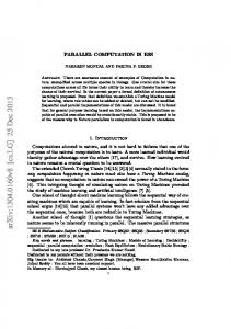
Fig. 1. Compressing X (I × J × K) to Y p (Lp × Mp × Np ) by multiplying T (every slab of) X from the I-mode with UT p , from the J-mode with Vp , and from the K-mode with WpT .
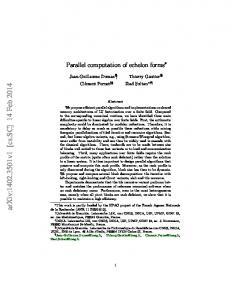
compressed tensors Y1 , . . . , YP is independently decomposed e p, B e p and C e p with a rank of F , into CP factors denoted by A for p = 1, . . . , P , using, for example, the ALS algorithm as described in Section II. Finally, the F factors are “joined” to compute A, B and C, the rank F decomposition of the big tensor X. This process is depicted in Figure 2. PARACOMP is particularly attractive due to its natural parallel structure and the fact that the big tensor data does not need to be repeatedly accessed for the decomposition. The initial compression stage, however, can be a bottleneck. On the bright side, (12) can be performed “in place”, requires only bounded intermediate memory, and it can exploit sparsity by summing only over the non-zero elements of X. On the other hand, complexity is O(LM N IJK) for a dense tensor, and O(LM N (NNZ)) for a sparse tensor. The main issue with (12), however, is that it features a terrible memory access pattern which can really bog down computations. An alternative computation schedule comprises three steps: T1 (l, j, k) =
compression matrices Up ∈ RI×Lp , Vp ∈ RJ×Mp and Wp ∈ RK×Np , the compressed tensor Yp ∈ RLp ×Mp ×Np computed as Yp (l, m, n) = I ∑ J ∑ K ∑
I ∑
U(l, i)X(i, j, k),
i=1
∀l ∈ {1, . . . , Lp } , j ∈ {1, . . . , J} , k ∈ {1, . . . , K} (13) J ∑ T2 (l, m, k) = V(m, j)T1 (l, j, k), j=1
Up (l, i)Vp (m, j)Wp (n, k)X(i, j, k)
(12)
i=1 j=1 k=1
for l ∈ {1, . . . , Lp }, m ∈ {1, . . . , Mp } and n ∈ {1, . . . , Np }. The compression operation in (12) can be thought of as multiplying (and compressing) the big tensor X by UTp along the first mode, VpT along the second mode, and WpT along the third mode. This corresponds to compressing each of the dimensions of X independently, i.e., reducing the dimension I to Lp , J to Mp and K to Np . The result is a smaller “cube” of dimensions Lp ×Mp ×Np . This process is depicted in Figure 1. This computation is repeated for p = 1, . . . , P , for some P and
The PARACOMP fork-join architecture. { }P The fork creates P randomly compressed reduced-size ‘replicas’ Y p , obtained by applying
Fig. 2.
p=1
(Up , Vp , Wp ) to X, as in Fig. 1. Each Y p is independently factored. ( ) ˜ p, B ˜ p, C ˜p , The join collects the estimated mode loading sub-matrices A anchors them all to a common permutation and scaling, and solves a linear least squares problem to estimate (A, B, C).
L1 , . . . , LP