Merlin: specification inference for explicit ... - Semantic Scholar

Merlin: Specification Inference for Explicit Information Flow Problems Benjamin Livshits, Aditya V. Nori, Sriram K. Rajamani

Anindya Banerjee ∗

Microsoft Research

IMDEA Software, Madrid, Spain

Abstract

analyzed with C AT.N ET, a state-of-the-art static analysis tool for .NET. We find a total of 167 new confirmed specifications, which result in a total of 322 additional vulnerabilities across the 10 benchmarks. More accurate specifications also reduce the false positive rate: in our experiments, M ERLIN-inferred specifications result in 13 false positives being removed; this constitutes a 15% reduction in the C AT.N ET false positive rate on these 10 programs. The final false positive rate for C AT.N ET after applying M ERLIN in our experiments drops to under 1%.

The last several years have seen a proliferation of static and runtime analysis tools for finding security violations that are caused by explicit information flow in programs. Much of this interest has been caused by the increase in the number of vulnerabilities such as cross-site scripting and SQL injection. In fact, these explicit information flow vulnerabilities commonly found in Web applications now outnumber vulnerabilities such as buffer overruns common in type-unsafe languages such as C and C++. Tools checking for these vulnerabilities require a specification to operate. In most cases the task of providing such a specification is delegated to the user. Moreover, the efficacy of these tools is only as good as the specification. Unfortunately, writing a comprehensive specification presents a major challenge: parts of the specification are easy to miss, leading to missed vulnerabilities; similarly, incorrect specifications may lead to false positives. This paper proposes M ERLIN, a new approach for automatically inferring explicit information flow specifications from program code. Such specifications greatly reduce manual labor, and enhance the quality of results, while using tools that check for security violations caused by explicit information flow. Beginning with a data propagation graph, which represents interprocedural flow of information in the program, M ERLIN aims to automatically infer an information flow specification. M ERLIN models information flow paths in the propagation graph using probabilistic constraints. A na¨ıve modeling requires an exponential number of constraints, one per path in the propagation graph. For scalability, we approximate these path constraints using constraints on chosen triples of nodes, resulting in a cubic number of constraints. We characterize this approximation as a probabilistic abstraction, using the theory of probabilistic refinement developed by McIver and Morgan. We solve the resulting system of probabilistic constraints using factor graphs, which are a well-known structure for performing probabilistic inference. We experimentally validate the M ERLIN approach by applying it to 10 large business-critical Web applications that have been

Categories and Subject Descriptors D.3.4 [Processors]: Compilers; D.4.6 [Operating Systems]: Security and Protection— Information flow controls; D.2.4 [Software/Program Verification]: Statistical methods General Terms Languages, Security, Verification Keywords Security analysis tools, Specification inference

1.

Introduction

Constraining information flow is fundamental to security: we do not want secret information to reach untrusted principals (confidentiality), and we do not want untrusted principals to corrupt trusted information (integrity). If we take confidentiality and integrity to the extreme, then principals from different levels of trust can never interact, and the resulting system becomes unusable. For instance, such a draconian system would never allow a trusted user to view untrusted content from the Internet. Thus, practical systems compromise on such extremes, and allow flow of sanitized information across trust boundaries. For instance, it is unacceptable to take a string from untrusted user input, and use it as part of a SQL query, since it leads to SQL injection attacks. However, it is acceptable to first pass the untrusted user input through a trusted sanitization function, and then use the sanitized input to construct a SQL query. Similarly, confidential data needs to be cleansed to avoid information leaks. Practical checking tools that have emerged in recent years [4, 21, 24] typically aim to ensure that all explicit flows of information across trust boundaries are sanitized. The fundamental program abstraction used in the sequel (as well as by existing tools) is what we term the propagation graph — a directed graph that models all interprocedural explicit information flow in a program.1 The nodes of a propagation graph are methods, and edges represent explicit information flow between methods. There is an edge from node m1 → m2 whenever there is a flow of information from method m1 to method m2 , through a method

Permission to make digital or hard copies of all or part of this work for personal or classroom use is granted without fee provided that copies are not made or distributed for profit or commercial advantage and that copies bear this notice and the full citation on the first page. To copy otherwise, to republish, to post on servers or to redistribute to lists, requires prior specific permission and/or a fee. PLDI’09, June 15–20, 2009, Dublin, Ireland. c 2009 ACM 978-1-60558-392-1/09/06. . . $5.00 Copyright !

1 We do not focus on implicit information flows [27] in this paper: discussions with C AT.N ET [21] developers reveal that detecting explicit information flow vulnerabilities is a more urgent concern. Existing commercial tools in this space exclusively focus on explicit information flow.

∗ Partially

supported at Kansas State University by NSF grants ITR0326577 and CNS-0627748 and by Microsoft Research, Redmond, by way of a sabbatical visit.

75

agation graph are secure can be modeled using one probabilistic constraint for each path in the propagation graph. A probabilistic constraint is a path constraint parameterized by the probability that the constraint is true. By solving these constraints, we can get assignments to values of these random variables, which yields an information flow specification. In other words, we use probabilistic reasoning and the intuition we have about the outcome of the constraints (i.e, the probability of each constraint being true) to calculate values for the inputs to the constraints. Since there can be an exponential number of paths, using one constraint per path does not scale. In order to scale, we approximate the constraints using a different set of constraints on chosen triples of nodes in the graph. We show that the constraints on triples are a probabilistic abstraction of the constraints on paths (see Section 5) according to the theory developed by McIver and Morgan [19, 20]. As a consequence, we can show that approximation using constraints on triples does not introduce false positives when compared with the constraints on paths. After studying large applications, we found that we need additional constraints to reduce false positives, such as constraints to minimize the number of inferred sanitizers, and constraints to avoid inferring wrappers as sources or sinks. Section 2 describes these observations and constraints in detail. We show how to model these observations as additional probabilistic constraints. Once we have modeled the problem as a set of probabilistic constraints, specification inference reduces to probabilistic inference. To perform probabilistic inference in a scalable manner, M ERLIN uses factor graphs, which have been used in a variety of applications [12, 35]. While we can use the above approach to infer specifications without any prior specification, we find that the quality of inference is significantly higher if we use the default specification that comes with the static analysis tool as the initial specification, using M ERLIN to “complete” this partial specification. Our empirical results in Section 6 demonstrate that our tool provides significant value in both situations. In our experiments, we use C AT.N ET [21], a state-of-the-art static analysis tool for finding Web application security flaws that works on .NET bytecode. The initial specification provided by C AT.N ET is modeled as extra probabilistic constraints on the random variables associated with nodes of the propagation graph. To show the efficacy of M ERLIN, we show empirical results for 10 large Web applications.

1. void ProcessRequest(HttpRequest request, 2. HttpResponse response) 3. { 4. string s1 = request.GetParameter("name"); 5. string s2 = request.GetHeader("encoding"); 6. 7. response.WriteLine("Parameter " + s1); 8. response.WriteLine("Header " + s2); 9. }

Figure 1. Simple cross-site scripting example parameter, or through a return value, or by way of an indirect update through a pointer. Following the widely accepted Perl taint terminology conventions [30] — more precisely defined in [14] — nodes of the propagation graph are classified as sources, sinks, and sanitizers; nodes not falling in the above categories are termed regular nodes. A source node returns tainted data whereas it is an error to pass tainted data to a sink node. Sanitizer nodes cleanse or untaint or endorse information to mediate across different levels of trust. Regular nodes do not taint data, and it is not an error to pass tainted data to regular nodes. If tainted data is passed to regular nodes, they merely propagate it to their successors without any mediation. A classification of nodes in a propagation graph into sources, sinks and sanitizers is called an information flow specification or, just specification for brevity. Given a propagation graph and a specification, one can easily run a reachability algorithm to check if all paths from sources to sinks pass through a sanitizer. In fact, this is precisely what many commercial analysis tools in everyday use do [4, 24]. User-provided specifications, however, lead to both false positives and false negatives in practice. False positives arise because a flow from source to sink classified as offending by the tool could have a sanitizer that the tool was unaware of. False negatives arise because of incomplete information about sources and sinks. This paper presents M ERLIN, a tool that automatically infers information flow specifications for programs. Our inference algorithm uses the intuition that most paths in a propagation graph are secure. That is, most paths in the propagation graph that start from a source and end in a sink pass through some sanitizer. Example 1 Consider a Web application code snippet written in C# shown in Figure 1. While method GetParameter, the method returning arguments of an HTTP request, is highly likely to be part of the default specification that comes with a static analysis tool and classified as a source, the method retrieving an HTTP header GetHeader may easily be missed. Because response.WriteLine sends information to the browser, there are two possibilities of cross-site scripting vulnerabilities on line 7 and line 8. The vulnerability in line 7 (namely, passing a tainted value returned by GetParameter into WriteLine without saniziting it first) will be reported, but the similar vulnerability on line 8 may be missed due to an incomplete specification. In fact, in both .NET and J2EE there exist a number of source methods that return various parts of an HTTP request. When we run M ERLIN on larger bodies of code, even within the HttpRequest class alone, M ERLIN correctly determines that getQueryString, getMethod, getEncoding, and others are sources missing from the default specification that already contains 111 elements. While this example is small, it is meant to convey the challenge involved in identifying appropriate APIs for an arbitrary application. !

Contributions. Our paper makes the following contributions: • M ERLIN is the first practical approach to inferring specifica-

tions for explicit information flow analysis tools, a problem made important in recent years by the proliferation of information flow vulnerabilities in Web applications.

• A salient feature of our method is that our approximation (us-

ing triples instead of paths) can be characterized formally — we make a connection between probabilistic constraints and probabilistic programs, and use the theory of probabilistic refinement developed by McIver and Morgan [19, 20] to show refinement relationships between sets of probabilistic constraints. As a result, our approximation does not introduce false positives.

• M ERLIN is able to successfully and efficiently infer information

flow specifications in large code bases. We provide a comprehensive evaluation of the efficacy and practicality of M ERLIN using 10 Web application benchmarks. We find a total of 167 new confirmed specifications, which result in a total of 322 vulnerabilities across the 10 benchmarks that were previously undetected. M ERLIN-inferred specifications also result in 13 false positives being removed.

Our approach. M ERLIN infers information flow specifications using probabilistic inference. By using a random variable for each node in the propagation graph to denote whether the node is a source, sink or sanitizer, the intuition that most paths in a prop-

76

INITIAL  SPECIFICATION

refine the specification

Specification Inference PROGRAM

STATIC  ANALYSIS

FINAL G

FACTOR GRAPH  CONSTRUCTION

F

PROBABILISTIC

SPECIFICATION

INFERENCE

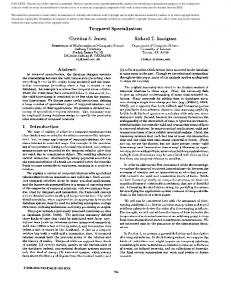
Figure 2. M ERLIN system architecture. Outline. The rest of the paper is organized as follows. Section 2 gives motivation for the specification inference techniques M ERLIN uses. Section 3 provides background on factor graphs. Section 4 describes our algorithm in detail. Section 5 proves that the system of triple constraints is a probabilistic abstraction over the system of path constraints. Section 6 describes our experimental evaluation. Finally, Sections 7 and 8 describe related work and conclude.

2.

public void TestMethod1() { string a = ReadData1(); string b = Prop1(a); string c = Cleanse(b); WriteData(c); }

ReadData1

ReadData2

Prop1

Prop2

public void TestMethod2() { string d = ReadData2(); string e = Prop2(d); string f = Cleanse(e); WriteData(f); }

Overview

Cleanse

WriteData

In addition to two top-level “driver” methods, TestMethod1 and TestMethod2, this code uses six methods: ReadData1, ReadData2, Prop1, Prop2, Cleanse, and WriteData. This program gives rise to the propagation graph shown on the right. An edge in the propagation graph represents explicit flow of data; i.g., the value returned by Prop1 is passed into Cleanse as an argument. The edge from Prop1 to Cleanse represents this flow. !

Figure 2 shows an architectural diagram of M ERLIN. M ERLIN starts with an initial, potentially incomplete specification of the application to produce a more complete specification. Returning to Example 1, suppose we start M ERLIN with an initial specification that classifies GetParameter as a source and WriteLine as a sink. Then, the specification output by M ERLIN would additionally contain GetHeader as a source. In addition to the initial specification, M ERLIN also consumes a propagation graph, a representation of the interprocedural data flow. Nodes of the propagation graph are methods in the program, and edges represent explicit flow of data.

2.1

Assumptions and Probabilistic Inference

The crux of our approach is probabilistic inference: we first use the propagation graph to generate a set of probabilistic constraints and then use probabilistic inference to solve them. M ERLIN uses factor graphs (see Section 3) to perform probabilistic inference efficiently. As shown in Figure 2, M ERLIN performs the following steps: 1) construct a factor graph based on the propagation graph; 2) perform probabilistic inference on the factor graph to derive the likely specification. M ERLIN relies on the assumption that most paths in the propagation graph are secure. That is, most paths that go from a source to a sink pass through a sanitizer. The assumption that errors are rare has been used before in other specification inference techniques [3, 10]. Further, we assume that the number of sanitizers is small, relative to the number of regular nodes. Indeed, developers typically define a small number of sanitization functions or use ones supplied in libraries, and call them extensively. For instance, the out-of-box specification that comes with C AT.N ET summarized in Figure 12 contains only 7 sanitizers. However, as we show later in this section, applying these assumptions along various paths individually can lead to inconsistencies, since the constraints inferred from different paths can be mutually contradictory. Thus, we need to represent and analyze each path within a constraint system that tolerates uncertainty and contradictions. Therefore, we parameterize each constraint with the probability of its satisfaction. These probabilistic constraints model the relative positions of sources, sinks, and sanitizers in the propagation graph. Our goal is to classify each node as a source, sink,

Definition 1. A propagation graph is a directed graph G = "NG , EG #, where nodes NG are methods and an edge (n1 → n2 ) ∈ Eg indicates that there is a flow of information from method n1 to method n2 through method arguments, or return values, or indirectly through pointers. The propagation graph is a representation of the interprocedural data flow produced by static analysis of the program. Due to the presence of virtual functions, and information flow through references, a pointer analysis is needed to produce a propagation graph. Since pointer analyses are imprecise, edges of a propagation graph approximate information flows. Improving the accuracy of propagation graph involves improving the precision of pointer analysis, and is beyond the scope of this paper. In our implementation, C AT.N ET uses an unsound pointer analysis, so there could be flows of data that our propagation graph does not represent. Even though propagation graphs can have cycles, M ERLIN performs a breadthfirst search and deletes the edges that close cycles, resulting in an acyclic propagation graph. Removing cycles greatly simplifies the subsequent phases of M ERLIN. As our empirical results show, even with such approximations in the propagation graph, M ERLIN is able to infer useful specifications. Example 2 We illustrate propagation graphs with an example.

77

A1

B1

B2

B3 B4

B5

B1: Triple safety. In order to abstract the constraint set A1 with a polynomial number of constraints, we add a safety constraint B1 for each triple of nodes as shown in Figure 3. The number of B1 constraints is O(N 3 ). In Section 5 we prove that the constraints B1 are a probabilistic abstraction of constraints A1 under suitable choices of parameters.

For every acyclic path m1 , m2 , . . . , mk−1 , mk , where m1 is a potential source and mk is a potential sink, the joint probability of classifying m1 as a source, mk as a sink and all of m2 , . . . , mk−1 as regular nodes is low. For every triple of nodes "m1 , m2 , m3 #, where m1 is a potential source, m3 is a potential sink, and m1 and m3 are connected by a path through m2 in the propagation graph, the joint probability that m1 is a source, m2 is not a sanitizer, and m3 is a sink is low. For every pair of nodes "m1 , m2 # such that both m1 and m2 lie on the same path from a potential source to a potential sink, the probability of both m1 and m2 being sanitizers is low. Each node m is classified as a sanitizer with probability s(m) (see Definition 3 for definition of s). For every pair of nodes "m1 , m2 # such that both m1 and m2 are potential sources, and there is a path from m1 to m2 the probability that m1 is a source and m2 is not a source is high. For every pair of nodes "m1 , m2 # such that both m1 and m2 are potential sinks, and there is a path from m1 to m2 the probability that m2 is a sink and m1 is not a sink is high.

2.4

In practice, the set of constraints B1 does not limit the solution space enough. We have found empirically that just using this set of constraints allows too many possibilities, several of which are incorrect classifications. By looking at results over several large benchmarks we have come up with four sets of auxiliary constraints B2, B3, B4, and B5, which greatly enhance the precision. B2: Pairwise Minimization. The set of constraints B1 allows the solver flexibility to consider multiple sanitizers along a path. In general, we want to minimize the number of sanitizers we infer. Thus, if there are several solutions to the set of constraints B1, we want to favor solutions that infer fewer sanitizers, while satisfying B1, with higher probability. For instance, consider the path ReadData1, Prop1, Cleanse, WriteData in Example 2. Suppose ReadData1 is a source and WriteData is a sink. B1 constrains the triple "ReadData1, Prop1, WriteData#

so that the probability of Prop1 not being a sanitizer is low; B1 also constrains the triple

Figure 3. Constraint formulation. Probabilities in italics are parameters of the constraints.

"ReadData1, Cleanse, WriteData#

such that the probability of Cleanse not being a sanitizer is low. One solution to these constraints is to infer that both Prop1 and Cleanse are sanitizers. In reality, programmers do not add multiple sanitizers on a path and we believe that only one of Prop1 or Cleanse is a sanitizer. Thus, we add a constraint B2 that for each pair of potential sanitizers it is unlikely that both are sanitizers, as shown in Figure 3. The number of B2 constraints is O(N 2 ).

sanitizer, or a regular node, so as to optimize satisfaction of these probabilistic constraints. 2.2

Potential Sources, Sinks and Sanitizers

The goal of specification inference is to classify nodes of the propagation graph into sources, sinks, sanitizers, and regular nodes. Since we are interested in string-related vulnerabilities, we first generate a set of potential sources, potential sanitizers, and potential sinks based on method signatures, as defined below:

Need for probabilistic constraints. Note that constraints B1 and B2 can be mutually contradictory, if they are modeled as non-probabilistic boolean constraints. For example, consider the propagation graph of Example 2. With each of the nodes ReadData1, WriteData, Prop1, Cleanse let us associate boolean variables r1 , w, p1 and c respectively. The interpretation is that r1 is true iff ReadData1 is source, w is true iff WriteData is a sink, p1 is true iff Prop1 is a sanitizer, and c is true iff Cleanse is a sanitizer. Then, constraint B1 for the triple "ReadData1, Prop1, WriteData# is given by the boolean formula r1 ∧ w =⇒ p1 , and the constraint B1 for the triple "ReadData1, Cleanse, WriteData# is given by the formula r1 ∧ w =⇒ c. Constraint B2 for the pair "Prop1, Cleanse# states that both Prop1 and Cleanse cannot be sanitizers, and is given by the formula ¬(p1 ∧ c). In addition, suppose we have additional information (say, from a partial specification given by the user) that ReadData1 is indeed a source, and WriteData is a sink. We can conjoin all the above constraints to get the boolean formula:

• Methods that produce strings as output are classified as poten-

tial sources.

• Methods that take a string as input, and produce a string as

output are classified as potential sanitizers.

• Methods that take a string as input, and do not produce a string

as output are classified as potential sinks.

Next, we perform probabilistic inference to infer a subset of potential sources, potential sanitizers, and potential sinks that form the inferred specification. 2.3

Auxiliary Constraints

Core Constraints

Figure 3 summarizes the constraints that M ERLIN uses for probabilistic inference. We describe each of the constraints below referring to Example 2 where appropriate. We also express the number of constraints of each type as a function of N , the number of nodes in the propagation graph.

(r1 ∧ w =⇒ p1 ) ∧ (r1 ∧ w =⇒ c) ∧ ¬(p1 ∧ c) ∧ r1 ∧ w

This formula is unsatisfiable and these constraints are mutually contradictory. Viewing them as probabilistic constraints gives us the flexibility to add such conflicting constraints; the probabilistic inference resolves such conflicts by favoring satisfaction of those constraints with higher probabilities attached to them.

A1: Path safety. We assume that most paths from a source to a sink pass through at least one sanitizer. For example, we believe that if ReadData1 is a source, and WriteData is a sink, at least one of Prop1 or Cleanse is a sanitizer. This is stated using the set of constraints A1 shown in Figure 3. While constraints A1 model our core beliefs accurately, they are inefficient if used directly: A1 requires one constraint per path, and the number of acyclic paths could be exponential in the number of propagation graph nodes.

B3: Sanitizer Prioritization. We wish to bias the selection of sanitizers to favor those nodes that have a lot of source-to-sink paths going through them. We formalize this below.

78

Definition 2. For each node m define weight W (m) to be the total number of paths from sources to sinks that pass through m.

where the sum is over all variables except xi . The marginal probability for each variable defines the solution that we are interested in computing. Intuitively, these marginals correspond to the likelihood of each boolean variable being equal to true or false. Factor graphs [35] fC1 fC2 are graphical models that are used for computing marginal probabilities efficiently. These graphs x1 x2 x3 take advantage of their structure in order to speed Figure 4. Factor graph for (3). up the marginal probability computation (known as probabilistic inference). There are a wide variety of techniques for performing probabilistic inference on a factor graph and the sum-product algorithm [35] is the most practical algorithm among these. Let the joint probability distribution p(x1 , . . . , xN ) be a product of factors as follows:

Suppose we know that ReadData1 is a source, ReadData2 is not a source, and WriteData is a sink. Then W (Prop1) = W (Cleanse) = 1, since there is only one source-to-sink path that goes through each of them. However, in this case, we believe that Prop1 is more likely to be a sanitizer than Cleanse since all paths going through Prop1 are source-to-sink paths and only some paths going through Cleanse are source-to-sink paths. Definition 3. For each node m define Wtotal (m) to be the total number of paths in the propagation graph that pass through the node m (this includes both source-to-sink paths, as well as other paths). Let us define s(m) for each node m as follows: s(m) =

W (m) Wtotal (m)

We add a constraint B3 that prioritizes each potential sanitizer n based on its s(n) value, as shown in Figure 3. The number of B3 constraints is O(N ).

p(x1 , . . . , xN ) =

• Variable nodes: one node for every variable xi . • Function nodes: one node for every function fs .

Example 3 As an example, consider the following formula (x1 ∨ x2 ) ∧ (x1 ∨ ¬x3 ) C1

where

···

p(x1 , . . . , xN )

0.9 if x1 ∨ ¬x3 = true (9) 0.1 otherwise If we use this interpretation of fC1 and fC2 , then we can interpret formula 5 as a probabilistic constraint.

(1)

fC1 (x1 , x2 ) × fC2 (x1 , x3 ) Z

(10)

(fC1 (x1 , x2 ) × fC2 (x1 , x3 ))

(11)

p(x1 , x2 , x3 ) =

xN

p(x1 , . . . , xN )

(6)

fC2 =

where

where xi ∈ {true, false} for i ∈ [1, . . . , N ]. Since there are an exponential number of terms in Equation 1, a na¨ıve algorithm for computing pi (xi ) will not work in practice. An abbreviated notation for Equation 1 is pi (xi ) =

if x1 ∨ x2 = true otherwise

1 if x1 ∨ ¬x3 = true (7) 0 otherwise The factor graph for this formula is shown in Fig. 4. There are three variable nodes for each variable xi , 1 ≤ i ≤ 3 and a function node fCj for each clause Cj , j ∈ {1, 2}. Equations 6 and 7 can also be defined probabilistically thus allowing for solutions that do not satisfy formula 4; but such solutions are usually set up such that they occur with low probability as shown below: 0.9 if x1 ∨ x2 = true fC1 = (8) 0.1 otherwise

In the previous section, we have described a set of probabilistic constraints that are generated from an input propagation graph. The conjunction of these constraints can be looked upon as a joint probability distribution over random variables that measure the odds of propagation graph nodes being sources, sanitizers, or sinks. Let p(x1 , . . . , xN ) be a joint probability distribution over boolean variables x1 , . . . , xN . We are interested in computing the marginal probabilities pi (xi ) defined as: xi−1 xi+1

1 0

(5)

fC2 =

Factor Graph Primer

···

f (x1 , x2 , x3 ) = fC1 (x1 , x2 ) ∧ fC2 (x1 , x3 ) fC1 =

Given a propagation graph with N nodes, we can generate the constraints B1 through B5 in O(N 3 ) time. Next, we present some background on factor graphs, an approach to efficiently solving probabilistic constraints.

x1

(4)

C2

Equation 4 can be rewritten as:

B5: Sink Wrapper Avoidance. Wrappers on sinks can be handled similarly, with the variation that in the case of sinks the data actually flows from the wrapper to the sink. We add a constraint B5 for each pair of potential sinks as shown in Figure 3. The number of B5 constraints is O(N 2 ).

pi (xi ) =

(3)

where xs is the set of variables involved in the factor fs . A factor graph is a bipartite graph that represents this factorization. A factor graph has two types of nodes:

B4: Source Wrapper Avoidance. Similar to avoiding inference of multiple sanitizers on a path, we also wish to avoid inferring multiple sources on a path. A prominent issue with inferring sources is the issue of having wrappers, i.e. functions that return the result produced by the source. For instance, if an application defines their own series of wrappers around system APIs, which is not uncommon, there is no need to flag those as sources because that will actually not affect the set of detected vulnerabilities. In such cases, we want M ERLIN to infer the actual source rather than the wrapper function around it. We add a constraint B4 for each pair of potential sources as shown in Figure 3. The number of B4 constraints is O(N 2 ).

3.

fs (xs ) s

Z= x1 ,x2 ,x3

is the normalization constant. The marginal probabilities are defined as pi (xi ) = p(!x), 1 ≤ i ≤ 3 (12)

(2)

∼{xi }

∼{xi }

79

ComputeWAndSValues(G:Propagation Graph, Xsrc , Xsan , Xsnk : Set of Nodes) Precondition: Inputs: Acyclic propagation graph G, sets of nodes Xsrc , Xsan , Xsnk representing potential sources, potential sanitizers and potential sinks respectively Returns: W (n) and s(n) for each potential sanitizer n in G

GenFactorGraph Inputs: (G = "V, E# : P ropagationGraph), parameters low1 , low2 , high1 , high2 , high3 , high4 ∈ [0..1] Returns: a factor graph F for the propagation graph G

1: G" = MakeAcyclic(G) 2: "Xsrc , Xsan , Xsnk # = ComputePotentialSrcSanSnk(G) 3: "Triples, Pairssrc , Pairssan , Pairssnk #=

1: for each potential source n ∈ Xsrc do 2: F (n) := initial probability of n being a source node 3: Ftotal (n) := 1 4: end for 5: for each potential sanitizer n ∈ Xsan in topological order do 6: F (n) := 0 7: Ftotal (n) := 0 8: for each m ∈ V such that (m, n) ∈ E do 9: F (n) := F (n) + F (m) 10: Ftotal (n) := Ftotal (n) + Ftotal (m) 11: end for 12: end for 13: for each potential sink n ∈ Xsnk do 14: B(n) := initial probability of n being a sink node 15: Btotal (n) := 1 16: end for 17: for each potential sanitizer n ∈ Xsan in reverse topological order do 18: B(n) := 0 19: Btotal (n) := 0 20: for each m ∈ V such that (n, m) ∈ E do 21: B(n) := B(n) + B(m) 22: Btotal (n) := Btotal (n) + Btotal (m) 23: end for 24: end for 25: for each potential sanitizer n ∈ Xsan do 26: W (n) := F (n) ∗ B(n) W (n) 27: s(n) := F total (n)∗Btotal (n) 28: end for 29: return s

"

ComputePairsAndTriples(G , Xsrc , Xsan , Xsnk )

4: s = ComputeWAndSValues(G" ) 5: for each triple "a, b, c# ∈ Triples do 6: Create a factor fB1 (xa , xb , xc ) in the factor graph 7: Let fB1 (xa , xb , xc ) = xa ∧ ¬xb ∧ xc 8: Let probability Pr(fB1 (xa , xb , xc ) = true) = low1 9: end for 10: for each pair "b1 , b2 # ∈ Pairssan do 11: Create a factor fB2 (xb1 , xb2 ) in the factor graph 12: Let fB2 (xb1 , xb2 ) = xb1 ∧ xb2 13: Let probability Pr(fB2 (xb1 , xb2 ) = true) = low2 14: end for 15: for each n ∈ Xsan do 16: Create a factor fB3 (xn ) in the factor graph 17: Let fB3 (xn ) = xn 18: Let Pr(fB3 (xn ) = true) = s(n) 19: end for 20: for each pair "xa1 , xa2 # ∈ Pairssrc do 21: Create a factor fB4 (xa1 , xa2 ) in the factor graph 22: Let fB4 (xa1 , xa2 ) = xa1 ∧ ¬xa2 23: Let probability Pr(fB4 (xa1 , xa2 ) = true) = high3 24: end for 25: for each pair "xc1 , xc2 # ∈ Pairssnk do 26: Create a factor fB5 (xc1 , xc2 ) in the factor graph 27: Let fB5 (xc1 , xc2 ) = ¬xc1 ∧ xc2 28: Let probability Pr(fB5 (xc1 , xc2 ) = true) = high4 29: end for

Figure 6. Computing W (n) and s(n).

Figure 5. Generating a factor graph from a propagation graph.

These sets can be computed in O(N 3 ) time, where N is the number of nodes in the propagation graph. Next in line 4, the function ComputeWAndSValues is invoked to compute W (n) and s(n) for every potential sanitizer n. The function ComputeWAndSValues is described in Figure 6. In lines 5–9, the algorithm creates a factor node for the constraints B1. In lines 10–14, the algorithm iterates through all pairs "b1 , b2 # of potential sanitizers (that is, actual sanitizers as well as regular nodes) such that there is a path in the propagation graph from b1 to b2 and adds factors for constraints B2. In lines 15–19, the algorithm iterates through all potential sanitizers and adds factors for constraints B3. In lines 20–24, the algorithm iterates through all pairs "a1 , a2 # of potential sources such that there is a path in the propagation graph from a1 to a2 and adds factors for constraints B4. Similarly, in lines 25–29, the algorithm iterates through all pairs "c1 , c2 # of potential sinks such that there is a path from c1 to c2 and adds factors for constraints B5.

Here, pi (xi = true) denotes the fraction of solutions where the variable xi has value true. These marginal probabilities can be used to compute a solution to the SAT instance in Equation 4 as follows: (1) choose a variable xi with the highest marginal probability pi (xi ) and set xi = true, if pi (xi ) is greater than a threshold value, otherwise, set xi = f alse. (2) recompute the marginal probabilities and repeat Step (1) until all variables have been assigned (this is a satisfying assignment with high probability). Iterative message passing algorithms [12, 35] on factor graphs perform Steps (1) and (2) as well as compute marginal probabilities efficiently. !

4.

Constructing the Factor Graph

Given a propagation graph G, we describe how to build a factor graph F to represent the constraints B1 through B5 associated with G. Figure 5 shows the algorithm GenFactorGraph that we use to generate the factor graph from the propagation graph. The construction of the factor graph proceeds as follows. First, in line 1, the procedure MakeAcyclic converts the input propagation graph into a DAG G$ , by doing a breadth first search, and deleting edges that close cycles. Next, in line 2, the procedure ComputePotentialSrcSanSnk computes the sets of potential sources, potential sanitizers, and potential sinks, and stores the results in Xsrc , Xsan , and Xsnk , respectively. On line 3, procedure ComputePairsAndTriples computes four sets defined in Figure 7. These sets can be computed by first doing a topological sort of G$ (the acyclic graph), making one pass over the graph in topological order, and recording for each potential sanitizer the set of potential sources and potential sinks that can be reached from that node. Potential sources, sanitizers, and sinks are determined by analyzing type signatures of each method, as described in Section 2.2.

4.1

Computing s() and W ()

Recall values s() and W () defined in Section 2.4. Figure 6 describes ComputeWAndSValues, which computes s(n) for each potential sanitizer node, given input probabilities for each potential source and each potential sink. The value s(n) for each potential sanitizer n is the ratio of the sum of weighted source-sink paths that go through n and the total number of paths that go through n. The algorithm computes W (n) and s(n) by computing four numbers F (n), Ftotal (n), B(n), and Btotal (n). F (n) denotes the total number of sources that can reach n, and Ftotal (n) denotes the total number of paths that can reach n. B(n) denotes the total number of sinks that can be reached from

80

S ET

D EFINITION

Triples p∈paths(G" )

Pairssrc p∈paths(G" )

Pairssan p∈paths(G" )

Pairssnk p∈paths(G" )

{"xsrc , xsan , xsnk # | xsrc ∈ Xsrc , xsan ∈ Xsan , xsnk ∈ Xsnk , xsrc is connected to xsnk via xsan in p} {"xsrc , x$src #

| xsrc ∈ Xsrc , x$src ∈ Xsrc , xsrc is connected to x$src in p}

{"xsan , x$san #

| xsan ∈ Xsan , x$san ∈ Xsan , xsan is connected to x$san in p}

{"xsnk , x$snk #

| xsnk ∈ Xsnk , x$snk ∈ Xsnk , xsnk is connected to x$snk in p}

Figure 7. Set definitions for algorithm in Figure 5. Path(G = "V, E#) Returns: Mapping m from V to the set {0, 1}

Triple(G = "V, E#) Returns: Mapping m from V to the set {0, 1}

1: for all paths p = s, . . . , n from potential sources to sinks in G do 2: assume( m(p) '∈ 10∗ 1) ⊕cp assume(m(p) ∈ 10∗ 1) 3: end for

1: for all triples t = "s, w, n# such that s is a potential source, n is a potential sink and w lies on some path from s to n in G do

2: assume( m("s, w, n#) '= 101) ⊕ct assume( m("s, w, n#) = 101) 3: end for

Post expectation: [∀ paths p in G, m(p) '∈ 10∗ 1].

Post expectation: [∀ paths p in G, m(p) '∈ 10∗ 1].

Figure 9. Algorithm Path

Figure 10. Algorithm Triple

n. Finally, Btotal (n) denotes the total number of paths that can be reached from n. For each potential source n, we set F (n) to an initial value in line 2 (in our implementation, we picked an initial value of 0.5), and we set Ftotal (n) to 1 in line 3. For each potential sink, we set B(n) to some initial value in line 14 (in our implementation, we picked this initial value to be 0.5), and we set Btotal (n) to 1 in line 15. Since the graph G$ is a DAG, F (n) and Ftotal (n) can be computed by traversing potential sanitizers in topological sorted order, and B(n) and Btotal (n) can be computed by traversing potential sanitizers in reverse topological order. The computation of F (n) and Ftotal (n) in forward topological order is done in lines 5–12 and the computation of B(n) and Btotal (n) in reverse topological order is done in lines 17–24. Once F (n) and B(n) are computed, W (n) is set to F (n) × B(n) and s(n) is set to

B1 in Section 2. We use the theory of probabilistic abstraction and refinement developed by McIver and Morgan [19, 20] to derive appropriate bounds on probabilities associated with constraints A1 and B1 so that B1 is a probabilistic abstraction of the specification A1 (or, equivalently, A1 is a probabilistic refinement of B1). We first introduce some terminology and basic concepts from [20]. Probabilistic refinement primer. Non-probabilistic programs can be reasoned with assertions in the style of Floyd and Hoare [7]. The following formula in Hoare logic: {Pre} Prog {Post}

is valid if for every state σ satisfying the assertion Pre, if the program Prog is started at σ, then the resulting state σ $ satisfies the assertion Post. We assume Prog always terminates, and thus we do not distinguish between partial and total correctness. McIver and Morgan extend such reasoning to probabilistic programs [19, 20]. In order to reason about probabilistic programs, they generalize assertions to expectations. An expectation is a function that maps each state to a positive real number. If Prog is a probabilistic program, and Pre E and Post E are expectations, then the probabilistic Hoare-triple

W (n) W (n) = Ftotal (n) × Btotal (n) Wtotal (n)

as shown in line 26.

Parameter tuning. The parameters low1 , low2 , high1 , high2 , high3 , and high4 all need to be instantiated with any values between 0.0 and 1.0. In Section 5 we show how to compute parameter values for low1 associated with the constraints B1 from the parameter values for the constraints A1. We have experimented with varying the values of high1 , high2 , high3 and high4 from 0.8 to 0.95, and the low1 , low2 , values from 0.05 to 0.2 in increments as small as .01. Fortunately, our inference is quite robust: these parameter variations do not significantly affect the quality of results produced by the inference in the applications we have tried. Example 4 Figure 8 shows the factor graph obtained by applying algorithm FactorGraph to the propagation graph in Figure 2. The marginal probabilities for all variable nodes are computed by probabilistic inference on the factor graph and these are used to classify sources, sanitizers, and sinks in the propagation graph. !

5.

{Pre E } Prog {Post E }

is interpreted to mean the following: If the program Prog is started with an initial expectation Pre E , then it results in the expectation Post E after execution. Assertions are ordered by implication ordering. Expectations are ordered by the partial order ". Given two expectations AE and BE , we say that AE " BE holds if for all states σ, we have that AE (σ) ≤ BE (σ). Given an assertion A the expectation [A] is defined to map every state σ to 1 if σ satisfies A and to 0 otherwise. Suppose AE " BE . Consider a sampler that samples states using the expectations as a probability measure. Then, for any threshold t and state σ, if AE (σ) > t, then it is the case that BE (σ) > t. In other words, for any sampler with any threshold t, sampling over AE results in a subset of states than those obtained by sampling over BE . Traditional axiomatic proofs are done using weakest preconditions. The weakest precondition operator is denoted by WP. By

Relationship between Triples and Paths

In this section, we give a formal relationship between the exponential number of constraints A1 and the cubic number of constraints

81

fB3(xProp1)

fB2(xProp1,xCleanse)

xReadData1

fB1(xReadData1,xProp1, xWriteData)

xReadData2

fB3(xProp2)

xProp1

fB1(xReadData1,xProp1, xWriteData)

fB2(xProp2,xCleanse)

xProp2

xCleanse

fB1(xReadData2,xProp2, xWriteData)

fB3(xCleanse)

xWriteData

fB1(xReadData1,xProp1, xWriteData)

Figure 8. Factor graph for the propagation graph in Example 2. definition, for any program Prog and assertion A, we have that WP(Prog, A) to be the weakest assertion B (weakest is defined with respect to the implication ordering between assertions) such that the Hoare triple {B}Prog{A} holds. McIver and Morgan extend weakest preconditions to expectations, and define for an expectation AE , and a probabilistic program Prog, WP(Prog, AE ) is the weakest expectation BE (weakest is defined with respect to the ordering " between expectations) such that the probabilistic Hoare triple {BE }Prog{AE } holds. Given two probabilistic programs Spec and Impl with respect to a post expectation Post E , we say that Impl refines Spec if WP(Spec, Post E ) " WP(Impl, Post E ).

choose parameter values ct for each triple t in the program Triple such that Path refines Triple. Theorem. Consider any directed acyclic graph G = "V, E# and probabilistic programs Path (Figure 9) and Triple (Figure 10) with stated post expectations. Let the program Path have a parameter cp for each path p. For any such valuations to the cp ’s there exist parameter values for the Triple program, namely a parameter ct for each triple t such that the program Path refines the program Triple with respect to the post expectation Post E = [∀ paths p in G, m(p) +∈ 10∗ 1]. Proof: Consider any triple t = "s, w, n#. Choose the parameter ct for the triple t to be equal to the product of the parameters cp of all paths p in G that start at s, end at n and go through w. That is,

Refinement between constraint systems. We now model constraints A1 and B1 from Section 2 as probabilistic programs with an appropriate post expectation, and derive relationships between the parameters of A1 and B1 such that A1 refines B1. Consider any directed acyclic graph G = "V, E#, where E ⊆ V × V . In this simple setting, nodes with in-degree 0 are potential sources, nodes with out-degree 0 are potential sinks, and other nodes (internal nodes with both in-degree and out-degree greater than 0) are potential sanitizers. We want to classify every node in V with a boolean value 0 or 1. That is, we want a mapping m : V → {0, 1}, with the interpretation that for a potential source s ∈ V , m(s) = 1 means that s is classified as a source, and that for a potential sink n ∈ V , m(n) = 1 means that n is classified as a sink, and that for a potential sanitizer w ∈ V , m(w) = 1 means that w is classified as a sanitizer. We extend the mapping m to operate on paths (triples) over G by applying m to every vertex along the path (triple). We want mappings m that satisfy the constraint that for any path p = s, w1 , w2 , . . . , wm , n that starts at a potential source s and ends in a potential sink, the string m(p) +∈ 10∗ 1, where 10∗ 1 is the language of strings that begin and end with 1 and have a sequence of 0’s of arbitrary length in between. The constraint set A1 from Section 2 is equivalent in this setting to the probabilistic program Path given in Figure 9, and the constraint set B1 from Section 2 is equivalent in this setting to the probabilistic program Triple given in Figure 10. The statement assume(e) is a no-op if e holds and silently stops execution if e does not hold. The probabilistic statement S1 ⊕q S2 executes statement S1 with probability q and statement S2 with probability 1 − q. Note that both programs Path and Triple have the same post expectation [∀ paths p in G, m(p) +∈ 10∗ 1]. Further, note that both programs are parameterized. The Path program has a parameter cp associated with each path p in G, and the Triple program has a parameter ct associated with each triple t in G. The following theorem states that the probabilistic program Path refines program Triple under appropriate choices of probabilities as parameters. Furthermore, given a program Path with arbitrary values for the parameters cp for each path p, it is possible to

ct =

cp

(13)

p

such that t is a subsequence of p. To show that Path refines Triple with respect to the post expectation Post E stated in the theorem, we need to show that WP(Triple, Post E ) " WP(Path, Post E ). That is, for each state σ, we need to show that WP(Triple, Post E )(σ) ≤ WP(Path, Post E )(σ). Note that WP(assume(e), [A]) = [e ∧ A], and WP(S1 ⊕q S2 , [A]) = q × WP(S1 , [A]) + (1 − q) × WP(S2 , [A]) [20]. Using these two rules, we can compute WP(Triple, Post E ) and WP(Path, Post E ) as an expression tree which is a sum of product of expressions, where each product corresponds to a combination of probabilistic choices made in the program. First, consider any state σ that does not satisfy Post E . For this state, WP(Triple, Post E )(σ) = WP(Path, Post E )(σ) = 0, and the theorem follows trivially. Next, consider a state ω that satisfies Post E . In this case, WP(Path, Post E )(ω) is the product of probabilities cp for each path p in G. Also, in this case WP(Triple, Post E )(ω) is the product of two quantities X(ω) and Y (ω), where X(ω) is equal to the product of probabilities ct for each triple t = "s, w, n# such that m("s, w, n#) += 101, and Y (ω) is equal to the product of probabilities (1 − ct" ) for each triple t$ = "s$ , w$ , n$ # such that m("s$ , w$ , n$ #) = 101. Since ct ’s have been carefully chosen according to Equation 13 and Y (ω) ∈ [0, 1], it follows that X(ω) is less than or equal to the product of the probabilities cp for each path p. Therefore, it is indeed the case that for each state ω, WP(Triple, Post E )(ω) ≤ WP(Path, Post E )(ω). Any solver for a probabilistic constraint system C with post expectation Post E chooses states σ such that WP(C, Post E )(σ) is greater than some threshold t. Since we have proved that Path refines Triple, we know that every solution state for the Triple system, is also a solution state for the Path system. Thus, the set of states that are chosen by solver for the Triple system is contained in

82

Benchmark

DLLs

DLL size (kilobytes)

LOC

3 3 3 15 3 7 11 4 5 14

65 543 62 118 290 369 565 421 3,345 2,447

10,812 6,783 14,529 11,941 15,803 25,602 5,595 78,914 1,810,585 66,385

Alias Management Tool Chat Application Bicycle Club App Software Catalog Sporting Field Management Tool Commitment Management Tool New Hire Tool Expense Report Approval Tool Relationship Management Customer Support Portal

6.1

Figure 11 summarizes information about our benchmarks. As we discovered, not all code contained within the application source tree is actually deployed to the Web server. Most of the time, the number and size of deployed DLLs primarily consisting of .NET bytecode is a good measure of the application size, as shown in columns 2–3. Note that in a several cases, libraries supplied in the form of DLLs without the source code constitute the biggest part of an application. Finally, to provide another measure of the application size, column 4 shows the traditional line-of-code metric for all the code within the application. To put our results on specification discovery in perspective, Figure 12 provides information about the out-of-the box specification for C AT.N ET, the static analysis tool that we used for our experiments [21]. The second column shows the number of specifications for each specification type. The last column shows the number of revisions each portion of the specification has gone through, as extracted from the code revision repository. We have manually examined the revisions to only count substantial ones (i.e. just adding comments or changing whitespace was disregarded). It is clear from the table that even arriving at the default specification for C AT.N ET, as incomplete as it is, took a pretty significant number of source revisions. We found that most commonly revised specification correspond to most commonly found vulnerabilities. In particular, specifications for SQL injection and cross-site scripting attacks have been revised by far the most. Moreover, after all these revisions, the ultimate initial specification is also fairly large, consisting of a total of 111 methods. To provide a metric for the scale of the benchmarks relevant for C AT.N ET and M ERLIN analyses, Figure 13 provides statistics on the sizes of the propagation graph G computed by M ERLIN, and the factor graph F constructed in the process of constraint generation. We sort our benchmarks by the number of nodes in G. With propagation graphs containing thousands of nodes, it is not surprising that we had to develop a polynomial approximation in order for M ERLIN to scale, as Section 5 describes.

Figure 11. Benchmark application sizes. Type

Count

Revisions

Sources Sinks Sanitizers

27 77 7

16 8 2

Figure 12. Statistics for the out-of-the box specification that comes with C AT.N ET. the set of states that are chosen by the solver for the Path system. This has the desirable property that the Triple system will not introduce more false positives than the Path system. Note that the Path system itself can result in false positives, since it requires at least one sanitizer on each source-sink path, and does not require minimization of sanitizers. In order to remove false positives due to redundant sanitizers, we add the constraints B2 and B3 to the Triple system. Further, the path system does not distinguish wrappers of sources or sinks, so we add additional constraints B4 and B5 to avoid classifying these wrappers as sources or sinks. Using all these extra constraints, we find that the Triple system performs very well on several large benchmarks and infers specifications with very few false positives. We describe these results in the next section.

6.

6.2

Experimental Evaluation

G Alias Management Tool Chat Application Bicycle Club App Software Catalog Sporting Field Management Tool Commitment Management Tool New Hire Tool Expense Report Approval Tool Relationship Management Customer Support Portal

F

Nodes

Edges

Vars

Nodes

59 156 176 190 268 356 502 811 3,639 3,881

1,209 187 246 455 320 563 1,101 1,753 22,188 11,196

3 25 70 73 50 107 116 252 874 942

3 33 317 484 50 1,781 1,917 2,592 391,221 181,943

Merlin Findings

Figure 14 provides information about the specifications discovered by M ERLIN. Columns 2–16 provide information about how many correct and false positive items in each specification category has been found. Note that in addition to “good” and “bad” specifications, as indicated by #and !, we also have a “maybe” column denoted by ?. This is because often what constitutes a good specification is open to interpretation. Even in consultations with C AT.N ET developers we found many cases where the classification of a particular piece of the specification is not clear-cut. The column labeled Rate gives the false positive rate for M ERLIN: the percentage of “bad” specifications that were inferred. Overall, M ERLIN infers 381 specifications, out of which 167 are confirmed and 127 more are potential specifications. The M ERLIN false positive rate, looking at the discovered specifications is 22%, computed as (7+31+49)/381. This is decidedly better than the average state of the art false positive rate of over 90% [5]. The area in which M ERLIN does the worst is identifying sanitizers (with a 38% false positive rate). This is because despite the extra constraints described in Section 2.4, M ERLIN still flags some polymorphic functions as sanitizers. An example of this is the method NameValueCollection.get Item in the standard class library. Depending on what is stored in the collection, either the return result will be tainted or not. However, this function clearly does not untaint its argument and so is not a good sanitizer. Figure 15 summarizes information about the security vulnerabilities we find based on both the initial and the post-M ERLIN specifications. For the purpose of finding vulnerabilities, the post-

C AT.N ET, a publicly available state-of-the-art static analysis tool for Web application is the platform for our experiments [21]. M ER LIN is implemented as an add-on on top of C AT.N ET , using I N FER .NET, a library [22] that provides an interface to probabilistic inference algorithms. This section presents the results of evaluating M ERLIN on 10 large .NET Web applications. All these benchmarks are security-critical enterprise line-of-business applications currently in production written in C# on top of ASP.NET. They are also subject of periodic security audits.

Benchmark

Experimental Setup

Figure 13. Size statistics for the propagation graph G and factor graph F used by M ERLIN.

83

Benchmark Alias Management Tool Chat Application Bicycle Club App Software Catalog Sporting Field Management Tool Commitment Management Tool New Hire Tool Expense Report Approval Tool Relationship Management Customer Support Portal Total

S OURCES ? !

All

!

0 1 11 1 0 20 3 8 44 26

0 1 11 1 0 19 3 8 3 21

0 0 0 0 0 0 0 0 36 4

114

67

40

S ANITIZERS ? !

Rate

All

!

0 0 0 0 0 1 0 0 5 1

N/A 0% 0% 0% N/A 5% 0% 0% 11% 3%

0 0 3 8 0 9 1 20 1 39

0 0 2 3 0 1 1 2 0 16

0 0 0 0 0 2 0 13 0 10

7

6%

81

25

25

Rate

All

!

S INKS ?

!

Rate

0 0 1 5 0 6 0 5 1 13

N/A N/A 33% 62% N/A 66% 0% 25% 100% 33%

0 2 7 6 1 11 17 20 4 118

0 2 4 3 0 8 14 14 0 30

0 0 0 2 1 1 0 0 3 55

0 0 3 1 0 2 3 6 1 33

N/A 0% 42% 16% 0% 18% 17% 30% 25% 27%

31

38%

186

75

62

49

26%

Figure 14. New specifications discovered with M ERLIN. B EFORE

A FTER

Benchmark

All ! ? !

Alias Management Tool Chat Application Bicycle Club App Software Catalog Sporting Field Management Commitment Management Tool New Hire Tool Expense Report Approval Tool Relationship Management Customer Support Portal

2 2 0 0 0 0 14 8 0 0 1 1 4 4 0 0 9 6 59 19

Total

89 40 6 43 342 322 17 3 13

All

!

?

!

-

0 0 2 2 0 0 0 1 1 0 0 0 4 3 1 0 6 8 8 0 0 0 0 0 0 0 0 22 16 3 0 0 3 3 0 0 0 2 2 0 3 0 10 10 0 3 37 290 277 13

0 0 0 0 0 3 0 0 0 0

0 0 0 6 0 0 1 0 3 3

Figure 15. Vulnerabilities before and after M ERLIN. M ERLIN specifications we used are the “good” specifications denoted by the #columns in Figure 14. Columns 2–10 in Figure 15 show the number of vulnerabilities based on the original specification and the number of newly found vulnerabilities. Just like with specifications, we break down vulnerabilities into “good”, “maybe”, and “bad” categories denoted by #, ?, and !. The very last column reports 13 former false positives eliminated with the M ERLIN specification because of newly discovered sanitizers. As with many other static analysis tools, false positives is one of the primary complaints about C AT.N ET in practice. As can be seen from Figure 15 (the column marked with “−”), M ERLIN helps reduce the false positive rate from 48% to 33% (the latter computed as (43-13)/89). Furthermore, if we take into account all the 322 new (and confirmed) vulnerabilities into account, the false positive rate drops to 1% (computed as 3/342). Example 5 Function CreateQueryLink in Figure 16 is taken from the Software Catalog benchmark2 . The return result of this function is passed into a known cross-site redirection sink not shown here for brevity. • The paths that go through request.Url.AbsolutePath and

request.QueryString on lines 6 and 15 are correctly identified as new, not previously flagged vulnerabilities. • C AT.N ET flags the path that passes through function QueryStringParser.Parse on line 18 as a vulnerability. However, with M ERLIN, AntiXss.UrlEncode is correctly determined to be a sanitizer, eliminating this false positive. With M ERLIN, we eliminate all 6 false positives in this benchmark. 2 C AT.N ET addresses explicit information flow only and does not flag the fact that there is a control dependency on line 13 because tainted value request.QueryString is used within a conditional.

1 2 3 4 5 6 7 8 9 10 11 12 13 14 15 16 17 18 19 20 21 22 23 24 25 26 27 28 29

public static string CreateQueryLink( HttpRequest request, string key, string value, List keysToOmit, bool ignoreKey) { StringBuilder builder = new StringBuilder( request.Url.AbsolutePath); if (keysToOmit == null) { keysToOmit = new List(); } builder.Append("?"); for (int i = 0; i < request.QueryString.Count; i++) { if ((request.QueryString.GetKey(i) != key) && !keysToOmit.Contains(request.QueryString.GetKey(i))) { builder.Append(request.QueryString.GetKey(i)); builder.Append("="); builder.Append(AntiXss.UrlEncode( QueryStringParser.Parse( request.QueryString.GetKey(i)))); builder.Append("&"); } } if (!ignoreKey) { builder.Append(key); builder.Append("="); builder.Append(AntiXss.UrlEncode(value)); } return builder.ToString().TrimEnd(new char[] { ’&’ }); }

Figure 16. Function CreateQueryLink for Example 5. This short function illustrates many tricky issues with explicit information flow analyses as well as the danger of unrestricted manipulation of tainted data as strings. ! Note that while we start with the C AT.N ET specification characterized in Figure 12, M ERLIN can even infer specification entirely without an initial specification purely based on the structure of the propagation graph. Example 6 Consider a short program fragment written in C# consisting of two event handlers shown in Figure 17. When run 1 2 3 4 5 6 7 8 9 10 11

protected void TextChanged(object sender, EventArgs e) { string str = Request.QueryString["name"]; string str2 = HttpUtility.HtmlEncode(str); Response.Write(str2); } protected void ButtonClicked(object sender, EventArgs e) { string str = Request.UrlReferrer.AbsolutePath; string str2 = HttpUtility.UrlEncode(str); Response.Redirect(str2); }

Figure 17. Program for Example 6.

84

combining static and dynamic analysis for PHP programs. Several projects that came after WebSSARI improve on the quality of static analysis for PHP [9, 33]. The Griffin project proposes scalable and precise static and runtime analysis techniques for finding security vulnerabilities in large Java applications [15, 18]. Several other runtime systems for taint tracking have been proposed as well, including Haldar et al. [6] and Chandra et al. [1] for Java, Pietraszek et al. [25], and Nguyen-Tuong et al.for PHP [23]. Several commercial tools have been built to detect information flow vulnerabilities in programs [4, 24]. All these tools without exception require a specification of information flow. Our work infers such specifications.

Sources (1): string System.Web.HttpUtility+UrlDecoder.Getstring() Sanitizers (8): string System.Web.HttpUtility.HtmlEncode(string) string System.Web.HttpUtility.UrlEncodeSpaces(string) string System.Web.HttpServerUtility.UrlDecode(string) string System.Web.HttpUtility.UrlEncode(string, Encoding) string System.Web.HttpUtility.UrlEncode(string) string System.Web.HttpServerUtility.UrlEncode(string) string System.Web.HttpUtility.UrlDecodestringFrom... string System.Web.HttpUtility.UrlDecode(string, Encoding) Sinks (4): void System.Web.HttpResponse.WriteFile(string) void System.Web.HttpRequest.set_QuerystringText(string) void System.IO.TextWriter.Write(string) void System.Web.HttpResponse.Redirect(string)

7.2

A number of projects have addressed inferring specifications outside the context of security. For a general overview of specification mining techniques, the reader is referred to Perracotta [34], DynaMine [16], and Weimer et al. [31]. In particular, Engler et al. [3] infer specifications from code by seeking rules that involve action pairs: malloc paired with free, lock paired with unlock, etc. Li and Zhou [13] and Livshits and Zimmerman [16] look at more general patterns involving action pairs by combining data mining techniques as well as sophisticated pointer analyses. Whaley et al. [32] considers inference of interface specifications for Java method calls using static analysis. Jagannathan et al. [26] use data mining techniques for inference of method preconditions in complex software systems. The preconditions might incorporate data-flow as well as control-flow properties. Kremenek et al. [10] use probabilistic inference to classify functions that allocate and deallocate resources in programs. While similar in spirit to our work, inference of information flow specifications appears to be a more complex problem than inference of allocation and deallocation routines in C code in part because there are more classes classifications — sources, sinks, and sanitizers at play. Furthermore, the wrapper avoidance and sanitizer minimization constraints do not have direct analogs in the allocatordeallocator inference. Unlike Kremenek et al. [10] we use the theory of probabilistic refinement to formally characterize the triple approximation we have implemented for the purposes of scaling.

Figure 18. Specification inferred for Example 6.

Benchmark

C AT.N ET P

Alias Management Tool Chat Application Bicycle Club App Software Catalog Sporting Field Management Tool Commitment Management Tool New Hire Tool Expense Report Approval Tool Relationship Management Customer Support Portal

2.64 4.61 2.81 3.94 5.97 6.41 7.84 7.27 55.38 89.75

M ERLIN G F 4.59 .81 .53 1.02 2.22 18.84 2.98 3.59 87.63 29.75

2.63 2.67 2.72 2.73 2.69 2.91 3.44 3.05 66.45 31.55

Total time 9.86 8.09 6.06 7.69 10.88 28.16 14.27 13.91 209.45 151.05

Figure 19. Static analysis and specification inference running time, in seconds. with no intial specification at all, M ERLIN is able to infer a small, but absolutely correct specification consisting of 13 elements, as shown in Figure 18. Starting with even a small specification such as the one above, M ERLIN is able to succesfully infer increasingly larger specifications that fill many gaps in the original C AT.N ET specification. ! 6.3

8.

Running Times

Finally, Figure 19 provides information about running time of the various M ERLIN components, measured in seconds. Columns 2–4 show the C AT.N ET running time, the time to build the propagation graph, and the inference time. The experiments were conducted on a 3 GHz Pentium Dual Core Windows XP SP2 machine equipped with 4 GB of memory. Overall, in part due to the approximation described in Section 5, our analysis scales quite well, with none of the benchmarks taking over four minutes to analyze. Given that C AT.N ET is generally run once a day or less frequently, these running times are more than acceptable.

7.

Conclusions

The growing importance of explicit information flow is evidenced by the abundance of analysis tools for information flow tracking and violation detection at the level of the language, runtime, operating system, and hardware [1, 2, 6, 8–11, 15, 17, 18, 23, 28, 29, 33, 36]. Ultimately, all these approaches require specifications. In this paper we have presented M ERLIN, a novel algorithm that infers explicit information flow specifications from programs. M ERLIN derives a system of probabilistic constraints based on interprocedural data flow in the program, and computes specifications using probabilistic inference. In order to scale to large programs, we approximate an exponential number of probabilistic constraints by a cubic number of triple constraints, showing that the path-based constraint system is a refinement of the triple-based constraint system. This ensures that, for any given threshold, every solution admitted by the approximated triple system is also admitted by the path system (for the same threshold). Though this connection gives formal grounding to our approximation, it does not say anything about the precision of the results that can be obtained; such an assessment is obtained empirically by evaluating the quality of the specification inferred for large applications, the number of new vulnerabilities discovered, and the number of false positives removed. Based on our observations about large Web applications, we added extra constraints to

Related Work

Related work falls into the broad categories of securing Web applications and specification mining . 7.1

Mining Specifications

Securing Web Applications

There has been much interest in static and runtime protection techniques to improve the security of Web applications. Static analysis allows the developer to avoid issues such as cross-site scripting before the application goes into operation. Runtime analysis allows exploit prevention and recovery during the operation of an application. The WebSSARI project pioneered this line of research [8], by

85

the triple system (constraints B2, B3, B4, and B5 in Figure 3) to enhance the quality of the results. With these extra constraints, our empirical results convincingly demonstrate that our model indeed achieves good precision. In our experiments with 10 large Web applications written in .NET, M ER LIN finds a total of 167 new confirmed specifications, which result in a total of 322 newly discovered vulnerabilities across the 10 benchmarks. Equally importantly, M ERLIN-inferred specifications also result in 13 false positives being removed. As a result of new findings and eliminating false positives, the final false positive rate for C AT.N ET after M ERLIN in our experiments drops to about 1%.

[15] B. Livshits and M. S. Lam. Finding security errors in Java programs with static analysis. In Proceedings of the Usenix Security Symposium, pages 271–286, Aug. 2005. [16] B. Livshits and T. Zimmermann. DynaMine: Finding common error patterns by mining software revision histories. In Proceedings of the International Symposium on the Foundations of Software Engineering, pages 296–305, Sept. 2005. [17] M. Martin, B. Livshits, and M. S. Lam. Finding application errors and security vulnerabilities using PQL: a program query language. In Proceedings of the Conference on Object-Oriented Programming, Systems, Languages, and Applications, Oct. 2005. [18] M. Martin, B. Livshits, and M. S. Lam. SecuriFly: Runtime vulnerability protection for Web applications. Technical report, Stanford University, Oct. 2006. [19] A. McIver and C. Morgan. Abstraction, Refinement and Proof of Probabilistic Systems. Springer, 2004. [20] A. McIver and C. Morgan. Abstraction and refinement in probabilistic systems. SIGMETRICS Performance Evaluation Review, 32:41–47, March 2005. [21] Microsoft Corporation. Microsoft Code Analysis Tool .NET (CAT.NET). http://www.microsoft. com/downloads/details.aspx?FamilyId= 0178e2ef-9da8-445e-9348-c93f24cc9f9d&displaylang=en, 3 2009. [22] T. Minka, J. Winn, J. Guiver, and A. Kannan. Infer.NET 2.2, 2009. Microsoft Research Cambridge. http://research.microsoft.com/infernet. [23] A. Nguyen-Tuong, S. Guarnieri, D. Greene, J. Shirley, and D. Evans. Automatically hardening Web applications using precise tainting. In Proceedings of the IFIP International Information Security Conference, June 2005. [24] OunceLabs, Inc. Ounce. http://www.ouncelabs.com/, 2008. [25] T. Pietraszek and C. V. Berghe. Defending against injection attacks through context-sensitive string evaluation. In Proceedings of the Recent Advances in Intrusion Detection, Sept. 2005. [26] M. K. Ramanathan, A. Grama, and S. Jagannathan. Static specification inference using predicate mining. In PLDI, 2007. [27] A. Sabelfeld and A. Myers. Language-based information-flow security. IEEE Journal on Selected Areas in Communications, 21(1):5– 19, January 2003. [28] Z. Su and G. Wassermann. The essence of command injection attacks in web applications. In Proceedings of POPL, 2006. [29] S. Vandebogart, P. Efstathopoulos, E. Kohler, M. Krohn, C. Frey, D. Ziegler, F. Kaashoek, R. Morris, and D. Mazi`eres. Labels and event processes in the Asbestos operating system. ACM Trans. Comput. Syst., 25(4):11, 2007. [30] L. Wall. Perl security. http://search.cpan.org/dist/perl/ pod/perlsec.pod. [31] W. Weimer and G. C. Necula. Mining temporal specifications for error detection. In Proceedings of the International Conference on Tools and Algorithms for the Construction and Analysis of Systems, pages 461–476, 2005. [32] J. Whaley, M. Martin, and M. Lam. Automatic extraction of objectoriented component interfaces. In Proceedings of the International Symposium on Software Testing and Analysis, pages 218–228, 2002. [33] Y. Xie and A. Aiken. Static detection of security vulnerabilities in scripting languages. In Proceedings of the Usenix Security Symposium, pages 271–286, Aug. 2006. [34] J. Yang and D. Evans. Perracotta: mining temporal API rules from imperfect traces. In Proceedings of the International Conference on Software Engineering, pages 282–291, 2006. [35] J. S. Yedidia, W. T. Freeman, and Y. Weiss. Understanding belief propagation and its generalizations. Exploring Artificial Intelligence in the New Millennium, pages 239–269, 2003. [36] N. Zeldovich, S. Boyd-Wickizer, E. Kohler, and D. Mazires. Making information flow explicit in HiStar. In Proceedings of the Symposium on Operating Systems Design and Implementation, pages 263–278, 2006.

Acknowledgments We thank Carroll Morgan for explaining his insights about abstraction and refinement between probabilistic systems. We want to thank Ted Kremenek, G. Ramalingam, Kapil Vaswani, and Westley Weimer for their insightful comments on earlier drafts. We are indebted to Mark Curphey, Hassan Khan, Don Willits, and others behind C AT.N ET for their unwavering assistance throughout the project. We also thank John Winn for help with using I NFER .NET.

References [1] D. Chandra and M. Franz. Fine-grained information flow analysis and enforcement in a java virtual machine. In Annual Computer Security Applications Conference, pages 463–475, 2007. [2] M. Dalton, H. Kannan, and C. Kozyrakis. Raksha: a flexible information flow architecture for software security. In Proceedings of the International Symposium on Computer Architecture, pages 482–493, 2007. [3] D. R. Engler, D. Y. Chen, and A. Chou. Bugs as inconsistent behavior: A general approach to inferring errors in systems code. In In Proceedings of ACM Symposium on Operating Systems Principles, pages 57–72, 2001. [4] Fortify. Fortify code analyzer. http://www.ouncelabs.com/, 2008. [5] C. L. Goues and W. Weimer. Specification mining with few false positives. In Tools and Algorithms for the Construction and Analysis of Systems, 2009. [6] V. Haldar, D. Chandra, and M. Franz. Dynamic taint propagation for Java. In Proceedings of the Annual Computer Security Applications Conference, pages 303–311, Dec. 2005. [7] C. A. R. Hoare. An axiomatic basis for computer programming. Communications of the ACM, 12:576—583, October 1969. [8] Y.-W. Huang, F. Yu, C. Hang, C.-H. Tsai, D.-T. Lee, and S.-Y. Kuo. Securing Web application code by static analysis and runtime protection. In Proceedings of the Conference on World Wide Web, pages 40–52, May 2004. [9] N. Jovanovic, C. Kruegel, and E. Kirda. Pixy: a static analysis tool for detecting Web application vulnerabilities (short paper). In Proceedings of the Symposium on Security and Privacy, May 2006. [10] T. Kremenek, P. Twohey, G. Back, A. Y. Ng, and D. R. Engler. From uncertainty to belief: Inferring the specification within. In Symposium on Operating Systems Design and Implementation, pages 161–176, Nov. 2006. [11] M. Krohn, A. Yip, M. Brodsky, N. Cliffer, M. F. Kaashoek, E. Kohler, and R. Morris. Information flow control for standard os abstractions. In Proceedings of Symposium on Operating Systems Principles, pages 321–334, 2007. [12] F. R. Kschischang, B. J. Frey, and H. A. Loeliger. Factor graphs and the sum-product algorithm. IEEE Transactions on Information Theory, 47(2):498–519, 2001. [13] Z. Li and Y. Zhou. Pr-miner: Automatically extracting implicit programming rules and detecting violations in large software code. In Proceedings of the European Software Engineering Conference, 2005. [14] B. Livshits. Improving Software Security with Precise Static and Runtime Analysis. PhD thesis, Stanford University, Stanford, California, 2006.

86