It was developed an integration of the software with Autodesk Inventor. Design engineers can specify geometric and material data of simulation models inside ...
Component Based Virtual Models of Mechanical Parts of Mechatronic Systems R. Kasper, D. Vlasenko Otto-von-Guericke-University Institute for Mechatronics and Drives (IMAT)
Abstract. This paper presents a tool for the development of virtual reality of mechanical parts of mechatronic systems. The most important aspects of engineering of mechanical systems are implemented in code: designing and documenting 3D parts and assemblies, numerically efficient simulation and stabilization of designed models. Despite other tools, that one keeps the object-oriented approach during the design and the simulation of models.
1
Introduction
The object-oriented approach significantly reduces the cost and development time of software, increasing reusability and abstraction [1]. But this type of modularization in most cases is given up during simulation, especially for mechanical systems, because common modelling formulations use access to the complete system e.g. to calculate all accelerations needed. On the other hand, there are big advantages of a simulation on the basis of subsystems: • Subsystems can be modelled, tested and compiled. Then they can be used in a way similar to software components that encapsulate their internal structure and can be connected via interfaces. • The commercial classified information of submodels is protected. A submodel works like a "black box" that has to provide only the strictly determined set of information via its interfaces. The submodel's internal data: parameters of constraints, forces, masses of internal bodies, etc. are unknown to the users of submodels. • Critical effects like coulomb friction, backslash etc. can be encapsulated inside a subsystem. • The tool can be easily integrated into more general tools for the development of virtual reality of mechatronic systems. Mechanical objects like bodies, springs, torques, etc. can be used as parents of mechatronic objects. This paper presents a tool for the development of virtual reality of mechanical parts of mechatronic systems. The tool is based on the fast object-oriented method, whose time complexity is comparable with the fastest available parallel algorithms. It was developed an integration of the software with Autodesk Inventor. Design engineers can specify geometric and material data of simulation models inside Inventor and then translate it into the simulation tool. This approach minimizes the model's development cost and instruction of end-users.
2
Description of Method
The base idea of the method, shown in Fig. 1, is to perform the simulation of mechanical systems using the hierarchy of submodels that builds up the complete system.
X (t n ), V(t n ) Calculation accelerations
& (t ) V n ~ ~ X(t n +1 ), V(t n +1 )
Integration
Stabilisation
X (t n +1 ), V (t n +1 ) Figure 1: Simulation steps
of
Submodels of the first level in general consist of connected bodies. Submodels of next levels (called children) consist, without loss of generality, of connected submodels (called parents). Since the main number of calculations proceeds inside of submodels, it follows that the simulation can be distributed easily on several processors. During the simulation on each time step the following tasks, have to be performed: 1. 2.
& (t ) . Distributed calculation of absolute accelerations V n Calculation of the absolute coordinates and velocities on the next time step. Using a favourite ODE integration scheme (e.g. Runge-Kutta or some multistep method), the value of absolute coordinates
~ ~ X (t n +1 ) and velocities V (t n +1 ) on the new time step can be obtained.
3.
3
Distributed stabilization of coordinates
X (tn +1 ) and velocities V(tn+1 ) .
Distributed calculation of acceleration
The Newton-Euler equation of motion describing the dynamics of constrained multibody system can be written in the form:
& =V X (1)
& = f(X, V ) − G T ( X)λ M(X)V g(X) = 0 where X is the vector of absolute coordinates of bodies V is the vector of absolute velocities M(X) is the mass matrix f(X,V) is the vector of external forces (other than constrain forces) g(X) is the vector of (holonomic) constraints
G ( X) =
∂g is the constraint Jacobian matrix ∂X
λ is the vector of Lagrange multipliers. −1
Trying to find acceleration from (1) in a non-distributed way, the inverse of the matrix GM G will be needed, which is a numerically expensive procedure, proportional to the cube of the number of simulating bodies. That is why the distributed calculation of acceleration shown in Fig. 2 is preferred. For big goodpartitioned models this method costs O(n) numerical operations, where n denotes the total number of bodies in the simulation model [2].
X (t n ), V(t n ) S1,1
S1,2
S2,1
S2,2
D(1,1) R(1,1)
D(1,2) R(1,2)
D(2,1) R(2,1)
D(2,2) R(2,2) S2
S1 D(1) R(1)
D(2) R(2) S
Q
Q(2)
(1)
S2
S1
Q(1,1)
Q(1,2)
S1,1
S1,2
Q(2,1) S2,1
& (t ) V n Figure 2: Calculation of acceleration steps
Q(2,2) S2,2
T
3.1
Hierarchical generations of equations of motion
Each subsystem gets from its parents their dependency matrices D(i) and R(i):
v& (ei ) = D( i )Q ( i ) + R ( i ) where
v& (ie ) is the vector of accelerations of the i-th parent’s bordering bodies
Q( i ) is the vector of forces acting in the i-th parent’s external links. For example, in Fig. 2 the subsystem S1 gets matrices D(1,1), R(1,1), D(2,1), R(2,1) from its parents S1,1, S1,2 etc. Here a body is called bordering to a subsystem, if it has constraints in the subsystem and is connected with external joints. A body is called internal to a subsystem, if it has constraints in the subsystem and is not connected to any external joint. The subsystem generates matrices D and R using the equation of constraints connecting the parents. Here D and R are the dependency matrices:
v& e = DQ + R where
v& e is the vector of accelerations of subsystem’s bordering bodies Q is the vector of forces in subsystem’s external links. Then the subsystem transmits D and R to its child. 3.2
Calculation of absolute accelerations on the top of hierarchy
The subsystem of the highest level calculates Q(i) for each parent i and transmits it to the parent (e.g. in Fig. 2 the subsystem S transmits Q(1), Q(2) to its parents S1, S2 correspondingly).
3.3
Backward hierarchical calculation of absolute accelerations
Subsequently, each subsystem gets the current value of Q from its child (e.g. in Fig. 2 the subsystem S1,2 gets & e . Then for each parent i the subsystem calculates Q(i) Q(2) from its child S1). Using Q the subsystem calculates v and transmits it to the parent. Finally the absolute accelerations of all bodies are obtained.
4
Algorithm of distributed post-stabilization
~
~
Using Runge-Kutta method of the fourth order, the value of X ( tn +1 ), V ( tn +1 ) can be obtained on the new time step. To avoid drift errors, it is necessary to minimize the drift of the constraints on the new time step. This can be achieved by the post-stabilization of coordinates, based on Chin method [4]:
ˆ ˆ Xn +1 = X n +1 − Z ( X n +1 )
(2)
Here Z is the displacement stabilizing constraints in the simulation system:
Z = G +g
(3)
where
ˆ ) is the vector of constraints g = g(X n +1 ˆ ) = ∂g is the constraint’s Jacobian matrix G = G(X n +1 ˆ ∂X
G + is the Moore-Penrose inverse of matrix G . Obviously, the explicit calculation of a pseudo-inverse is a numerical very expensive procedure. Furthermore directly building up the matrix G and its inversion is a global process that conflicts with the idea of distributed simulation. One way to overcome this is to distribute the post-stabilization of constraints. It was developed the method [3], shown in Fig. 3, where is performed the distributed calculation of the vector Z, that is much more effective than the undistributed calculation. Because of the discretization of the model there is a need also to stabilize the constraints on the velocity level: 0 = g& = GV . The distribution of velocities’ stabilization is performed in a similar way.
For big good-partitioned models the distributed stabilization costs O(n) operations, where n denotes the total number of bodies in the simulating model. That is much less than the complexity of non-distributed stabilization of absolute coordinates, which needs O(n3). It should be also noted that for good-partitioned models the distributed stabilization has O(log(n)) time complexity on O(n) processors, that gives the total O(log(n)) time complexity of the simulation method.
~ ~ X (tn +1 ), V(tn +1 )
S1,1
S1,2
S2,1
S2,2
S(1,1) B(1,1)
S(1,2) B(1,2)
S(2,1) B(2,1)
S(2,2) B(2,2) S2
S1 S(1) B(1)
S(2) B(2) S
~ Z/ (1)
~ Z/ ( 2 ) S2
S1
~ Z/ (1,1) S1,1
~ Z/ (1, 2 )
~ Z/ ( 2,1)
~ Z/ ( 2, 2 )
S2,1
S2,2
S1,2
X (t n +1 ), V (t n +1 ) Figure 3: Stabilization steps
4.1
Forward hierarchical generations of stabilization’s equations
Each subsystem gets from its parents their dependency matrices S(t) and B(t):
~ Z (i t ) = S ( t ) Z ( t ) + B ( t ) where
Z i( t ) is the vector of displacement stabilizing constraints in the t-th parent. ~ Z ( t ) is the vector of external displacements acting on bodies bordering to the t-th parent.
Then the subsystem generates dependency matrices S and B using the equation of constraints:
~ Z i = SZ + B where
Zi is the vector of displacement stabilizing subsystem’s constraints ~ Z is the vector of external displacements acting on bodies bordering to the subsystem.
Then the subsystem transmits S and B to its child (e.g. in Fig. 3 the subsystem S1 transmits S(1), B(1) matrices to its parent – the subsystem S).
4.2
Calculation of stabilization’s displacement on the top of hierarchy
~
The subsystem of the highest level calculates Z for each parent t and transmits it to the parent (e.g. in Fig. 2 the subsystem S transmits Q(1), Q(2) to its parents S1, S2 correspondingly).
4.3 Backward hierarchical calculation of displacements and the stabilization of constraints ~ ~ A subsystem gets the current value of Z from its child. Using Z the subsystem calculates the vector of
(
displacement stabilizing subsystem’s constraints Z i = z1
T
z T2
)
T
... z Tk . Then the subsystem changes the
coordinates of subsystem’s bodies:
Bodyi .x := Bodyi .x − z k Then for each t=1 ... k the subsystem calculates stabilized.
5
~ Z ( t ) and transmits it to the t-th parent. Finally all constraints are
Implementation
It was developed an object-oriented software based on the algorithm. In the tool a simulating mechanical system is split into functional parts representing real components. The wide set of objects, describing different types of constraints and forces, was developed: revolute joint, ball joint, stiff connection, gravity force, torque, springs etc. Using Autodesk Inventor API, it was performed an integration of the software with Autodesk Inventor. Design engineers can specify geometric and material data of simulation models inside Inventor and then translate it into the simulation tool. This approach minimize the model's development cost and instruction of end-users.
6
Example of simulation
It was performed a simulation of the car model shown in Fig. 4. This example illustrates all advantages of the method: the object-oriented simulation of multibodies, the stabilization of a closed-loop system and the numerical efficiency of the distributed simulation.
Figure 4: Car model The complete model consists of 17 bodies coupled in several subsystems: four dampers, four suspensions, four wheel with ground subsystems. The bodies are connected by 20 joints. The hierarchy of submodels has three levels. The subsystems of the first level are dampers and wheel with ground. The subsystems of the second level are suspensions. The subsystem of the highest level is the complete car. The car’s tyres are simulated by springs with dampers. The model is stable by design because additional springs are placed between wheels and ground acting in x and y direction. We performed the emulation of the passenger that gets into the car by the additional force F acting in z-direction, whose value depends on time t:
when t < 2.5 ⎧0 ⎪ Fz = ⎨1000 ⋅ (t- 2.5) / 0.1 when t ∈ [2.5, 2.6] ⎪1000 when t > 2.6 ⎩ The car was modelled in Autodesk Inventor and converted to a simulation model. The simulation time interval was chosen to be [0s, 6s]. The simulation was performed with Runge-Kutta method of the fourth order with the fixed time step equal to 0.001s. Fig. 5 shows the changes of z-coordinate of the car body.
Figure 5: Z-coordinate of the car body Experimental data show that the algorithm is stable and the drift of the model has order 10-10, that is equal to the accuracy of Autodesk Inventor model’s definition. For the validation of our simulations results we have built up the same model in Simpack. The comparison shows that the dynamics of the models was calculated correctly. The absolute difference between z-accelerations of the car body in the software and in Simpack has order 10-4, absolute difference between z-coordinates has order 10-5. This is much more than the error of the Autodesk model’s definition because the values of wheels’ spring constants (close to 105 N/m) are large and the definition of the Simpack model was performed using generalized coordinates. Despite the partitioning of the system is not optimal, the distributed simulation of the model is about four times faster than the undistributed.
7
Conclusion
This paper presents a new tool for simulation of the forward dynamics of general rigid-body system using a subsystem approach that is well suited for distributed processing. It is based on an exact, non-iterative algorithm, and is applicable to mechanisms with any joint type and any topology, including branches and kinematic loops. The simulation of a mechanical subsystem has O(log(n)) time complexity on O(n) processors, that is comparable with the fastest available parallel algorithms. It was performed the implementation of the method and developed an object-oriented tool for simulation of multibody systems. Using Autodesk Inventor API, it was developed an integration of the software with Autodesk Inventor. This approach minimizes the model's development cost. Experimental data show the stability of the method. The drift of closed-loop structures is limited for a long period of time. The validation of simulations results was performed using Simpack software. The comparison shows that the dynamics of the models was calculated correctly. Thus, it is obtained the experimental proof that the tool can be implemented for the simulation of large constrained multibody systems. References [1] Cellier, F.E. (1996), Object-Oriented Modeling: Means for Dealing With System Complexity, Proc. 15th Benelux Meeting on Systems and Control, Mierlo, The Netherlands, pp.53-64., 1996 [2] R. Kasper, D. Vlasenko. Method for distributed forward dynamic simulation of constrained mechanical systems. Proceedings of the Eurosim Conference, Paris, 2004. [3] R. Kasper, D. Vlasenko, Modular Forward Dynamic Simulation of Constrained Mechanical Systems. Proceedings of ECCOMAS Thematic Conference on Advances in Computational Multibody Dynamics, Madrid, Spain, June 21-24, 2005. [4] U. Ascher, H. Chin, L. Petzold and S. Reich. Stabilization of constrained mechanical systems with DAEs and invariant manifolds. The Journal of Mechanics of Structures and Machines, 23(2), 135-157(1995).