METHOD OF EDGE CURRENTS FOR CALCULATING ... - CiteSeerX

Progress In Electromagnetics Research, PIER 80, 197–224, 2008

METHOD OF EDGE CURRENTS FOR CALCULATING MUTUAL EXTERNAL INDUCTANCE IN A MICROSTRIP STRUCTURE M. Y. Koledintseva, J. L. Drewniak, T. P. Van Doren D. J. Pommerenke and M. Cocchini Electromagnetic Compatibility Laboratory University of Missouri-Rolla 1870 Miner Circle, Rolla, MO 65409-0040, USA D. M. Hockanson Sun Microsystems, Inc. 901 San Antonio Road, Palo Alto, CA 94303, USA

Abstract—Mutual external inductance (MEI) associated with fringing magnetic fields in planar transmission lines is a cause of socalled “ground plane noise”, which leads to radiation from printed circuit boards in high-speed electronic equipment. Herein, a Method of Edge Currents (MEC) is proposed for calculating the MEI associated with fringing magnetic fields that wrap the ground plane of a microstrip line. This method employs a quasi-magnetostatic approach and direct magnetic field integration, so the resultant MEI is frequencyindependent. It is shown that when infinitely wide ground planes are cut to form ground planes of finite width, the residual surface currents on the tails that are cut off may be redistributed on the edges of the ground planes of finite thickness, forming edge currents. These edge currents shrink to filament currents when the thickness of the ground plane becomes negligible. It is shown that the mutual external inductance is determined by the magnetic flux produced by these edge currents, while the contributions to the magnetic flux by the currents from the signal trace and the finite-size ground plane completely compensate each other. This approach has been applied to estimating the mutual inductance for symmetrical and asymmetrical microstrip lines.

198

Koledintseva et al.

1. INTRODUCTION Planar transmission lines are widely used in high-speed digital and analog electronic devices, from signal traces on printed circuit boards (PCB), to feeding networks in active and passive IC components. Nowadays, there are many books and papers on planar transmission line design and analysis of various intrinsic parameters of microstrip structures, such as their RLCG parameters (see e.g., [1–5] and references therein). There are also many publications in PIER and JEMWA on the design of complex functional devices on the basis of planar transmission lines, including those with multiple signal conductors, where the problem of signal coupling is the most important [6–13]. Microstrip structures with comparatively narrow ground planes (GP) have various applications in modern high-speed electronic equipment, for example, to increase product assembly density, for interboard connector design, or for microstrip on-chip interconnects on silicon [3, 14, 15]. A major problem in most of the structures with narrow ground planes, or when signal traces come close to the edge of a printed circuit board is so-called “ground plane noise”, which is actually a common-mode voltage, that appears on the reference plane due to fringing magnetic fields wrapping the plane [16–21]. This voltage drives unintentional “antennas” formed by parts of the electronic equipment, such as PCB reference planes, cables, and the conducting chassis that are connected to the reference plane of the microstrip structures. The common-mode voltage is related to the differential-mode (signal) current in the trace at the same frequency [18] VCM (ω) = Zt · IDM (ω),

(1)

where Zt ≈ Rgp +jωM is the transfer impedance per unit length. If the ground plane resistance Rgp is negligible, then the transfer impedance is represented mainly by the mutual inductance M associated with fringing magnetic fields wrapping the ground plane. This inductance is further called the mutual external inductance (MEI). Common-mode source identification and conducted emission calculations depend on the accuracy with which the above mutual inductance is known for the particular geometry — relative position of traces, vias, and signal return paths. At frequencies where the PCB structures must be modeled using distributed parameters, quantifying the inductive coupling mechanism is an important, but a difficult problem. Recently, there have been many publications aimed at this problem [16–24]. An analytical method of calculating the MEI associated with fringing magnetic fields in microstrip structures, both symmetrical

Progress In Electromagnetics Research, PIER 80, 2008

199

and asymmetrical, is represented in this paper. This method employs a quasi-magnetostatic approach, image theory and direct integration of the magnetic field, and is based on the concept of edge currents. These edge currents are formed, when an infinitely wide ground plane is cut to form a ground plane of finite width. Herein, it is shown that it is the edge currents that contribute mainly to the MEI of interest. The presented method can be applied to planar transmission line structures with many signal traces and many ground planes, too. The analysis of mutual external inductance related to the radiation of planar structures with finite-size ground planes can also be useful when designing microstrip patch antennas [25–31] and other radiating devices [32]. One of the approaches for estimating any inductance is calculating a ratio of the total magnetic flux penetrating through a well-defined loop to the amplitude of current that produces this flux. Unlike capacitance or resistance, inductance is always associated with a closed current loop. The MEI is defined here as the mutual inductance between the signal current loop and the common mode (CM) “antenna” current loop, as shown in Figure 1. Z

Signal trace

I

Ground plane

X

Signal Loop

Y

0

By

Integration area CM Loop

Figure 1. Differential- and common-mode current loops for determining the MEI associated with fringing magnetic fields in a microstrip geometry. To define this inductance, assume that the ground plane is in the horizontal (xy) plane, and the signal trace is at y = 0. If the structure has a finite ground plane, but is infinite and homogeneous in the direction of wave propagation (x-direction), then the per-unit-

200

Koledintseva et al.

length (p.u.l.) mutual external inductance can be defined as Ψ 1 Mp.u.l. = = · By dz, I · x I

(2)

z

where the integration is taken along the z-axis below the ground plane. Because of the translational invariance of the cross-sectional geometry along the x-axis, the integration along x in (2) is omitted. If the origin of the coordinate system is in the center of the ground plane of finite thickness d, then the integral is taken in the limits z = (−∞, − d2 ), and it must converge at both z → −∞ and z → − d2 . There are different ways to calculate the inductance of interest. The classical book by Grover [33] on inductance calculations describes many methods, such as the Newmann formula [34], energy conservation approaches developed by the classical physicists Faraday, Helmholtz, Thomson, and Maxwell, as well as Maxwell’s Geometric Mean Distance (GMD) approach [35]. However, the GMD method is used mainly for symmetric finite geometries, and cannot be used for per-unit-length parameters, unless the assumption that the structure is infinitely long and translationally invariant is made. Conformal mapping and the complex potential method was developed by Kaden and applied to magnetic coupling in translationally invariant and infinitely long structures along one axis, with a non-uniform current distribution in the cross-sectional plane [36]. Kaden obtained an explicit formula for the mutual inductance of two filaments separated by a shield of finite width [36]. Grover’s partial inductance approach for treating complex geometries was further developed by Ruehli [37], and splits a complex structure into filaments. Van Horck considers the mutual inductance between two signal traces shifted from the center and placed on different sides of a ground plane [16], using Carson’s approach for calculating the return current distribution over a wide ground plane [38]. For a ground plane of finite size, closed-form expressions are available only for the microstrip case with either a non-shifted strip [16–20], or a strip shifted to the very edge of the ground plane [16]. Some papers contain numerical or simplified analytical evaluations of the ground plane internal impedance of microstrip lines using the quasistatic current density distribution in the ground plane produced by a signal trace [16, 18, 22, 39, 40]. Reference [23] contains a general dual integral approach for the analysis of the finite-size ground plane self-inductance of a microstrip, which takes into account wave propagation effects. However, there are only implicit expressions for inductance associated with the flux through the loop between the signal trace and the ground plane. Moreover, the resultant value


201

of inductance is frequency-dependent in principle, and it cannot be associated with a lumped-element analog. The method proposed herein for calculating MEI for microstrip lines uses a quasi-magnetostatic approach and the direct analytical calculation of the magnetic flux penetrating through the desired loop area is considered. This approach is denoted the Method of Edge Currents (MEC), since it will be shown below that only edge currents on the ground planes are responsible for the mutual inductance under study. It is known that this inductance gives rise to the radiation from cables due to the common-mode voltage associated with a finite size signal reference plane. The results of the computations obtained from the proposed method are compared with the literature results based on the Schwarz-Christoffel (SC) conformal mapping transformation [41], as well as some experimental data, and some results of full-wave numerical modeling fulfilled using the CST Microwave Studio (CST MWS ) software. The external mutual inductance is found from the CST MWS calculations as Mp.u.l = µ0

N H0 (zi ) i=1

Itrace

∆zi = µ0

N

10αi /20 ∆zi ,

(3)

i=1

where H0 (zi ) is the magnitude of themagnetic field at the crossH0 (zi ) section zi , and the value αi = 20 · log Itrace is the corresponding magnetic probe magnitude, “measured” in dB. The “p.u.l.” subscript is omitted during further consideration. To assign (3) as a per-unitlength distributed element characteristic of a microstrip structure, it is necessary that this value be constant in the frequency range of interest, or at least at lower frequencies. The frequency is limited by the validity of the quasistatic approximation for the magnetic field, i.e., when the cross-sectional dimensions of the transmission line are at least one order smaller than the wavelength in the dielectric of the line, or when Ex , Hx ≈ 0. 2. MODEL DESCRIPTION The mutual external inductance associated with the fringing magnetic fields in a microstrip structure with a ground plane of finite size is considered in this Section. For the analytical considerations it is assumed that all the cross-sectional dimensions are much smaller than the wavelength of the electromagnetic field, so that a quasi-TEM approach is valid [13, 15]. The substrate in the microstrip line is a nonmagnetic dielectric. The length of the transmission line is much greater

202

Koledintseva et al.

than the other dimensions, so that per-unit-length parameters can be calculated. Both the ground plane and a signal trace are assumed to be perfect electric conductors, so that no magnetic energy is stored within them, and image theory can be used. In the presented model, a finite thickness of the ground plane and a finite width of the signal trace are taken into account. Both symmetrical and asymmetrical (with non-centered signal trace) microstrip structures are studied. 2.1. Symmetrical Microstrip Structure Let the microstrip geometry be translationally invariant along the xaxis, resulting in a two-dimensional (2D) cross-section as shown in Figure 2. z +I

H

+

-ws/2

h

I2

I1

R

R

H-

ws/2

0

d

-R

-wg/2

H-h

y

2Hy wg/2

-I

H+

Figure 2. Application of image theory for the differential-mode and common-mode current loops mutual inductance extraction in the microstrip case. First, for simplicity, let the microstrip signal trace be a thin filament. Initially assume that the ground plane is infinitely wide. For an infinite perfect electric conducting (PEC) ground plane, according to image theory, there are two sources +IS (initial current source) and −IS (image source). The initial and image sources produce equal


203

y-components of the static magnetic field along the y-axis given by Ampere circuital law, Hy± =

IS · h . 2π(h2 + y 2 )

(4)

Here it is convenient to introduce the notion of edge currents for a ground plane of finite width wg . Assume that the fringing magnetic flux that wraps the ground plane in a microstrip geometry is produced by current filaments ∆I1 and ∆I2 placed at the points y = ±wg /2, parallel to the signal current. These edge currents correspond to the total current in the “tails” distributed along |y| > wg /2 for the infinitely wide case [19]. They are found by integrating the corresponding surface current density as +∞

∆I1,2 =

(Hy+ +Hy− )dy =

y +∞ IS · h · arctan π h wg /2

wg /2

=

w IS π g . · − arctan π 2 2h

(5)

For small ratios whg 1, that is, when the ground plane is substantially wide as compared to the height of the transmission line, the edge currents are approximately ∆I = ∆I1,2 ≈

I 2h . · π wg

(6)

The current on the ground plane of finite size is +w g /2

(Hy+ +Hy− )dy =

Ig =

w 2I g · arctan . π 2h

(7)

−wg /2

There is a current balance in the geometry, IS + Ig + 2∆I = 0.

(8)

However, in reality, the signal trace is of non-zero width ws , so this is not a filament current. Though the realistic distribution of the current on the signal trace is not even, let us assume in the first-order approximation that the current density in the strip is distributed evenly [40, 42, 43], JS =

IS . ws

(9)

204

Koledintseva et al.

The magnetic field on the surface of the ground plane at the distance h from it is Hy±

JS h = 2π

w s /2

−ws /2

dy , (y − y )2 + h2

(10)

where y is the point on the signal strip, and y is the point of observation on the ground plane. The density of the current induced on the infinite ground plane is JS h Jg (y) = 2Hy = π

w s /2

−ws /2

dy . (y − y )2 + h2

(11)

Then the edge currents ∆I1 = ∆I2 = ∆I are found by the integration   w +∞ +∞ s /2 dy JS h   (12) ∆I = Jg (y)dy =  dy. 2 2 π (y − y ) + h wg /2

wg /2

−ws /2

The finite thickness d of the ground plane might have a substantial effect on the mutual inductance under study, so it is reasonable to take it into account in the present model. Assume that the edge currents are not filaments at the very edges of the ground plane, but they are distributed with the current density Jedge on the surface of the rounded edges of radius R = d2 , so that Jedge =

∆I . πR

(13)

The current balance (8) must still be fulfilled. Now the flux that contribute to the mutual external inductance under study must be determined. The contour for the magnetic flux calculation is {x = const; y = 0; z ∈ (−∞; −R)}, as is shown in Figure 3. The integration limits are then z ∈ (−∞, −R). The total magnetic flux penetrating the contour under the ground plane is ΨΣ = ΨS + Ψg + 2Ψedge ,

(14)

where ΨS is the flux produced by the current on the signal trace, Ψg is the flux produced by the current distributed on the finite ground plane, and 2Ψedge is the flux produced by the edge currents. It is easy to show


205

I x

ws

z

h

∆I2

Idistr

∆I

ϕ

y

0

-wg/2

wg/2

-R

ϕ

H(∆I)

−

8

z

Figure 3. Currents contributing to the fringing magnetic flux wrapping the ground plane. that the only flux responsible for the mutual external inductance is the flux produced by the edge currents. Indeed, when the ground plane is infinitely wide, flux produced by all the elemental currents completely compensates for the flux produced by the signal trace, so that there is no fringing magnetic field below the ground plane, ΨS + Ψg∞ = 0.

(15)

However, the flux from the infinite ground plane is comprised of flux from the finite ground plane and flux from the “tails” (distributed tail currents), formed when a ground plane of finite size is cut out of the

206

Koledintseva et al.

infinite plane, ΨS + Ψg + Ψtails = 0.

(16)

Due to the redistribution of the currents in the structure with finite ground planes and added lumped edge currents, the resultant flux below the ground plane is Ψ = ΨS + Ψg + 2Ψedge = 0.

(17)

Then, this non-zero flux Ψ is obtained by subtracting (16) from (17), Ψ = 2Ψedge − Ψtails .

(18)

This means that it is sufficient to calculate only the flux from the lumped edge currents and the flux from the distributed tail currents on the infinite ground plane. The flux from the “tails” can be calculated as −R Ψtails = µ ·

Hy tails dz,

(19)

−∞

where the magnetic field due to the “tails” is calculated through current density on the infinite ground plane as −w g /2

Hy tails = −∞

Jg (y) · (R − z)dy , π · ((R − z)2 + y 2 )

(20)

and µ = µr · µ0 is the absolute permeability of the media (µ0 = 4π · 10−7 H/m), and R is half of the thickness of the ground plane. As further analysis using numerical calculations shows, the contribution of the tail currents is negligible compared to the contribution by the edge currents (the tail current flux is at least two orders smaller than the edge current flux). The next step is to find the fluxes produced by the edge currents. If the edge currents are considered as filamentary, the magnetic flux through the loop in the plane y = 0 for (−∞, −R) beneath the ground plane will be Ψedge

µ · ∆Iedge = · 2π

−R

−∞

z dz. z 2 + (wg /2)2

(21)


207

However, the results of the computations using this formula substantially diverge from those obtained using the other methods (e.g., Schwarz-Christoffel conformal mapping [41]), especially when the thickness of the ground plane increases, and when the width of the ground plane decreases. This suggests that the edge current should be considered as a distributed current, rather than a lumped filamentary current. Indeed, when the ground plane is comparatively narrow, the surface current induced by the signal trace on the ground plane may also appear on the opposite side of the ground plane close to the edges (Figure 4). Assume that this edge current is distributed evenly on the surface of a rounded edge (of course, this is an approximation). Z

Jedge

R

-wg/2 R

0

wg/2

Y

α -R

Hy z α

H

Figure 4. Calculation of the magnetic field from distributed currents on the rounded edges of a ground plane. The contribution from any elemental current on the edge can be calculated as bot dHy edge = dHytop edge + dHy edge ,

(22)

where the index “top” corresponds to the upper half of the ground (0 ≤ z ≤ R), and the index “bot” corresponds to the lower half of the ground plane (−R ≤ z < 0).

208

Koledintseva et al.

These elemental magnetic fields are w g Jedge R + R sin α 2 dα;

dHytop 2 edge = wg 2 π + R sin α + (R cos α − z) 2 w g Jedge R + R sin α 2 dα,

dHybot 2 edge = wg 2 π + R sin α + (R cos α + z) 2

(23)

(24)

and the resultant magnetic field is π/2 Hy edge =

bot dHytop + dH y edge . edge

(25)

0

Then the corresponding magnetic flux is −R 2Ψedge = 2µ ·

Hy edge dz.

(26)

−∞

The resultant p.u.l. MEI of the symmetrical microstrip line is M0ms =

2Ψedge − Ψtails Ψ = . IS IS

(27)

The results of computations using the above approach for a symmetrical microstrip line are presented in Figure 5. The computations were made using the mathematical software tool, Maple 10, that allows for direct analytical integration (both symbolic and numerical). For these graphs, the width of the trace was taken as ws = 0.1 mm, and half of the thickness of the ground plane was R = 0.01 mm. As is seen in Figure 5(a), the results of the analytical integration using Maple and the calculations using a formula, following from the Schwarz-Christoffel (SC) conformal mapping [18, 41], M0ms =

µ h , · π wg

(28)

match very well for higher ratios wg /h > 3 (discrepancy is less than 1%). When wg /h < 3, there is a discrepancy between the results based on the SC conformal mapping and the proposed method, as is shown in


209

Figure 5(b). Figure 5(c) demonstrates that for the microstrip geometry the two curves for the mutual inductance versus the parameter wg /h almost coincide, when the “tail” flux Ψtails are taken and not taken into account. The reason is that the “tail” flux Ψtails are negligibly small compared to the flux Ψedge , produced by the lumped edge currents. Figure 6 shows the effect of the signal trace width on the external mutual inductance in a symmetrical microstrip line. The mutual inductance increases as the signal trace becomes wider. Figure 7 demonstrates how the ground plane thickness affects the mutual 150 Conformal Mapping Method of Edge Currents

100 h=1 mm d=2R=0.02 mm s=0

0

ms

M , nH/m

ws =0.1 mm

50

0

0

10

20

30

40

50

60

70

80

90

100

w g /h

(a) 800 700 Conformal Mapping Method of Edge Currents

500 ws =0.5 mm h=1 mm d=2R=0.02 mm s=0

400

0

ms

M , nH/m

600

300 200 100 0

0

2

4

6

w / h g g

(b)

8

10

12

210

Koledintseva et al. 350

with "tail" fluxes without "tail" fluxes

300

h=1 mm ws =0.5 mm

200

0

ms

M , nH/m

250

R=0.01 mm s=0

150

100

50

0

0

2

4

6

8

10

12

wg / h

(c)

Figure 5. Mutual external inductance associated with the fringing magnetic fields wrapping the ground plane for a centered microstrip geometry: (a) at larger ratios wg /h; (b) at smaller ratios wg /h; (c) with and without the “tail current” flux accounted for.

110

wg=5 mm wg=7mm

100

wg=10 mm

ms M , 0

nH / m

90 s=0 h=1 mm d=2R=0.02 mm

80

70

60

50

40

0

1

2

3

4

5

6

7

8

9

10

w , mm s s

Figure 6. Mutual external inductance in a microstrip line with a centered signal trace versus width of the signal trace ws for different widths of the ground plane.


211

40 35 wg=10 mm

30

wg=50 mm

25

wg=100 mm 20

ms

M , nH / m 0

s=0 h=1 mm ws =1 mm

wg=25 mm

15 10 5 0

0

0.2

0.4

0.6

0.8

1

1.2

1.4

1.6

1.8

2

d, m m

Figure 7. Mutual external inductance in a symmetrical microstrip line with a centered signal trace versus thickness of the ground plane d for different widths of the ground plane. inductance under consideration: when the ground plane is wide enough, the effect of the ground plane thickness is negligible; and when the ground plane is narrow, the thickness of the ground plane leads to some decrease in external mutual inductance. 3. ASYMMETRICAL MICROSTRIP STRUCTURE Let the signal trace of a microstrip line be shifted from the center of the ground plane at the distance ∆y = s, as is shown in Figure 8. Also assume that the signal trace is of a non-zero width w1 , and the surface current density on it is the same as (9). Then, taking into account the offset s, the surface current induced on the ground plane is Jg (s, y) =

2Hy+

JS h = π

s+w s /2

dy , (y − y )2 + h2

(29)

s−ws /2

where y is the point on the signal trace, and y is the point of

212

Koledintseva et al. z

ws

h

Is

s

∆ I2

∆ I1

R

Ig

0

y -wg/2

-R

ϕ

wg/2

H

ϕ Hy

Figure 8. Application of image theory for the mutual inductance extraction in the asymmetrical microstrip case. observation on the ground plane. The edge currents then are −w g /2

+∞

∆I1 (s) =

Jg (s, y)dy; wg /2

∆I2 (s) =

Jg (s, y)dy.

(30)

−∞

If the signal trace is a filamentary current, then the ground plane current density is Jg (s, y) =

IS h , · 2 π h + (y − s)2

(31)


and the edge currents can be calculated as

wg − 2s IS π ; ∆I1 = · − arctan π 2 2h

wg + 2s π IS ∆I2 = · − arctan . π 2 2h

213

(32)

If s = 0, these currents are equal. But in the general case of a non-zero s they are not equal. If they are distributed approximately evenly on the ground plane edges of radius R, then the corresponding current densities are calculated as Jedge 1,2 (s) =

∆I1,2 (s) . πR

(33)

The magnetic field from the current tails of the infinite ground plane is −∞

Hytail1 = −wg /2 −w g /2

Hytail2 = −∞

Jg (y) · zdy ; 2π · (z 2 + y 2 ) (34) Jg (y) · zdy . 2π · (z 2 + y 2 )

The magnetic field from the edge currents is calculated as before, but depends on the offset s and is different for the right and left edge currents. w g π/2 Jedge 1,2 R · + R sin α 2 dα;

Hytop 2 edge 1,2 = wg 2 + R sin α + (R cos α − z) 0 2π 2 (35) w g π/2 Jedge 1,2 R · + R sin α 2

dα. Hybot 2 edge 1,2 = wg 2 + R sin α + (R cos α + z) 0 2π 2 Then the corresponding magnetic flux from the tails and from the edge currents are  −R  −R Hytail1 dz + Hytail2 dz  , Ψtails = µ ·  (36) −∞

−∞

214

Koledintseva et al.

 Ψedges = µ · 

−R

−R Hy edge 1 dz +

−∞

 Hy edge 2 dz  .

(37)

−∞

The p.u.l. MEI of the asymmetrical microstrip is then Ψedges − Ψtails . IS

M ms (s) =

(38)

The analytical results obtained using the proposed MEC approach are presented in Figures 9(a), (b) and 10(a), (b). Mutual inductance in a microstrip line is shown versus the normalized offset (s/wg ) for a signal trace from the center. In the computations shown in Figure 9(a), the ground plane width is wg = 10 mm, the height of the signal trace with respect to the ground plane is h = 1 mm (the ratio wg /h = 10), the width of the signal trace is ws = 1 mm (the ratio ws /h = 1), and the thickness of the ground plane is d = 2R = 0.02 mm. In Figure 9(b), the width of the ground plane is wg = 100 mm, so that the ratio wg /h = 100. The results are compared with those obtained using the SC conformal mapping approach [41], 2 µ s + jh s + jh ms + 4 Ms = − 1 , (39) · ln 2 2π wg wg and the approximation function in [24], Msms ≈

µ h · · π wg

1

1−4 1−

2 whg

s wg

2 ,

(40)

as well as the mutual inductance for a trace under the very edge of the ground plane |y| = s = wg /2, z = −h, as in [16], h µ ms ≈ · . (41) Medge π 2wg The value of M0ms (at s/wg = 0) is the same for all the graphs calculated using different approaches, as Figures 9(a) and (b) show. However, when the trace is shifted from the central position to the edge, the discrepancy between the corresponding graphs in these figures increases, especially for a wider ground plane. This can be explained by the fact that the papers [16, 24, 41] do not take into account the width


215

180 Method of edge currents Van Horck's edge value [16] C onformal mapping [41] Approximation in [24]

160

wg=10 mm

120

ws =2 mm h=1 mm d=2R=0.02 mm Zw =50 Ohms

100

M

ms

, nH /m

140

80

F R-4 s ubstrate =4. 5 r

60 ms

M 0 =3 9 .8 nH/m 40 20

0

0.05

0.1

0.15

0.2

0.25

0.3

0.35

0.4

0.45

0.5

0.4

0.45

0.5

s /w g g

(a) 160 Method of edge currents Van Horck's edge value [16] C onformal mapping [41] Approximation [24]

140

wg=100 mm

100

ws=2 mm h=1 mm d=2R=0. 02 mm Zw =50 Ohms

80

M

ms

, nH /m

120

60

F R-4: r=4. 5

40 Mm s =3 . 98 nH /m 0

20 0

0

0.05

0.1

0.15

0.2

0.25

0.3

0.35

s /wg

(b)

Figure 9. Mutual external inductance in a 50-Ohm microstrip line versus the normalized offset (s/wg ) for a signal trace from the center. (a) width of the ground plane is wg = 10 mm; (b) width of the ground plane is wg = 100 mm.

216

Koledintseva et al.

of the trace and the thickness of the ground plane, while the approach presented herein does. The other reason for overestimating the mutual inductance value in the MEC is concentrating an edge current close to the edge, while in reality it will be more spread under the ground plane towards the center. Another example is shown in Figure 10. The height of the transmission line is h = 1.143 mm (45 mils), the width of the ground plane is wg = 100 mm (corresponding to the ratio wg /h = 87.5), the width of the signal trace is ws = 0.635 mm, or 25 mils (the ratio ws /h = 0.556), and the thickness of the ground plane is approximately d = 0.2 mm. The dielectric is FR-4 with εr = 4.5 and tan δ = 0.02. Figure 10(a) represents only computations that use different approaches, including full-wave numerical modeling by the CST Microwave Studio (MWS) software. Figure 10(b) contains the comparison with some experimental results as well. These experimental results are taken from [44], and they characterize EMI produced by a microstrip structure due to the mutual inductance in terms of the relative increase of the common-mode current ICM in a microstrip geometry with a signal trace shifted from the center. This increase is equivalent to the MEI normalized to its value at the center (M ms /M0ms ), and Figure 10(b) shows the normalized mutual inductance curves. Measurements in [44] were conducted at a frequency of 100 MHz. As is seen from Figure 10(b), the experimental results [44] are close to the calculations based on the MEC method. The analogous results that also agree well with the MEC predictions were obtained in [45] for the frequency of 350 MHz, both theoretically and experimentally. The results of the numerical simulations using the CST MWS were the closest to the experimental results in [44]. The CST MWS software was used to calculate fringing magnetic field at different positions of magnetic probes under the ground plane. Then the MEI of interest was calculated using (3). The dependence of the magnetic field on the distance from the ground plane was obtained, and the resultant magnetic flux was calculated as an area under the curve. Initially, the computational domain in CST MWS was chosen as 2080 mm × 300 mm × 500 mm. Then the computational domain was increased to 2080 mm × 500 mm × 700 mm to “capture” more of the fringing magnetic flux. In the CST MWS modeling it was noticed that the edge value of M increases with the increase of the computational domain (10% difference for two abovementioned computational domains). This is because more fringing magnetic flux is captured within the computational domain of a bigger volume, especially, when it increases in the y-direction and in the negative z-


217

90 80

Method of E dge C urrents C ST Microwave S tudio Van Horck's edge value [16] C onformal Mapping [41] Approximation [24]

70

50 wg=100 mm 40

h=1.143 mm ws=0.635 mm

30

d=2R=0. 2 mm F R-4 s ubstrate =4.5 r

M

ms

, nH /m

60

20

ms

M0 =4. 65 nH

10 0

0

0.05

0.1

0.15

0.2

0.25

0.3

0.35

0.4

0.45

0.5

0.4

0.45

0.5

s /w

(a) 18 Method of E dge C urrents C ST Microwave S tudio Van Horck's E dge value [16] C onformal Mapping [41] A pproximation [24] E xperimental data [44]

16

12

wg=100 mm

10

ws=0.635 mm

ms

/M 0 , nH /m

14

h=1.143 mm d=2R=0. 2 mm F R-4 s ubstrate =4.5 r

M

ms

8 6

Zw =85 Ohms

4 2 0

0

0.05

0.1

0.15

0.2

0.25

0.3

0.35

s /w

(b)

Figure 10. Mutual external inductance in a microstrip line versus offset for a signal trace from the center: (a) non-normalized, and (b) normalized and compared with experimental data in [35].

218

Koledintseva et al.

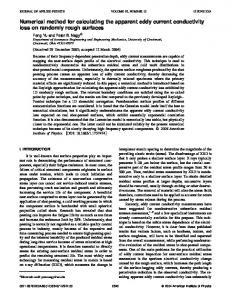
direction. Also, the calculated external inductance in the CST MWS is slightly higher at d.c. than at higher frequencies (∼ 140 MHz), and this difference is around 2%. In Figures 10(a) and (b) the results for the bigger computational domain and d.c. case are shown. All the results of modeling using the CST MWS lie between the curve obtained by MEC, and the curves calculated using SC conformal mapping [41] and approximation in [24]. In the CST MWS, some of the fringing magnetic flux is absorbed by a perfectly matched layer used to limit the computational domain, so the results of computations might be underestimated. In the conformal mapping method the results are underestimated as well, since the width of the trace and thickness of the ground plane are not taken into account. The MEC gives the highest results, since the integration in this method is accomplished in an almost infinitely large space around the microstrip structure. Figure 11 demonstrates by the arrows the magnetic field picture near the microstrip geometry.

Figure 11. CST Microwave Studio modeling of magnetic field near the microstrip geometry with a finite-size ground plane. Figure 12 shows the surface current distributions on the top and the bottom of the ground plane. These figures are obtained using the CST MWS software. The geometry of the structure is the same as discussed above, and the trace is shift by 15 mm from the center of the ground plane. It is seen that there are regions of enhanced surface current on the bottom of the ground plane close to the edges, and it is this current that is responsible for the mutual external inductance of interest.


219

S urface c urre nts TOP View (cas e 1 5 mm s hift) abs va lue

(a)

(b)

Figure 12. CST Microwave Studio modeling of surface current distributions (a) on the top, and (b) on the bottom of the ground plane in a microstrip geometry. It should be mentioned once more that the MEC might overestimate the mutual external inductance for very narrow ground planes, since it considers edge currents distributed evenly only on the rounded edges of the ground plane. As Figure 12 shows, in reality the cut-off “tails” are redistributed on the bottom side of the ground plane, with the current density decreasing exponentially staring from the very edge towards to the center of the ground plane. This may be a direction for the further improvement of the model.

220

Koledintseva et al.

4. CONCLUSION A Method of Edge Currents is proposed for calculating the mutual external inductance associated with fringing magnetic fields in microstrip structures. This method employs a quasi-static (quasimagnetostatic and quasi-TEM) approach, image theory, superposition, and a direct magnetic field integration technique. It is shown that the residue surface currents on the tails that are cut off may be redistributed on the edges of the ground planes of finite thickness. When the ground plane is of zero thickness, these edge currents shrink and become filamentary. It is also shown that the mutual external inductance is determined mainly by the magnetic flux produced by these edge currents, while the contributions to the magnetic flux by the currents from the signal trace and the finite-size ground plane totally compensate each other. This approach has been applied to estimating mutual inductance for both symmetrical and asymmetrical microstrip lines as well. There is a good agreement with published experimental, as well as with full-wave numerical simulations. The practically important conclusion is the following. The results of the presented computations show that, from an electromagnetic immunity (EMI) point of view, it is not acceptable to have a signal trace in a microstrip line closer than 20% of the ground plane width from the edge. This is a general and approximate recommendation for a designer. However, mutual external inductance should be evaluated for every particular case, since it depends on the offset of the signal trace from the center, on the width of the ground plane, height of the transmission line, width of the trace, and the thickness of the ground plane. The presented Method of Edge Currents gives the upper limit (worst case) of the possible mutual inductance associated with fringing magnetic fields. The practical edge values of MEI should be below the values calculated by the present method. This is beneficial for a designer. The resultant MEI is frequency-independent, since the method is limited by the quasi-static consideration, when the TEM mode is the only propagating mode in the structure. The presented approach may also be used for the analysis of striplines and multiconductor planar transmission lines, since it is based on the superposition principle. Generalization for the multimode regime of the wave propagation is also possible. ACKNOWLEDGMENT CST MICROWAVE STUDIO(R) was used in the preparation of this paper under a collaboration agreement between UMR and CST of


221

America, Inc. REFERENCES 1. Wadell, B. C., Transmission Line Design Handbook, Artech House, 1991. 2. Mongia, R., I. Bahl, and P. Bhartia, RF and Microwave CoupledLine Circuits, Artech House, Norwood, MA, 1999. 3. Edwards, T. C. and M. B. Steer, Foundations of Interconnect and Microstrip Design, 3rd edition, Wiley, 2000. 4. Maloratsky, L. G., Passive RF and Microwave Integrated Circuit Design, Elsevier, 2004. 5. Bahl, I. and P. Bhartia, Microwave Solid State Circuit Design, Wiley, 2nd edition, 2003. 6. Kiang, J. F., S. M. Ali, and J. A. Kong, “Modeling of lossy microstrip lines with finite thickness,” Progress In Electromagnetics Research, PIER 04, 85–117, 1991. 7. Takuma, T., Y. Tajima, T. Ichida, A. Z. Elsherbeni, V. RodriguezPereyra, and C. E. Smith, “The effect of an air gap on the coupling between two planar microstrip lines,” Journal of The Franklin Institute, Vol. 333, No. 2, 201–223, March 1996. 8. Watanabe, K. and K. Yasumoto, “Coupled-mode analysis of coupled microstrip transmission lines using a singular perturbation technique,” Progress In Electromagnetics Research, PIER 25, 95–110, 2000. 9. Chai, C. C., B. K. Chung, and H. T. Chuah, “Simple time-domain expressions for prediction of cross-talk on coupled microstrip lines,” Progress In Electromagnetics Research, PIER 39, 147–175, 2003. 10. Khalaj-Amirhosseini, M. and A. Cheldavi, “A new twodimensional analysis of microstrip lines using rigorously coupled multi-conductor strips model,” J. of Electromagn. Waves and Appl., Vol. 18, No. 6, 809–825, 2004. 11. Khalaj-Amirhosseini, M., “Determination of capacitance and conductance matrices of lossy shielded coupled microstrip transmission lines,” Progress In Electromagnetics Research, PIER 50, 267–278, 2005. 12. Arshadi, A. and A. Cheldavi, “Simple and novel model for edged microstrip line (EMTL),” Progress In Electromagnetics Research, PIER 65, 247–259, 2006. 13. Nashemi-Nasab and A. Cheldavi, “Coupling model of the two

222

14.

15.

16.

17.

18.

19.

20.

21.

22.

23.

Koledintseva et al.

orthogonal microstrip lines in two-layer PCB board (Quasi-TEM approach),” Progress In Electromagnetics Research, PIER 60, 153–163, 2006. Khalaj-Amirhosseini, M. and A. Cheldavi, “Wideband and efficient microstrip interconnects using multi-segmented ground and open traces,” Progress In Electromagnetics Research, PIER 55, 33–46, 2005. Ymeri, H., B. Nauwelaers, K. Maex, and D. D. Roest, “New modeling approach of on-chip interconnects for RF integrated circuits in CMOS technology,” Microelectronics International, Vol. 20, No. 3, 41–44, 2003. Van Horck, F. B. M., Electromagnetic Compatibility and Printed Circuit Boards, CIP-Data Library, Technische Universiteit Eindhoven, 1998. Leferink, F., “Inductance calculations: methods and equations,” Proc. 1995 IEEE Int. Symp. Electromagnetic Compatibility, 16– 22, Atlanta, August 14–18, 1995. Hubing, T. H., T. P. Van Doren, and J. L. Drewniak, “Identifying and quantifying printed circuit board inductance,” Proc. 1994 IEEE Int. Symp. Electromagnetic Compatibility, 205– 208, Chicago, IL, USA, Aug. 1994. Hockanson, D. M., J. L. Drewniak, T. H. Hubing, T. P. Van Doren, F. Sha, and C. W. Lam, “Quantifying EMI resulting from finiteimpedance reference planes,” IEEE Trans. Electromagn. Compat., Vol. 39, No. 4, 286–297, Nov. 1997. Ooi, T. H., S. Y. Tan, and H. Li, “Study of radiated emissions from PCB with narrow ground plane,” Int. Symp. Electromagnetic Compatibility, Paper No. 20A101, 552–555, Tokyo, May 17–21, 1999. Hockanson, D. M., J. L. Drewniak, T. H. Hubing, T. P. Van Doren, F. Sha, and M. Wilhelm, “Investigation of fundamental EMI source mechanisms driving common-mode radiation from printed circuit boards with attached cables,” IEEE Trans. Electromagn. Compat., Vol. 38, No. 4, 557–565, Nov. 1996. Holloway, C. L. and G. A. Hufford, “Internal inductance and conductor loss associated with the ground plane of a microstrip line,” IEEE Trans. Electromagn. Compat., Vol. 39, No. 2, 73–77, May 1997. Celozzi, S., G. Panariello, F.Schettino, and L. Verolino, “A general approach for the analysis of finite size PCB ground planes,” Proc. 2000 IEEE Int. Symp. Electromagnetic Compatibility, Vol. 1, 357– 362, Washington DC, Aug. 2000.


223

24. Leone, M., “Design expressions for the trace-to-edge commonmode inductance of a printed circuit board,” IEEE Trans. Electromagn. Compat., Vol. 43, No. 4, 667–670, Nov. 2001. 25. Akdagli, A., “An empirical expression for the edge extension in calculating resonant frequency of rectangular microstrip antennas with thin and thick substrates,” J. of Electromagn. Waves and Appl., Vol. 21, No. 9, 1247–1255, 2007. 26. Yang, F., V. Demir, D. A. Elsherbeni, and A. Z. Elsherbeni, “Enhancement of printed dipole antennas characteristics using semi-EBG ground plane,” J. of Electromagn. Waves and Appl., Vol. 20, No. 8, 993–1006, 2006. 27. Ataeiseresht, R., C. Ghobadi, and J. Nourinia, “A novel analysis of Minkovski fractal microstrip patch antenna,” J. of Electromagn. Waves and Appl., Vol. 20, No. 8, 1115–1127, 2006. 28. Shams, K. M. Z., M. Ali, and H.-S. Hwang, “A planar inductively coupled bow-tie slot antenna for WLAN applications,” J. of Electromagn. Waves and Appl., Vol. 20, No. 7, 861–871, 2006. 29. Kuo, L.-C., H.-R. Chuang, Y.-C. Kan, T.- C. Huang, and C.H. Ko, “A study of planar printed dipole antennas for wireless communication applications,” J. of Electromagn. Waves and Appl., Vol. 21, No. 5, 637–652, 2007. 30. Ren, W., J. Y. Deng, and K. S. Chen, “Compact PCB monopole antenna for UWB applications,” J. of Electromagn. Waves and Appl., Vol. 21, No. 10, 1411–1420, 2007. 31. Eldek, A. A., “Numerical analysis of a small ultrawideband microstrip-fed tab monopole antenna,” Progress In Electromagnetics Research, PIER 65, 59–69, 2006. 32. Ali, M. and S. Sanyal, “A numerical investigation of finite ground planes and reflector effects on monopole antenna factor using FDTD technique,” J. of Electromagn. Waves and Appl., Vol. 21, No. 10, 1379–1392, 2007. 33. Grover, H. W., Inductance Calculations: Working Formulas and Tables, Dover Publications, New York, NY, 1962. 34. Hoer, C. and C. Love, “Exact inductance calculations for rectangular conductors with applications to more complicated geometries,” Journal of Research of the National Bureau of Standards, Vol. 69 C, No. 2, 127–137, 1965. 35. Maxwell, J. C., A Treatise on Electricity and Magnetism, 3rd edition, Oxford University Press, 1892. 36. Kaden, H., Wirbelstroeme und Schirmung in der Nachrichtentechnik. Technische Physik in Einzeldarstellungen Herausgegeben, von

224

37.

38. 39.

40.

41.

42.

43.

44.

45.

Koledintseva et al.

W. Meissner (ed.), 2nd edition, 262–282, Springer-Verlag, Berlin, Germany, 1959. Ruehli, A. E., “Inductance calculations in a complex integrated circuit environment,” IBM Journal on Research and Development, Vol. 16, No. 5, 470–481, Sept. 1972. Carson, J. R., “Wave propagation in overhead wires with ground return,” Bell Syst. Techn. Journal, Vol. 5, 539–554, 1926. Kobayashi, M., “Longitudinal and transverse current distributions on microstriplines and their closed-form expression,” IEEE Trans. Microwave Theory and Techn., Vol. 33, No. 9, 784–788, 1985. Holloway, C. L. and E. F. Kuester, “Closed-form expressions for the current density on the ground plane of a microstrip line, with application to ground plane loss,” IEEE Trans. Microwave Theory and Techn., Vol. 43, No. 5, 1204–1207, May 1995. Van Horck, F. B. M., A. P. J. van Deursen, and P. C. T. van der Laan, “Common-mode currents generated by circuits on a PCB — Measurements and transmission-line calculations,” IEEE Trans. Electromag. Compat., Vol. 43, No. 4, 608–617, Nov. 2001. Holloway, C. L. and E. F. Kuester, “Closed-form expressions for the current densities on the ground planes of symmetric stripline structures,” IEEE Trans. on Electromagn. Compat., Vol. 49, No. 1, 49–57, Feb. 2007. Vaidyanath, A., B. Thoroddsen, J. L. Prince, and A. C. Cangellaris, “Simultaneous switching noise: influence of plane-plane and plane-signal trace coupling,” IEEE Trans. on Advanced Packaging, Vol. 18, No. 3, 496–502, Aug. 1995. Berg, D., M. Tanaka, Y. Ji, X. Ye, J. L. Drewniak, T. H. Hubing, R. E. DuBroff, and T. P. Van Doren, “FDTD and FEM/MOM modeling of EMI resulting from a trace near a PCB edge,” Proc. IEEE Int. Symp. Electromagnetic Compatibility, 135–140, Washington, DC, Aug. 2000. Watanabe, T., O. Wada, Y. Toyota, and R. Koga, “Estimation of common-mode EMI caused by a signal line in the vicinity of ground edge on a PCB,” Proc. of IEEE Int. Symp. Electromagnetic Compatibility, Vol. 1, 113–118, Minneapolis, MN, Aug. 2002.