2013 IEEE 9th International Conference on e-Science
Mining Common Spatial-temporal Periodic Patterns of Animal Movement Yuwei Wang∗† , Ze Luo∗ , Gang Qin∗ , Yuanchun Zhou∗ , Danhuai Guo∗ and Baoping Yan∗ ∗ Computer Network Information Center Chinese Academy of Sciences, Beijing, China Email:
[email protected] † University of Chinese Academy of Sciences, Beijing, China Email:
[email protected]
data collection [4]. First, the periodicity is inaccurate. It is impossible that the object repeat the same location w.r.t. the period. Usually, in order to solve the ambiguity of the location, the geospatial space is divided and movement data is transformed into symbol sequence [1], [5] depending on whether or not the location is in the corresponding region. Then, traditional period detection methods designed on time series are used, such as Fast Fourier Transform (FFT) and auto-correlation [3]. Second, the irregularity exists in the GPS data collection process due to the limitations of GPS devices and other interferences, such as bad weather. There exist a large number of missing data [4], and the sampling intervals between continuous observations are uneven which vary from several minutes to several days. The imperfect data collection further increases the complexity of period detection, so that traditional methods cannot be applied directly [4]. To address the second problem mentioned above, a probabilistic model of incomplete observations and a novel periodicity measure are proposed to detect the event period in a long sequence in [4]. However, in animal tracking scenes, GPS data is usually acquired in a limited lifespan due to the equipment energy constraint. For example, the lifespan of GPS data from a bird is usually less than 2 years in the migratory bird tracking in Qinghai Lake, China [6], [7]. Data missing with random time length may occur in random moment due to occasional equipment failure. Besides, individuals may follow different periodic patterns in different cycles. Owing to individual uncertainty, the time span to stay in a single region often shifts in different cycles. Previous periodicity analysis methods which usually considers the periodicity against a single region are hard to deal with the periodicity discovering problem on individual data with the very limited time length. Even though some weak periods of some individuals can be detected in some region, a big divergence may exist among the results even though individuals follow the same periodicity. In this paper, we formulate the common spatial-temporal periodicity problem, and propose corresponding methods at several stages to address the problem. The proposed methods overcome aforementioned issues caused by the limitation in data collection and uncertainty in individual behaviors.
Abstract—Advanced satellite tracking technologies enable biologists to track animal movements at finer spatial and temporal scales. The resulting long-term movement data is very meaningful for understanding animal activities. Periodic pattern analysis can provide insightful approach to reveal animal activity patterns. However, individual GPS data is usually incomplete and in limited lifespan. In addition, individual periodic behaviors are inherently complicated with many uncertainties. In this paper, we address the problem of mining periodic patterns of animal movements by combining multiple individuals with similar periodicities. We formally define the problem of mining common periodicity and propose a novel periodicity measure. We introduce the information entropy in the proposed measure to detect common period. Data incompleteness, noises, and ambiguity of individual periodicity are considered in our method. Furthermore, we mine multiple common periodic patterns by grouping periodic segments w.r.t. the detected period, and provide a visualization method of common periodic patterns by designing a cyclical filled line chart. To assess effectiveness of our proposed method, we provide an experimental study using a real GPS dataset collected on 29 birds in Qinghai Lake, China. Keywords-animal movement; spatial-temporal data; common periodic pattern; information entropy;
I. I NTRODUCTION With the rapid development of satellite tracking technologies and the popularity of mobile devices in recent years, massive movement data from various moving objects, such as animals, humans, and cars, have become available. The movement data have played a significant role in investigating movement behaviors at finer spatial and temporal scale. Many data mining approaches have been applied on the movement data to reveal activity patterns of moving objects. The activities of moving objects often present some periodicity. They follow similar routes over regular temporal intervals [1]. For example, a person often follows a same activity sequence daily or weekly, migratory animals usually follow similar migration trajectories yearly. Mining periodic behaviors hidden in the spatial-temporal data provide us with insightful information of the activities [2], [3]. In many real applications, discovering unknown period and corresponding periodic patterns is very challenging owing to ambiguity of periodicity and incompleteness of 978-0-7695-5083-1/13 $25.00 © 2013 IEEE DOI 10.1109/eScience.2013.11
17
First, we detect the common habitats using modified kernel density estimation and spatial clustering approach. With respect to these habitats, we transform the spatial-temporal data into multi-symbol time series. Second, we propose a new measure for common periodicity. The measure is based on an observation that the data distribution of all individuals is highly skewed in most of time instances w.r.t. the true period. We use information entropy to measure this characteristic and thus determine the true period. Third, we use clustering approach to mine multiple common periodic patterns. Fourth, we design a cyclical filled line chart and coordinate it with a space-time view to visualize the spatialtemporal patterns. The main contributions of our work are: (1) We propose common periodicity of individuals and formally define the problem of common spatial-temporal periodic periodicity; (2) We propose a novel periodicity measure to detect the common periodicity; (3) We extend exiting periodic pattern mining method to mine multiple common periodic patterns; (4) We design a visualization view to convey the spatialtemporal common patterns. The rest of the paper is organized as follows. Section 2 discusses related work. Section 3 formally defines the common periodicity detection problem and provides solutions. Section 4 presents our experimental results. Finally, Section 5 summarizes this paper.
sum of the distances between the trend and all segments are minimized. To calculate the distance faster, a segment denoted as a symbol vector is mapped to a sketch vector in fewer dimensions. The map preserves good approximation of the distance between two sketch vectors to original distance between the segments, meanwhile reducing the computational complexity. In [11], the first segment is chosen as candidate trend in the sequence, so effectiveness of the detected periodicity is strongly dependent on the beginning of the sequence. The method can only detect the most significant periodicity. Due to noise and imperfection of periodicity, each element in the pattern may have a phase shift in the sequence. [12] accounts for the problem by including a time tolerance δ. In [12], a periodic pattern is defined as a periodic temporal association rule in which the relative order of events is not cared. The input is an uneven time series and the distribution of the intervals between adjacent occurrences is computed. The distribution is considered to be bigger at the potential period than at other interval values. However, [12] has an obvious drawback as depicted in [13], i.e., only the intervals between adjacent occurrences are treated as candidates and this leads to missing of some true periods. [14] considers another form of disturbance: misalignment of a pattern in event sequence caused by random insertion of noise events. They have proposed an algorithm to detect this asynchronous periodic pattern and its longest valid subsequence. The valid subsequence is formed in two steps under the control of two parameters: min rep and max dis. A valid subsequence is a set of successive valid segments in which the disturbance between segments is not greater than max dis [14], while a valid segment requires min rep repetitions of non-disrupted pattern occurrences. They maintain a moving window, and use the frequent adjacent intervals of a symbol in the window as candidate periods of the symbol. Hence, [14] has the similar drawback of missing some periods as [12]. A convolution-based algorithm with two mapping schemes is proposed in [13] to detect two kinds of periodicities (symbol periodicity and segment periodicity). Symbol period detection aims to discover the periods of each symbol. Segment periodicity concerns the periodicity throughout entire series in which the whole segments is periodic. The periodicity measure in [13] is the same as auto-correlation [15] essentially. [16] converts the time series into binary vector w.r.t. each symbol and then finds the periods using auto-correlation and FFT. Additionally, [16] extends period detection method to capture approximate periodicity. An approximate periodic instance, in which some elements are shifted or missed, would be included into the frequency of the pattern with a weight relative to its degree of deformation. Usually, spatial-temporal periodic pattern mining is converted into time series mining problem by geospatial division along with mining [1], [5] or prior to mining [3]. Due to
II. R ELATED W ORK There has been a lot of work concerning periodicity in time series. These studies usually address the periodicity in the case of the input is a symbol sequence or in the case of time series is transformed to a symbol sequence by categorizing the real value [4]. The original or the processed sequences only retain the relative order of events instead of real time, in which a symbol represents an occurrence of an event. The periodicity is determined based on the support of the pattern. Given the period T and the symbol sequence, [8] has proposed the problem of partial periodic pattern: only a part of time units in the pattern have periodicity. They define the pattern as V0 , V1 , · · · , VT −1 where Vi (0 ≤ i < T ) is an event symbol or a wildcard * which matches any event [8]. The pattern is segment-wise (i.e., it does not have to repeat in all segments).They consider the support of a pattern as the ratio of the segments which match the pattern exactly in the entire sequence. A pattern with k non-wildcard symbols is named k-cycle pattern, and Apriori principle [9] is utilized to find level-wise patterns. A max-subpattern hit set property is exploited in [10] for computing the supports of these patterns faster. A max-subpattern tree structure is designed in [10] to count the occurrences of all possible patterns, so that only two database scans are needed even for multiple periods. Given a symbol sequence and a periodic range, [11] finds the most significant periodic trend in the sense that the 18
the lack of predefined spatial regions, [5] discovers frequent periodic patterns and corresponding regions automatically and simultaneously from spatial-temporal data with a given period T . It imposes a constraint that the set of i-th locations in the segments complying with a pattern V0 , V1 , · · · , VT −1 forms a dense spatial cluster if Vi (0 ≤ i < T ) is not a wildcard. [5] defines pattern length as the number of nonwildcard elements, and designs a pattern growth algorithm to mine longer patterns step by step. [1] extends this work to exploit the pattern occurrences of whose elements in a pattern instance may be shifted or distorted within a predefined time threshold δ. The problem is addressed by duplicating a point to all neighbor positions. In addition, they search validity eras of a pattern, which are the time spans in which the pattern keeps frequent. [2] has proposed a problem of discovering period from a trajectory of a moving object. They first transform the locations to displacement vectors in the complex plane w.r.t. the starting location, and generate the periodogram using Complex Fourier Transform (CFT). The periodogram indicates that a period exists at a significant peaks [2]. However, the method is sensitive to noise in the path, and inapplicable on complicated movement data with a lot of spatial noise [3]. [3] has proposed a two-stage framework to address problems of period detection and pattern mining. Reference spot is used to transform the movement data to a binary sequence. FFT and auto-correlation methods are used to detect periods for a spot. Then, the spots with the same period are considered together, and the periodic behavior is modeled as a generative model. Multiple periodic behaviors with the same period can be discovered using a hierarchical clustering method. Incompleteness in GPS data collection is a common phenomenon. A large number of missing data increase the difficulty of period detection using traditional methods such as FFT and auto-correlation. To overcome the problem, [4] models periodicity of incomplete observations of an event as a probabilistic model and provides a periodicity measure based on the observation that the occurrences of the event converge in some specific intervals after overlaying the data using the true period. Hence, they measure the periodicity using the discrepancy between probabilities of occurrence and nonoccurrence of the event in these intervals relative to the periodic length. All works above deal with periodicity of a time series or a spatial-temporal trajectory from an individual over a history long enough relative to the period. These works only exploit the periodicity w.r.t. a single symbol or a single region. However, in animal tracking scenes, GPS data is usually acquired in a limited lifespan and has a large number of missing. The periods detected by previous methods on the individual and w.r.t. a region may have big divergences even though the underlying periodicity is the same essentially. Multiple animals tracked in an application usually follow the same
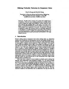
periodicity. In this case, considering common periodicity of multiple individuals during the entire cycle can compound the uncertainty in individual periodic behaviors. Different from previous works, our method aims to detect periodicity that is followed concurrently by multiple individuals by mining from individual insufficient movement sequences in a mutual reinforcement manner. III. M INING C OMMON P ERIODICITY A. Problem Definition Assume that a movement database D = {D1 , D2 , . . . , Dd } is collected from d objects, and Dk = {⟨l1k , tk1 ⟩, ⟨l2k , tk2 , ⟩, . . .} is the spatial-temporal data of k-th object in ascending order of timestamp t in which l1k is the location at timestamp tk1 . The data from different objects have different lifespans and uneven sampling intervals. Without loss of generality, assume that the minimum timestamp in D is 0 and the maximum timestamp is dur. We consider the similarity of generated movement segment sets L1 , L2 , . . . , LN , (N = ⌈dur/T ⌉) after slicing D w.r.t. time length T . L1 , L2 , . . . , LN start after 0, T, 2T, . . . , (N − 1) · T respectively, and Li is the set of movement segments {Di1 , Di2 , . . . , Did } from all individuals where Dik = {⟨l, t⟩ | ⟨l, t⟩ ∈ Dk , i · T ≤ t < (i + 1) · T } (1 ≤ k ≤ d, 1 ≤ i ≤ N ). Our problem is mining common periodicity, including the period length T , the periodic pattern set {P1 , P2 , . . .} w.r.t. T and the movement segments complying with each pattern. We define the common periodicity as follows. Definition 1. Given a movement database D from d objects and maximum timestamp dur. If there exists an time length T ∈ R+ , 0 < T < dur, such that when we slice D into segment sets L1 , L2 , . . . , LN , the sets Li , Lj are similar for all i and j (1 ≤ i ≤ N, 1 ≤ j ≤ N, N = ⌈dur/T ⌈). We say D has a common periodicity, and T is the common period. We first try to detect period on a single object and single region according to [3]. However, due to the data missing and limited time length, the period can be hardly detected. As illustrated in Fig. 1, these objects have a common periodicity with period 5. Consider a unique region on any object, the periodicity is obscure. In addition, due to the diversity in individuals, we would get a lot of regions (namely habitats in the rest of the paper). There is some intrinsical similarity among these habitats, for example, several individual habitats may belong to a common large habitat of the species essentially. Hence, we consider the common habitats instead of individual habitats for common periodic pattern detection. In Fig. 1, individual habitats have been combined, and symbols with identical color denote a common habitat. Let an alphabet Σ = {−1, 0, 1, . . .} represent the identifier set of common habitats, in which -1 denotes any region outside of all habitats. We replace the exact location in D, 19
Figure 1.
account for predefined percentage of the distribution volume, and 95% is often used as the suitable percentage [17], [18], [19]. Various kernels have been developed, such as bivariate normal kernel, Epanechnikov kernel, and biweight kernel [21]. According to [20], [22], different kernels result in extremely similar distributions. Here, we use the biweight kernel [21]: { 3 (1 − uT u)2 uT u < 1, (2) k(u) = π 0 otherwise.
An illustration example of movement time series of 5 objects.
The smoothing parameter h is a critical factor of the estimate, because that a large value of h would oversmooth the data while a small value would overfit and produce false ”peaks” [19], [23] in sparse regions. Hence, we use KDE with variable smoothing parameter [21], [23]:
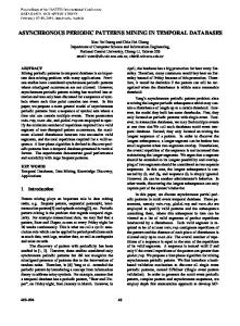
and get a multi-symbol time series for each object. If D has a common period T0 , the locations {ltk | t ≤ (tki mod T ) ≤ t + 1, 1 ≤ k ≤ d} at any relative interval t (0 ≤ t < T0 ) with a predefined time granularity w.r.t T0 should converge in a minority of the habitats. Hence, the distribution of Σ would be skewed on the corresponding symbol collection. As suggested by Fig. 2a, when we use the true period T = 5 to slice the data in Fig. 1 with time granularity 1, and get segment sets L1 , L2 , L3 , L4 , we can see that the distribution is highly skewed at most of the time t (0 ≤ t < 5) except t = 4 ( it implies multiple common patterns actually). When T = 4, the distribution at each time t (0 ≤ t < 4) tends to be uniform, as shown in Fig. 2b. We characterize this characteristic by introducing a concept from information theory, and thereby propose a measure for period detection.
1∑ 1 d(x, xi ) K( ), n i=1 h2i hi n
f (x) =
(3)
where hi is the smoothing parameter at the observation xi . Usually, hi is set as the distance from xi to its k-nearest spatial neighbor. Because the activity scale of an animal varies in different stages, the influence of an observation should vary with current activity scale. Thus, we adjust hi relative to temporal neighbors of xi by maintaining a sliding time window W , and set hi as the furthest distance in current window: hi = max(h, d(xi , xj )), where xj ∈ N eri , and (4) |W | N eri = {x | ⟨x, t⟩ ∈ Dk , |ti − t| ≤ }. 2 We set a minimum of smoothing parameter [23] to avoid nearly zero in the case of an animal stays at the same location or very proximate locations, or only an observation exists in the window. The data incompleteness and unevenness lead to the deviation of the estimation that relatively high density emerges in more sampled region while relatively low density in the region where the sampling frequency is low. Assigning different weights to observations can weaken interference of data incompleteness on the results [24]. Thus, the weight of an observation should depend on the data frequency around the observation time. Here, we define the weight of an observation as inversely proportional to the exponent of the number of observations in current time window: wi = e1−|N eri | (5)
B. Common Habitat Detection Many methods have been proposed to identify animal habitats, such as Minimum Convex Polygon (MCP), Kernel Density Estimation (KDE) [17] and spatial clustering [6]. We adopt KDE owing to its insensitivity to noise and good efficiency. KDE is proposed for estimating animal home range in 1989 [18], and has been widely used as animal utilization distribution estimator [17], [19]. KDE models the influence of each observation (the location in GPS data) to the data space as a kernel function, which is a probability density function and usually nonincremental w.r.t. the distance. The density of a location is defined as the average influence of all observations to this location. Given a two dimensional dataset with size n, the density at location x is defined as follows according to [18], [20]: n d(x, xi ) 1∑ 1 K( ), (1) f (x) = 2 n i=1 h h
The habitats of individuals interconnect intrinsically. We cluster the habitats of all individuals to form common habitats automatically. The common habitats reduce the ambiguity of individual behaviors. We identify automatically the clustering structure using OPTICS algorithm [25], and further cluster the habitats using DBSCAN algorithm [26] with auxiliary parameter determination from OPTICS. An
where h denotes smoothing parameter, K(·) is the kernel function, and d(x, xi )is the distance between x and an observation xi . A density surface is generated which denotes the probability that an animal appears at any location. Habitats usually are output as the smallest regions which 20
(a) Figure 2.
(b)
The distribution of Σ after overlaying and combining the data in Fig. 1 w.r.t candidate period T . (a) T = 5. (b) T = 4.
from {S1 , S2 , . . . , SN } within the interval. For the example in Fig. 1 and T = 5, the symbol collection of 0−th inteval s0 is {0(8), −1(2)} where 8 and 2 in brackets are frequencies of symbol 0 and -1. Thus, a frequency histogram series is generated w.r.t. T , as shown in Fig. 2. Further, we normalize the frequency histogram in t-th interval (0 ≤ t < T ). Observe the normalized histogram series from interval 0 to interval T −1. The distribution p(st ) is highly skewed (i.e., all objects prefer a minority of the habitats) at most of the intervals for the true period T0 while more uniform for other candidates. Information entropy [27] can be used to quantify this distribution characteristic: |Σ|−2
Et (S) = −
∑
p(st = i) log p(st = i),
(7)
i=−1
Figure 3.
Thus, we define the negative measure for candidate period T as: T −1 ∑ E(T ) = − Et (S). (8)
Common habitats of multiple individuals.
t=0
example is shown in Fig. 3 where outer polygons are common habitats and small color-filled polygons are individual habitats. After obtaining the common habitat set C = C0 , C1 , . . ., the movement data Dk is transformed to multi-symbol time series S k = ⟨s(l1k , C), tk1 ⟩, ⟨s(l2k , C), tk2 ⟩, . . . according to: { i Ci contains l, s(l, C) = (6) −1 otherwise,
If the function E(T ) (1 < T < dur) is concave in some range and has local minimum at T0 in the range, it suggest T0 is a common period of D. Note that multiple local minimums indicate multiple period exist in D. D. Mining Common Periodic Patterns After detecting the period T0 , we need to mine common periodic patterns and the movement segments corresponding to each pattern. Multiple patterns may exist in the movement database. For example, two patterns ⟨0, 0, 1, 3, 2⟩ and ⟨0, 0, 2, 3, 2⟩ are located in the example in Fig. 1. Like the pattern definition in [3], the common periodic pattern is also denoted as a two-dimensional probability matrix P whose element Pi t is the probability that the group of individuals complying with the pattern emerge in the region i at time t (0 ≤ t < T0 ). Let S(P ) denote the set of period segments complying with P from {S1 , S2 , . . . , SN }. We call the element in S(P ) is a valid segment of P . Note that the segments from an individual may belong to different patterns due to animal behavior may shift over different cycles.
Now, our problem is converted to common periodicity of multi-symbol time series database. C. Common Period Detection For a multi-symbol time series database S = {S 1 , S 2 , . . . , S d }, we slice the series w.r.t a candidate period T , the generated segment sets {S1 , S2 , . . . , SN } where Si = {Si1 , Si2 , . . . , Sid } and Sik = {⟨s, t⟩ | ⟨s, t⟩ ∈ S k , i·T ≤ t < (i + 1) · T }. The resulting sets will present a high degree of regularity when T is the true period. Let t (0 ≤ t < T ) be tth interval w.r.t. T and st be the symbol collection obtained 21
[3] uses a clustering approach with Kullback-Leibler (KL) distance metric to group the periodic behaviors. We extend this method to address the problem of common periodic pattern mining. By clustering, the segments complying with different patterns will be divided into different groups. A distance function between the segments needs to be defined. A segment corresponds to a frequency histogram series described above. The distance computation methods of histograms such as Euclidean distance, chi-square coefficient, and Bhattacharyya distance [28] can be used to define the segment distance. Here, we use Bhattacharyya distance to measure the distance instead of KL distance due to nonsymmetry of KL distance: v |Σ|−2 T −1 u u ∑ √ ∑ t1 − d(S1 , S2 ) = p1 (st = i)p2 (st = i). (9) t=0
Figure 4. Cyclical filled line charts for two patterns in a region with period T0 = 365.
space through the spatial-temporal and circular graphical encoding. In the cyclical filled line chart, the probability matrix of a pattern is encoded in a polar coordinate system. A row of the probability matrix which describe the periodicity relative to the corresponding habitat, is shown as a ring chart. The ring is the metaphor of the periodicity. The radius of the ring is proportional to the cluster size of the pattern. The angle represents the time dimension in the probability matrix. The distance from the center to the point at some angle represents the probability in corresponding time. Each element in the row is drawn as a point in the polar coordinate system. The points are connected by a polyline, and then the cyclical polyline is filled with a unique color associated with the pattern. The different rows in the pattern matrix are represented by different charts, and are linked to different habitats. By differently coloring the patterns we provide an easy distinguishability therebetween. The color for a pattern is used to color the pattern in the cyclical filled line chart, and the segment paths complying with the pattern in spacetime view. This provides a direct linkage between the pattern summarization and the pattern instances. Fig. 4 is an example of two patterns with same period T0 = 365. An obvious difference exists from time 150 to time 240.
i=−1
Some parts of segments may be shifted due to ambiguity of periodic behavior or contingency of individual behavior. In addition, there exist many missing data and noise. To handle these difficulties, we duplicate the location along its time window of size ε with non-increasing weight function Φ(·). Therefore, the probability that an individual is in region i is deformed as: t+ε ∑
p¯(st = i) =
Φ(|k − t|) · 1i (sk )
k=t−ε |Σ|−2 ∑
t+ε ∑
,
(10)
Φ(|k − t|) · 1j (sk )
j=−1 k=t−ε
where 1j (s)(i ∈ Σ) is the indicator function such that the 1j (s) = 1 if and only if s = i. Similar to common habitat clustering, the clustering structure and number of patterns can be identified automatically using OPTICS algorithm. Once the segment clusters are formed, the common periodic patterns can be generated by summarizing the clusters [3]. We collect the normalized histogram series of the segments belonging to the same cluster. Further, we average the histograms in the corresponding interval, and a twodimensional probability matrix is output for a pattern. The periodic patterns could be visualized in space-time view by integrating the temporal and quantitative characteristics of the pattern matrix, and the spatial characteristics of the habitats.
IV. E XPERIMENTAL STUDY In this section, we systematically evaluate various aspects of our proposed methods and present the experimental results on a real movement dataset collected from wild birds. A. Experimental Dataset
E. Pattern Visualization
We use a real GPS dataset of 29 Bar-headed Geese tracked from March 2007 to January 2010 in Qinghai Lake National Nature Reserve, Qinghai province, China. 29 Bar-headed Geese were equipped with GPS solar-powered Platform Terminal Transmitters (PTT; Microwave Telemetry, Columbia, Maryland, USA). The locations were estimated by Argos system and were classified into seven kinds of precisions, or were estimated by GPS. The precision of the location varies from tens of meters to several kilometers. The devices
A simple method to visualize the periodic patterns is using a series of histograms or a bar chart. A problem is that the method cannot represent continuous cyclical nature of the periodic patterns intuitively. Hence, we design a cyclical filled line chart to represent the periodicity. It is linked with a view of space-time cube to represent spatial and temporal characteristics of the movement data and the patterns. Users can easily understand the underlying periodicity in time and 22
were designed to record locations every 2 hours. However, they were unstable so that the recording interval varies from several minutes to ten days. After removing duplicates, 61002 records are remained. Only three movement series last for more than 2 years. A more detailed description of the dataset can be seen in [6], [7]. B. Common Period Detection on Bird Dataset We examine our period detection method on the Barheaded Goose dataset. Bar-headed Goose has annual migratory period, so we can assess the effectiveness of our proposed method by comparing our results with the year period. As shown in Fig. 3, five common habitats along Qinghai-Tibet Plateau are detected by applying detection method in Section 2 on 29 birds. We compare our method with the auto-correlation method in which individual movement series are combined and preprocessed by sampling the symbols daily as the symbol with maximum frequency. An important criterion is the accuracy of the discovered periods. The accuracy depends on the number of the individual and the data completeness. Hence, we test our method under various settings by tuning the number of d, and the sampling rate α with which the data in some day is retained. We define the relative accuracy as: max((15−|T −365|)/15, 0), which means that a completely unsuccessful detection occurs when the detected period T is outside of [350, 380]. Each experiment is repeated 20 times and the average accuracy is reported. First, we tune d from 1 to 25 and set α = 1, and in each setting d birds are sampled from 29 birds. The results are shown in Fig. 5a. The results show that our method outperforms the auto-correlation method for different number of individuals. The accuracy of our method reaches 82.5% (i.e., the difference between our detected period and the true period is about 2 days) when d = 10. When d = 1, the period is barely detected. This explains the need of considering common periodicity of multiple individuals instead of individual period. Second, we assess the accuracy w.r.t. the sampling rate α to measure the impact of missing data. We tune α from 0.2 to 1, and fix d = 29. As shown in Fig. 5b, our method is significantly better than auto-correlation under varying sampling rate. Fig. 6 shows the negative periodicity measure generated by our period. It indicates an obvious period at T0 = 367 and second period T1 = 731 (about 2 · T0 ). Our method prefers the shorter true period T0 = 367 which is more representative than its multiple [4], [13], and helps to remove duplicated period T1 = 731.
Figure 6. birds.
Negative periodicity measure generated by our method on 29
clustering using DBSCAN. We set the distance threshold to 150, and set the minimum number of neighbors of core point MinPts as 4 in OPTICS. The segments whose data last for less than 100 days are filtered out. The generated cluster structure is shown in Fig. 7, in which two clusters are visible.
Figure 7. The clustering structure of movement segments generated by OPTICS algorithm.
According to Fig. 7, we set the core distance parameter of DBSCAN [26] to 100 and apply the algorithm on the segments. Two clusters are obtained both sizes of which are 9, as shown in Fig. 8. We can see that the difference mainly concentrated in the time when birds leave Habitat 1 (Zhaling-Eling Lake, a stopover site) and arrive Habitat 2 (Qinghai Lake, a breeding ground). We visualize the probability matrixes in cyclical filled line chart to further exploit two common periodic patterns. From Fig. 9, we find that these two patterns are similar in Habitat 0 (QinghaiLhasa Valley, a wintering ground), a pattern pass through Habitat 3 (Zhamucuo Wetland, a stopover site) while another pattern does not pass through Habitat 3, and both patterns do not involve Habitat 4 (Hala Lake, a breeding ground). Both patterns start in Habitat 2 around about March 25. However, the birds in pattern 1 leave Habitat 2 from June 10 while the birds in pattern 2 continue to stay in the habitat until late
C. Common Periodic Patterns on Bird Dataset Now we mine periodic patterns from bird dataset. We first segment all movement series of 29 birds w.r.t. T0 = 365. Then, we apply OPTICS [25] to generate clustering structure in order to obtain suitable parameters of subsequent 23
(a)
(b)
Figure 5. Accuracy comparison between our method with auto-correlation method.(a) Accuracy w.r.t. the number of individuals. (b) Accuracy w.r.t data sampling rate.
Figure 8. Two clusters of common period segments in the space-time view in which time is represented by the altitude.
Figure 9. chart.
August. This leads to an obvious difference on the length of time to stay in Habitat 1 because that the departure time in Habitat 1 is similar. The detail of two patterns in the Habitat 2 is shown in Fig. 4. The results indicate that most of Bar-headed Geese follow similar spatial-temporal migratory routes during the whole year, and the main difference in the major routes is the migration time around Qinghai Lake. This experimental study on the real migration data shows the practicality of our method on common periodicity mining and the capability of providing an insightful and intuitive explanation for animal common behaviors. Hence, this approach offers biologists an opportunity to studying the patterns of species which has collective periodic behavior, such as African wildebeests and Ruddy Shelduck.
groups of moving objects. We formally define the problem of common spatial-temporal periodic pattern mining and address the problem in several steps. We first detect the common habitats from the movement data and transform the data to multi-symbol time series. Second, we propose a novel measure for common periodicity based on information entropy. Then, a clustering approach is used to mine common periodic behaviors w.r.t. the period detected in the previous step. Last, we design a spatial-temporal visualization method to represent intuitively the spatial-temporal and cyclical characteristic of the patterns using cyclical filled line chart and space-time cube. An experimental study on real bird dataset proves the need of detecting period from multiple objects, validates the accuracy of our method, and shows the practicality of our method on common periodicity mining and visualization. Our method benefits biologists to understand animal collective behaviors in an insightful and intuitive way. Hence, this work actually provides a potential approach for biologists to
V. C ONCLUSION In this paper, we have proposed the idea of detecting periodicity on imperfect collected movement data from 24
Two common periodic patterns shown in cyclical filled line
study the movement of species which has collective periodic behavior. In future, we consider extending the common pattern to the work of discovering relationships among the individuals of the same species and cross-species.
[8] J. Han, W. Gong, and Y. Yin, “Mining segment-wise periodic patterns in time-related databases,” in Proceedings of the 4th International Conference on Knowledge Discovery and Data Mining, 1998, pp. 214–218. [9] R. Agrawal and R. Srikant, “Fast algorithms for mining association rules,” in Proceedings of the 20th International Conference on Very Lage Databases, vol. 1215, 1994, pp. 487–499.
ACKNOWLEDGMENT Funding was provided by the Natural Science Foundation of China under Grant No. 90912006; The National R&D Infrastructure and Facility Development Program of China under Grant No. BSDN2009-18; The Natural Science Foundation of China under Grant No. 61003138; United States Geological Survey (Patuxent Wildlife Research Center, Western Ecological Research Center, Alaska Science Center, and Avian Influenza Program); the United Nations FAO, Animal Production and Health Division, EMPRES Wildlife Unit; National Science Foundation Small Grants for Exploratory Research under Grant No. 0713027). The use of trade, product, or firm names in this publication is for descriptive purposes only and does not imply endorsement by the U.S. Government.
[10] J. Han, G. Dong, and Y. Yin, “Efficient mining of partial periodic patterns in time series database,” in Proceedings of the 15th International Conference on Data Engineering. IEEE, 1999, pp. 106–115. [11] P. Indyk, N. Koudas, and S. Muthukrishnan, “Identifying representative trends in massive time series data sets using sketches,” in Proceedings of the 26th International Conference on Very Large Databases, 2000, pp. 363–372. [12] S. Ma and J. L. Hellerstein, “Mining partially periodic event patterns with unknown periods,” in Proceedings of the 17th International Conference on Data Engineering. IEEE, 2001, pp. 205–214.
R EFERENCES
[13] M. G. Elfeky, W. G. Aref, and A. K. Elmagarmid, “Periodicity detection in time series databases,” IEEE Transactions on Knowledge and Data Engineering, vol. 17, no. 7, pp. 875– 887, 2005.
[1] H. Cao, N. Mamoulis, and D. W. Cheung, “Discovery of periodic patterns in spatiotemporal sequences,” IEEE Transactions on Knowledge and Data Engineering, vol. 19, no. 4, pp. 453–467, 2007.
[14] J. Yang, W. Wang, and P. S. Yu, “Mining asynchronous periodic patterns in time series data,” in Proceedings of the 6th ACM SIGKDD International Conference on Knowledge Discovery and Data Mining. ACM, 2009, pp. 275–279.
[2] S. Bar-David, I. Bar-David, P. C. Cross, S. J. Ryan, C. U. Knechtel, and W. M. Getz, “Methods for assessing movement path recursion with application to african buffalo in south africa,” Ecology, vol. 90, no. 9, pp. 2467–2479, 2009.
[15] M. Vlachos, P. Yu, and V. Castelli, “On periodicity detection and structural periodic similarity,” in Proceedings of the SIAM International Conference on Data Mining, 2005, pp. 449–460.
[3] Z. Li, B. Ding, J. Han, R. Kays, and P. Nye, “Mining periodic behaviors for moving objects,” in Proceedings of the 16th ACM SIGKDD International Conference on Knowledge Discovery and Data Mining. ACM, 2010, pp. 1099–1108.
[16] C. Berberidis and I. Vlahavas, “Mining for weak periodic signals in time series databases,” Intelligent Data Analysis, vol. 9, no. 1, pp. 29–42, 2005.
[4] Z. Li, J. Wang, and J. Han, “Mining event periodicity from incomplete observations,” in Proceedings of the 18th ACM SIGKDD International Conference on Knowledge Discovery and Data Mining. ACM, 2012, pp. 444–452.
[17] R. A. Powell, “Animal home ranges and territories and home range estimators,” Research techniques in animal ecology: controversies and consequences. Columbia University Press, New York, NY, USA, pp. 65–110, 2000.
[5] N. Mamoulis, H. Cao, G. Kollios, M. Hadjieleftheriou, Y. Tao, and D. W. Cheung, “Mining, indexing, and querying historical spatiotemporal data,” in Proceedings of the 10th ACM SIGKDD International Conference on Knowledge Discovery and Data Mining. ACM, 2004, pp. 236–245.
[18] B. J. Worton, “Kernel methods for estimating the utilization distribution in home-range studies,” Ecology, vol. 70, no. 1, pp. 164–168, 1989. [19] K. M. Berger and E. M. Gese, “Does interference competition with wolves limit the distribution and abundance of coyotes?” Journal of Animal Ecology, vol. 76, no. 6, pp. 1075–1085, 2007.
[6] M. Tang, Y. Zhou, J. Li, W. Wang, P. Cui, Y. Hou, Z. Luo, F. Lei, and B. Yan, “Exploring the wild birds migration data for the disease spread study of h5n1: a clustering and association approach,” Knowledge and Information Systems, vol. 27, no. 2, pp. 227–251, 2011.
[20] D. E. Seaman and R. A. Powell, “An evaluation of the accuracy of kernel density estimators for home range analysis,” Ecology, vol. 77, no. 7, pp. 2075–2085, 1996.
[7] D. J. Prosser, P. Cui, J. Y. Takekawa, M. Tang, Y. Hou, B. M. Collins, B. Yan, N. J. Hill, T. Li, and Y. Li, “Wild bird migration across the qinghai-tibetan plateau: a transmission route for highly pathogenic h5n1,” PloS one, vol. 6, no. 3, p. e17622, 2011.
[21] V. A. Epanechnikov, “Non-parametric estimation of a multivariate probability density,” Theory of Probability & Its Applications, vol. 14, no. 1, pp. 153–158, 1969. 25
[22] B. W. Silverman, Density estimation for statistics and data analysis. Chapman & Hall/CRC, 1986, vol. 26. [23] R. Maciejewski, S. Rudolph, R. Hafen, A. Abusalah, M. Yakout, M. Ouzzani, W. S. Cleveland, S. J. Grannis, and D. S. Ebert, “A visual analytics approach to understanding spatiotemporal hotspots,” IEEE Transactions on Visualization and Computer Graphics, vol. 16, no. 2, pp. 205–220, 2010. [24] J. G. Kie, J. Matthiopoulos, J. Fieberg, R. A. Powell, F. Cagnacci, M. S. Mitchell, J.-M. Gaillard, and P. R. Moorcroft, “The home-range concept: are traditional estimators still relevant with modern telemetry technology?” Philosophical Transactions of the Royal Society B: Biological Sciences, vol. 365, no. 1550, pp. 2221–2231, 2010. [25] M. Ankerst, M. M. Breunig, H. P. Kriegel, and J. Sander, “Optics: ordering points to identify the clustering structure,” ACM SIGMOD Record, vol. 28, no. 2, pp. 49–60, 1999. [26] M. Ester, H. P. Kriegel, J. Sander, and X. Xu, “A densitybased algorithm for discovering clusters in large spatial databases with noise,” in Proceedings of the 2nd International Conference on Knowledge Discovery and Data Mining, vol. 1996, 1996, pp. 226–231. [27] E. T. Jaynes, “Information theory and statistical mechanics,” Physical review, vol. 106, no. 4, p. 620, 1957. [28] P. Dunne and B. Matuszewski, “Choice of similarity measure, likelihood function and parameters for histogram based particle filter tracking in cctv grey scale video,” Image and Vision Computing, vol. 29, no. 2, pp. 178–189, 2011.
26