Hindawi Mobile Information Systems Volume 2017, Article ID 5674086, 9 pages https://doi.org/10.1155/2017/5674086
Research Article Mobile Anomaly Detection Based on Improved Self-Organizing Maps Chunyong Yin,1 Sun Zhang,1 and Kwang-jun Kim2 1
School of Computer and Software, Jiangsu Engineering Center of Network Monitoring, Jiangsu Collaborative Innovation Center of Atmospheric Environment and Equipment Technology, Jiangsu Key Laboratory of Meteorological Observation and Information Processing, Nanjing University of Information Science & Technology, Nanjing 210044, China 2 Department of Computer Engineering, Chonnam National University, Gwangju, Republic of Korea Correspondence should be addressed to Chunyong Yin;
[email protected] Received 27 October 2016; Accepted 10 January 2017; Published 12 February 2017 Academic Editor: Jaegeol Yim Copyright © 2017 Chunyong Yin et al. This is an open access article distributed under the Creative Commons Attribution License, which permits unrestricted use, distribution, and reproduction in any medium, provided the original work is properly cited. Anomaly detection has always been the focus of researchers and especially, the developments of mobile devices raise new challenges of anomaly detection. For example, mobile devices can keep connection with Internet and they are rarely turned off even at night. This means mobile devices can attack nodes or be attacked at night without being perceived by users and they have different characteristics from Internet behaviors. The introduction of data mining has made leaps forward in this field. Self-organizing maps, one of famous clustering algorithms, are affected by initial weight vectors and the clustering result is unstable. The optimal method of selecting initial clustering centers is transplanted from 𝐾-means to SOM. To evaluate the performance of improved SOM, we utilize diverse datasets and KDD Cup99 dataset to compare it with traditional one. The experimental results show that improved SOM can get higher accuracy rate for universal datasets. As for KDD Cup99 dataset, it achieves higher recall rate and precision rate.
1. Introduction Rapid development of Internet brings users much convenience and penetrated into all aspects of our life. However, in the depth of Internet, the threat is everywhere. From the emergence of Internet, network security has always been the focus of researchers. Intrusion detection refers to detect intrusion behaviors and provide corresponding protection according to audit logs, network traffic, and so on. Generally, intrusion detection is divided into two categories: misuse detection and anomaly detection. Misuse detection is a rule-based approach which records intrusion patterns and compare present network behaviors with these patterns. Behaviors that are similar to the stored patterns will be marked as intrusion behaviors. Anomaly detection, by contrast, refers to discovering the behaviors that are different from stored normal behavior patterns. Therefore, misuse detection can detect the known attacks accurately but cannot handle new attacks. And anomaly detection may have higher false alarm rate.
Traditional intrusion detection needs detection rules that are constructed by expert systems. The experts analyze intrusion behaviors and delineate detection rules by extracted intrusion features. Detection rules constructed manually not only are time-consuming and laborious work, but also reduce timeliness. Once new intrusion types appear, experts need to analyze new intrusion behaviors, extract new features, and improve intrusion detection system (IDS). To solve aforementioned problem, researchers consider making IDS recognize intrusion patterns automatically. Statistical learning provides a theoretical support for this idea. In this context, data mining and other intelligent data analysis technology have been applied for intrusion detection. Mobile devices have been changing modern lives. They are not only used for communication, but also can be used for shopping and working, and mobile devices can be seen as mobile PC [1]. Therefore, the anomaly behaviors also appear in mobile platforms. In the paper [2], the authors introduce two types of botnet architectures which are constructed by
2 mobile devices. Mobile devices have their own advantages for botnet. For example, mobile devices can keep connected with Internet and they are rarely turned off even at night. Thus, they can work as bots and will not make owners notice that. However, there are some issues that will expose the existence of mobile bots. The consumption of battery grows more quickly than normal usage because of the bot agents. And the volume of data traffic created by C & C channel exceeds the normal usage. Both of them can alert the owners to turn off the devices and raise the suspicion [3]. MalGenome Project [4] mainly focuses on the Android platform and aims to systematize or characterize existing Android malware. Zhou and Jiang have collected more than 1200 malware samples in 49 families that cover the majority of existing Android malware families. Furthermore, they systematically characterize these malware samples from different aspects such as their installation methods and activation mechanisms. Data mining is extracting implicit, potential, but useful information and knowledge from massive, incomplete, and fuzzy realistic data. Data mining can be divided into several types according to diverse targets, such as classification, clustering analysis, outlier detection, and regression analysis. Feature selection is the preparations of data analysis and proper feature selection methods can reduce time consumption and memory space. Intrusion detection also needs to choose appropriate methods to find more effective features and several algorithms are applied for feature selection, such as clonal immune algorithm [5] and Hoeffding tree. Classification is to decide the class of data points according to a priori knowledge and it belongs to supervised learning. Support vector machine is one of the most popular classification algorithms and it can map the low dimension sample space into higher dimension feature space which will translate origin nonlinear problem into linear problem [6, 7]. In the field of intrusion detection, classification is also an effective method. But it also faces new challenges. The high-speed data stream [8] in real network environment put forward different requirements to classification algorithm. In the paper [9], the authors propose improved classification algorithm for data stream. The results show this improved algorithm can achieve higher detection accuracy, low positive rate, and memory usage not increasing with the data samples. Clustering analysis aims to divide data points into different clusters by the similarity between each data point [10]. The target of clustering analysis is that data points in the same cluster will have higher similarity and different clusters will have obvious differences. To apply clustering analysis into anomaly detection, it should be based on two premises: (1) there are obvious differences between normal records and anomaly records; (2) the amount of normal records is greater than that of anomaly records. The existing algorithms can be classified into several categories: partitioning methods, hierarchical methods, density-based methods, grid-based methods, and model-based methods. Classical clustering algorithms, such as 𝐾-means, DBSCAN, Agnes, and SOM, have diverse applications in several fields. 𝐾-means belongs to partitioning method and is known as simple and efficient clustering algorithm. But
Mobile Information Systems it also has significant drawbacks. The clustering results are affected by initial clustering centers, noise data, and the number of clusters. In particular, initial clustering centers have serious influence on clustering results. The efficient initial clustering centers can speed up the convergence and describe the distribution of dataset much better. Therefore, how to choose initial clustering centers is the key to improve 𝐾-means algorithm [11]. Same as 𝐾-means algorithm, self-organizing map (SOM) is unsupervised clustering algorithm. Kohonen proposed self-organizing maps in 1981 [12]. He thinks neural networks will divide into different corresponding regions when accepting the external input modes. Each region has different response features to the input modes and this process is completely automatic. Self-organizing maps is proposed based on this view and it is similar to the characteristics of human brain. Self-organizing maps is also affected by initial weight vectors which correspond with the input modes. The function used to compare two vectors has some influence on clustering results. Based on these aspects, we propose the improved self-organizing maps for anomaly detection. We choose better initial weight vectors and use appropriate comparison function to measure the similarity. By comparing the improved algorithm with traditional SOM, we find that improved SOM has higher accurate rate and gets better clustering centers. The paper consists of five sections. Section 2 reviews some necessary definitions and related works. The improved algorithm is shown in Section 3. In Section 4, this improved algorithm is evaluated and discussed according to experimental results. Section 5 concludes the paper and proposes the plans for future research.
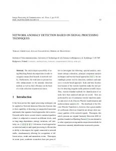
2. Kohonen Self-Organizing Maps In this section, we will review some relative definitions and related works. The dataset can be thought of as a data matrix 𝐷𝑁×𝑀. Each data record corresponds with each row of data matrix and it can be thought of as a mathematical vector which consists of 𝑚 features. Most algorithms need some means of measuring the similarity between two vectors. Euclidean distance formula and cosine formula are often used. In this paper, these two formulas are combined for comparison function. Self-organizing maps have two layers [13]: input layer and output layer. Neurons on the input layer collect the external information to each neuron on the output layer through weight vectors. Input layer has same structure with BP neural network and the number of neurons is equal to the sample dimensions. Output layer is also the compete layer and the arrangement of neurons has diverse forms, such as one-dimension linear array, two-dimension array, and three-dimension grid array. As shown in Figure 1(a), one-dimension SOM is the simplest structure. Neurons on the output layer connect with each other. Figure 1(b) is the structure of two-dimension SOM. This organization form has the image of the cerebral cortex. The learning algorithm of SOM is called Kohonen algorithm which is based on Winner-Take-All algorithm. The
Mobile Information Systems
3
···
···
···
···
···
(a) One-dimension output layer
···
···
(b) Two-dimension output layer
Figure 1: Output layer of SOM.
main difference is the way of adjusting weight vectors and lateral inhibition. For Winner-Take-All algorithm, it only adjusts the winning neuron and other neurons do not change during the update process. However, Kohonen algorithm adjusts not only the winning neuron, but also neurons near by the winner. The impact of winning neuron on other neurons is changed from excitement to inhibition according to the distance between winning neuron and another neuron. Therefore, the learning algorithm adjusts the winning neuron and other neurons around the winning neuron also need to be adjusted by the distance. Self-organizing map is divided into two stages: training stage and testing stage. In the training stage, it chooses the sample randomly from the training dataset and inputs into neural networks. For the specific input pattern, there is a neuron on the output layer that can produce the maximum responsivity and become the wining neuron. But at the beginning of training stage, the location of winning neuron is uncertain. When the input pattern changes, the winning neuron will change. The neurons surrounding with the winning neuron can also produce larger responsivity because of lateral mutual excitatory interactions. Therefore, the weight vectors of winning neuron and neurons nearby will be adjusted towards the input vector and the degree of adjustment is based on the distance between neuron and winning neuron. Self-organizing map trains weight vectors by large amounts of data and finally, neurons on the output layer will be sensitive to corresponding input pattern. When two input patterns are similar, the locations of neurons that represent these patterns are close. After the training of SOM, the specific relation of each neuron on the output layer and input pattern is certain. Now, the trained SOM can be applied as classifier. In the testing stage, the neuron which represents the corresponding pattern will generate the maximum responsivity and classify the input vector automatically when a testing vector is inputted into the network. It is noted that if the pattern of new testing vector does not appear in the training dataset, SOM will mark it as the closest pattern. Researchers have proposed diverse improvements of SOM. In the paper [14], a multiresolution clustering strategy in self-organizing maps is applied to astronomical observations. The authors propose the hierarchical structure of neural networks which consists of different tree-structured SOM networks.
In the paper [15], the authors try to integrate na¨ıve Bayes model with self-organizing map for multidimensional visualization. The proposed method is evaluated by two benchmark datasets and a real-world image processing application which is compared with principal component analysis, selforganizing maps, and generative topographic mapping. The experimental results prove the effectiveness of this method.
3. Improved SOM In this section, we will describe the improved SOM in detail. As the previous analysis, SOM is affected by initial weight vectors. Traditional SOM assigns the value of initial weight vectors randomly and it can result in unstable clustering results just like 𝐾-means. Thus, we improve the way of choosing initial weight vectors and find efficient vectors in training dataset as weight vectors. The comparison function is also improved for measuring the similarity between two vectors more accurately. 3.1. Selecting Initial Weight Vectors. Zhang and Cheng have proposed the optimized method for selecting the initial clustering centers of 𝐾-means clustering algorithm [16]. It uses an adjacent similar degree between data points to calculate similarity density. Then, the data point with the maximum will be utilized as initial clustering centers. Considering the similarity between 𝐾-means and SOM, we apply this optimal method for selecting the initial weight vectors. The details of this method are introduced in the following part. The dataset is denoted by a matrix 𝑋 = {𝑥1 , 𝑥2 , . . . , 𝑥𝑛 } and it is composed of 𝑛 records. 𝑥𝑖 represents the 𝑖th record in the dataset and each record can be denoted as a vector 𝑥𝑖 = {𝑥𝑖1 , 𝑥𝑖2 , . . . , 𝑥𝑖𝑚 } which consists of 𝑚 features. 𝑊𝑗 (𝑗 = 1, 2, . . . , 𝑘) denotes the initial weight vectors. The comparison function for measuring the similarity has diverse methods, such as Euclidean distance formula and cosine distance formula. We use the combination of two distance formulas as the metric of similarity denoted by Sim(𝑥𝑖 , 𝑥𝑗 ) Sim (𝑥𝑖 , 𝑥𝑗 ) = 𝜆𝑑 (𝑥𝑖 , 𝑥𝑗 ) + (1 − 𝜆) cos (𝑥𝑖 , 𝑥𝑗 ) .
(1)
𝑑(𝑥𝑖 , 𝑥𝑗 ) is Euclidean distance formula and cos(𝑥𝑖 , 𝑥𝑗 ) is cosine distance formula. The coefficient 𝜆 is the weighting factor and can be changed from 0 to 1. This coefficient is
4
Mobile Information Systems
adjusted by experimental computation for becoming more suitable in clustering analysis. The less value of Sim(𝑥𝑖 , 𝑥𝑗 ) means the similarity between two vectors 2 𝑑 (𝑥𝑖 , 𝑥𝑗 ) = 𝑥𝑖 − 𝑥𝑗 , 𝑥𝑖 × 𝑥𝑗 cos (𝑥𝑖 , 𝑥𝑗 ) = . 𝑥𝑖 ⋅ 𝑥𝑗
(2)
SimNeighbor(𝑥𝑖 , 𝛼) denotes the similar neighborhood of vector 𝑥𝑖 which is the dataset 𝑋. For other vectors, if the similarity between them and 𝑥𝑖 is less than the threshold, they will be similar neighborhood to 𝑥𝑖 . The method of finding similar neighborhood is as follows: SimNeighbor (𝑥𝑖 , 𝛼) = {𝑥 | 𝛼 ≥ Sim (𝑥, 𝑥𝑖 ) , 0 ≤ 𝛼 ≤ 1, 𝑥 ∈ 𝑋} .
(3)
The value of Sim(𝑥𝑖 , 𝑥𝑗 ) is always greater than (1 − 𝜆). When two vectors are the same, their Euclidean distance is zero and cosine distance comes to the maximum value. The greater the value of Sim(𝑥𝑖 , 𝑥𝑗 ), the lower the degree of similarity. The density of vector 𝑥𝑖 can be calculated according to SimNeighbor(𝑥𝑖 , 𝛼). The calculating formula is as follows: #neighbor(𝑥𝑖 )
Density (𝑥𝑖 ) =
∑𝑗=1
Sim (𝑥𝑖 , neighbor𝑗 (𝑥𝑖 ))
#neighbor (𝑥𝑖 )
. (4)
The symbol #neighbor(𝑥𝑖 ) is the number of SimNeighbor(𝑥𝑖 , 𝛼) and the vector with higher density is more suitable for representing the corresponding pattern of clustering center. The optimal method of selecting initial weight vectors is as follows. Input. The training dataset 𝑋 = {𝑥1 , 𝑥2 , . . . , 𝑥𝑛 }, similarity threshold 𝛼, similar weighting factor 𝜆, initial output layer size. Output. The initial weight vectors. Step 1. Compute the similarity degree between each vector and record in the matrix simMat𝑛×𝑛 . It consists of 𝑛 rows and 𝑛 columns. The value of simMat[𝑖][𝑗] means the similarity degree of 𝑥𝑖 and 𝑥𝑗 . Step 2. Figure out the similar neighborhoods of each vector in dataset 𝑋 according to simMat𝑛×𝑛 and the similarity threshold 𝛼. The similar neighborhood of vector 𝑥𝑖 is stored in Neigh[𝑥𝑖 ]. Step 3. Calculate the density of each vector according to simMat𝑛×𝑛 , the similarity threshold 𝛼, and Neigh[𝑥𝑖 ] that stores the similar neighborhoods. Step 4. Find the vector which has the maximum density and delete it from dataset 𝑋. The similar neighborhood of this vector should also be removed from dataset 𝑋.
Step 5. Calculate the average of the vector which is obtained from Step 4 and its similar neighborhood as one of the initial weight vectors. Step 6. If the size of weight vectors is less than initial output layer size, go to Step 2 and loop the process until it gets enough initial weight vectors. 3.2. The Design of SOM. The input layer of SOM is similar to BP neural network, but the design of output layer is more complicated. It should consider multiple aspects and the preset values may result in different clustering results. The design of output layer needs to consider two aspects. One is the number of neurons and another is the arrangement of these neurons. If the number of neurons is less than the amount of input patterns, SOM cannot recognize all the patterns. But if the number of neurons is much greater, there are some neurons that have not been adjusted, because they are too far from the winning neuron. Therefore, it would be better to give more neurons in advance, in order to map the input patterns onto the appropriate neuron on the output layer. The arrangement of neurons has a lot of choice and it is determined by the practical application. The arrangement of neurons should reflect the physical meaning of the actual problems. For example, in traveling salesman problem, twodimension output layer is more intuitive. For the problem of robot arm control, three-dimension output layer can reflect the spatial characteristics of the arm moment. In our experiences, we utilize two-dimension output layer. In traditional SOM network, the initial weight vector is generated randomly and it can result in worse clustering results. If the initial weight vectors randomly scatter in sample space, they cannot reflect the distribution of samples. Therefore, we choose the average of vectors that are around the winning neuron as the initial weight vector. The selected initial weight vectors can embody the space distribution characteristics of samples. The radius of winning reign should also be taken into consideration. The radius determines whether the neurons should be adjusted and it reduces gradually to zero with the growing number of iterations. In this way, the weight vectors of adjacent neurons are similar but have a little difference. When the winning neurons generate the maximum responsivity, the adjacent neurons will also generate certain responsivity. The calculating formula of radius is as follows: radius (𝑡) = 𝑐 ∗ (1 −
𝑡 ). 𝑡max
(5)
𝑡max is the maximum number of iterations, 𝑡 is the 𝑡th iteration, and 𝑐 is a constant. The learning rate is also selected by experience. 𝜂(𝑡) is the learning rate for the 𝑡th iteration and the value of learning rate can be higher at the beginning of updating weight vectors. But it reduces with the increasing number of iterations. The calculating formula of learning rate is as follows: 𝜂 (𝑡) = exp (−
𝑡 ). 𝑡max
(6)
Mobile Information Systems
5 100
Based on the above analysis, we can obtain the update function of weight vectors as follows:
90 80
+ ℎ𝑐(𝑥),𝑖 (𝑥 (𝑡) − weight𝑖 (𝑡)) , ℎ𝑐(𝑥),𝑖
2 𝑟 − 𝑟 = 𝜂 (𝑡) exp (− 𝑖 𝑐 2 ) . 2 ∗ radius (𝑡)
(7)
𝑟𝑖 is the location of the neuron in the output layer and 𝑟𝑐 is the location of the winning neuron. The distance between two neurons can be calculated by Euclidean distance formula. For example, if the location of 𝑟𝑖 is (0, 0) and 𝑟𝑐 is (1, 1), the distance of them is √2. If 𝑟𝑖 = 𝑟𝑐 , the value of ℎ𝑐(𝑥),𝑖 is 𝜂(𝑡), and it is the learning rate of winning neuron. For other neurons, ℎ𝑐(𝑥),𝑖 will be less than 𝜂(𝑡). To conclude, the steps of updating weight vectors are as follows. Input. The output layer size (𝑁, 𝑀); the number of neurons is 𝑁 ∗ 𝑀; the error threshold diff; training dataset and testing dataset. Output. The analysis result of testing dataset. Step 1. Normalize training dataset and testing dataset. Step 2. Calculate the initial weight vectors and place these neurons to the output layer that can get the location of each neuron. Step 3. Calculate the learning rate, radius, and other coefficients for updating weight vectors by formula (5) and formula (6). Step 4. Choose a vector from training dataset in sequence to update weight vectors by formula (7) while traditional SOM select the training vector randomly. Step 5. If weight𝑖 (𝑡) − weight𝑖+1 (𝑡) < diff, stop training and go to Step 6. Otherwise, go to Step 4. Step 6. Input testing dataset into SOM network and find the winning neuron for each input vector. Input vector will be marked as the pattern of winning neuron.
4. Experience and Analysis In this section, we utilize diverse datasets to evaluate the performance of improved SOM. For applying this improved SOM in anomaly detection, we use KDD CUP 99 dataset for analysis. In the experiments, Algorithm 1 denotes traditional SOM, and Algorithm 2 represents our improved SOM. There are three types of evaluation criteria in our experiments: accuracy rate (AR), precision rate (PR), and recall rate (RR). The calculating formulas are as follows: T, P, F, and N, respectively, stand for true, positive, false, and negative. TP is the number of correctly detected anomaly behaviors and TN is the number of correctly detected normal behaviors. FP is
Accuracy rate
weight𝑖+1 (𝑡) = weight𝑖 (𝑡)
70 60 50 40 30 20 10 0.4
0.5
0.6
0.7
0.8
0.9
1.0
1.1
Similarity threshold
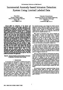
Figure 2: The comparison of different similarity threshold.
the number of falsely labeled anomaly behaviors and FN is the number of falsely labeled normal behaviors. AR =
TP + TN , TP + TN + FP + FN
PR =
TP , TP + FP
RR =
TP . TP + FN
(8)
4.1. The Experiments in Iris Dataset. Firstly, we utilize Iris dataset for evaluating the performance of improved SOM algorithm. In Iris dataset, there are 150 records, and every record consists of 4 features in which the class label is not included. We apply two clustering algorithms to Iris dataset and compare their clustering results. These two algorithms use same parameters: the size of output layer is changing, the maximum number of iterations is 120, diff is set to 0, and similar weighting factor 𝜆 is 0.5. We utilize 80 percent of Iris dataset as training dataset and 20 percent of that as testing dataset. Traditional SOM obtains unstable clustering results, so we repeat it for several times and calculate the average of accuracy rate for comparison. As Table 1 shows, we evaluate improved SOM with different size of output layer. It is obvious that improved SOM can get better clustering results than traditional SOM when they have same size. When the number of neurons is greater than five, the accuracy rate can increase to 100% with the appropriate similarity threshold 𝛼. Then, we analyze the impact of similarity threshold on accuracy rate. The size of output layer is set while the similarity threshold is changing. The results are shown in Figure 2. From Table 1 and Figure 2, we find that accuracy rate changes with the growth value of similarity threshold. It is necessary to find the appropriate similarity threshold for improved SOM. The accuracy rate of improved SOM will be much higher than that of traditional SOM with certain similarity threshold. When the number of neurons is more
6
Mobile Information Systems Table 1: The comparison in Iris dataset.
Size (1, 3) (1, 4) (1, 5) (2, 2) (2, 3) (2, 4) (2, 5) (3, 3) (3, 4) (3, 5) (4, 4) (4, 5) (5, 5)
Algorithm 1 min AR 33.33% 53.33% 43.33% 46.67% 53.33% 53.33% 73.33% 46.67% 73.33% 80.00% 60.00% 63.33% 76.67%
max AR 96.67% 86.67% 96.67% 96.67% 96.67% 93.33% 100.00% 93.33% 100.00% 96.67% 100.00% 100.00% 96.67%
Table 2: The descriptions of datasets. Name Aggregation Compound Flame Jain Path-based Spiral
Samples size
Dimensions
Number of classes
788 399 240 373 300 312
2 2 2 2 2 2
7 6 2 2 3 3
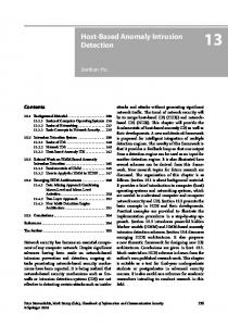
than five, the accuracy rate can be 100% and the number of neurons is same as the number of clusters in another clustering algorithm. 4.2. The Experiments in Universal Datasets. As it shows in the last experiment, the performance of improved SOM is excellent. In order to evaluate the performance of improved SOM on universal datasets, we have selected several datasets from UCI repository. In addition to traditional SOM, we also compare the improved SOM with traditional 𝐾-means and improved 𝐾-means in the paper [17]. The value of 𝐾 is the number of clusters. The characteristics of these datasets are shown in Table 2. To describe the distribution of these datasets, we draw data points in coordinate system as Figure 3 shows. As Figure 3 shows, the distributions of datasets are uneven and two-dimensional. The shapes of these datasets are diverse. We utilize these datasets to evaluate the performances of two clustering algorithms for different shapes. For each dataset, we randomly extract 80 percent records as training dataset and the rest is testing dataset. The results are shown in Table 3. According to the results in Table 3, the performance of improved SOM is better than traditional SOM. When the number of neurons increases to certain value, accuracy rate can become pretty high. But we think the number of neurons should be not more than √𝑛 for the dataset composed of 𝑛
Algorithm 2 Ave Ar 71.00% 72.00% 69.67% 63.33% 74.00% 75.33% 85.67% 76.00% 90.00% 85.00% 83.00% 85.33% 88.67%
Threshold 𝛼 0.90 0.97 0.97 0.97 0.90 0.89 0.88 0.88 0.85 0.69 0.66 0.58 0.51
AR 93.33% 93.33% 100.00% 93.33% 100.00% 100.00% 100.00% 100.00% 100.00% 100.00% 100.00% 100.00% 100.00%
records just the same as 𝐾-means. The clustering result of improved 𝐾-means is better than improved SOM. However, improved 𝐾-means takes more clusters than improved SOM, which need high time and space overhead. For spiral dataset, its shape is complex and improved SOM cannot get superior results when the size of output layer is (4, 4). However, the accuracy rate will increase to 100% when the size is set to (7, 9). 4.3. The Experiments in KDD Cup99 Dataset. In order to evaluate the performance of improved SOM applied for anomaly detection, we utilize KDD Cup99 dataset to compare two clustering algorithms. KDD Cup99 dataset is extracted from real network environment and there are about 5 million records in KDD Cup99 dataset. Each record consists of 42 features which include the label of normal and attack type. We extract 2100 records from KDD Cup99 dataset which is composed of 2000 normal records and 100 attack records. The attack records consist of four types of attack. The labels of attack records are back, teardrop, smurf, and neptune. Before the experiments, we delete symbolical features, and numerical features are left. The clustering results are shown in Table 4. As Table 4 shows, improved SOM can obtain better performance comparing with traditional SOM in the same size of output layer. There are too few attack records for traditional SOM to detect them. The number of neurons determines precision rate and recall rate of traditional SOM. However, improved SOM can get higher precision rate and recall rate with less number of neurons. The clustering results of improved SOM are affected by the shape of output layer and similarity threshold. The increasing of similarity threshold can improve recall rate, but when the size of output layer comes to (8, 8), precision rate starts to decrease if similarity threshold is too large. The similarity threshold has particular influence on the clustering results, because it is used for selecting initial weight vectors. To analyze the impact of similarity threshold in KDD Cup99 dataset, we change the value of similarity threshold
Size
(4, 6) (4, 4) (3, 3) (2, 4) (3, 5) (4, 4)
Dataset
Aggregation Compound Flame Jain Path-based Spiral
max AR 98.73% 87.50% 100.00% 97.33% 93.33% 82.54%
Algorithm 1 min AR 89.24% 78.75% 85.42% 89.33% 71.67% 30.15% Ave AR 93.48% 83.50% 92.08% 92.13% 83.33% 56.03%
Algorithm 2 Threshold AR 0.771 99.37% 0.72 93.75% 0.75 100.00% 0.89 100.00% 0.51 90.00% 0.51 66.67%
Table 3: The results on universal datasets. Traditional 𝐾-means 𝐾 Ave AR 40 99.56% 49 97.64% 55 98.92% 29 99.95% 50 99.00% 27 84.36%
Improved 𝐾-means 𝐾 AR 40 99.62% 49 99.00% 55 100.00% 29 100.00% 50 100.00% 27 100.00%
Mobile Information Systems 7
8
Mobile Information Systems Aggregation
30
20
20
24 22
15
15 10
20 18
10
5
16 0
5
10
20
15
25
30
35
40
Jain
30
20 15 10 5 0
5
10
15
20
25
5
5
10
15
30
35
40
45
20
25
30
35
40
45
Path-based
35
25
0
Flame
28 26
25
0
Compound
25
14
30
25
25
20
20
15
15
10
10
5
5 0
5
10
15
20
2
4
8
6
25
30
35
0
10
12
14
16
30
35
Spiral
35
30
0
0
0
5
10
15
20
25
Figure 3: The distribution of datasets. Table 4: The results in KDD Cup99 dataset. Size (5, 5) (6, 6) (7, 7) (8, 8) (9, 9)
Algorithm 1 Ave RR 8.00% 8.50% 14.00% 17.50% 23.50%
Ave PR 40.00% 40.00% 70.00% 66.67% 90.00%
Table 5: The comparison of different similarity threshold in KDD Cup99. Similarity threshold 1.0 1.5 2.0 2.5 3.0 3.5
Improved SOM Recall rate Precision rate 80.00% 88.89% 85.00% 85.00% 60.00% 100.00% 100.00% 95.24% 75.00% 93.75% 75.00% 93.75%
while the size of output layer is constant. The results are shown in Table 5. From Table 5 and Figure 2, we find that recall rate and precision rate fluctuate with the increasing of similarity threshold. It is necessary for improved SOM to find the appropriate value of similarity threshold. In this way, improved SOM can get better results in the case of less neurons.
Threshold 3.0 3.0 2.5 2.0 1.5
Algorithm 2 RR 75.00% 75.00% 100.00% 100.00% 100.00%
PR 93.75% 93.75% 95.24% 76.92% 100.00%
5. Conclusion Traditional SOM is affected by initial weight vectors and it generates unstable clustering results. To overcome these shortcomings, this paper proposes an improved SOM clustering algorithm and compares it with traditional one. We utilize the optimal method to select more suitable initial weight vectors. In this way, SOM can obtain more appropriate initial weight vectors that will generate more stable and accurate results. To analyze this improved clustering algorithm, we utilize diverse datasets to evaluate the performances of improved SOM. As the experimental results show, improved SOM can get higher accurate rates for each dataset. And the performance of improved SOM on KDD Cup99 is also better than traditional SOM. However, there are some aspects that can be improved in our algorithm. Firstly, the process of finding initial weight vectors is time-consuming and it makes improved SOM spends more time than traditional one. Secondly, the fuzzy theory [18] can be introduced to improve the ability applied in
Mobile Information Systems practical environment. Last, the size of output layer is determined by experience and it can be modified to be decided automatically.
Competing Interests The authors declare that they do not have any conflict of interests related to this work.
Acknowledgments This work was funded by the National Natural Science Foundation of China (61373134). It was also supported by the Priority Academic Program Development of Jiangsu Higher Education Institutions (PAPD), Jiangsu Key Laboratory of Meteorological Observation and Information Processing (KDXS1105), and Jiangsu Collaborative Innovation Center on Atmospheric Environment and Equipment Technology (CICAEET).
References [1] A.-D. Schmidt, F. Peters, F. Lamour, C. Scheel, S. A. C ¸ amtepe, and S¸. Albayrak, “Monitoring smartphones for anomaly detection,” Mobile Networks and Applications, vol. 14, no. 1, pp. 92– 106, 2009. [2] M. Anagnostopoulos, G. Kambourakis, and S. Gritzalis, “New facets of mobile botnet: architecture and evaluation,” International Journal of Information Security, vol. 15, no. 5, pp. 455–473, 2015. [3] A. Pawling, N. V. Chawla, and G. Madey, “Anomaly detection in a mobile communication network,” Computational and Mathematical Organization Theory, vol. 13, no. 4, pp. 407–422, 2007. [4] Y. Zhou and X. Jiang, “Dissecting Android malware: characterization and evolution,” in Proceedings of the 33rd IEEE Symposium on Security and Privacy, pp. 95–109, San Francisco, Calif, USA, May 2012. [5] C. Yin, L. Ma, and L. Feng, “A feature selection method for improved clonal algorithm towards intrusion detection,” International Journal of Pattern Recognition and Artificial Intelligence, vol. 30, no. 5, Article ID 1659013, 14 pages, 2016. [6] B. Gu, V. S. Sheng, K. Y. Tay, W. Romano, and S. Li, “Incremental support vector learning for ordinal regression,” IEEE Transactions on Neural Networks and Learning Systems, vol. 26, no. 7, pp. 1403–1416, 2015. [7] B. Gu, V. S. Sheng, Z. Wang, D. Ho, S. Osman, and S. Li, “Incremental learning for ]-support vector regression,” Neural Networks, vol. 67, pp. 140–150, 2015. [8] A. Forestiero, “Self-organizing anomaly detection in data streams,” Information Sciences, vol. 373, pp. 321–336, 2016. [9] C. Yin, L. Feng, and L. Ma, “An improved Hoeffding-ID datastream classification algorithm,” Journal of Supercomputing, vol. 72, no. 7, pp. 2670–2681, 2016. [10] C. Yin, S. Zhang, J. Xi, and J. Wang, “An improved anonymity model for big data security based on clustering algorithm,” Concurrency and Computation: Practice and Experience, 2016. [11] A. Hadian and S. Shahrivari, “High performance parallel k-means clustering for disk-resident datasets on multi-core CPUs,” Journal of Supercomputing, vol. 69, no. 2, pp. 845–863, 2014.
9 [12] T. Kohonen, Self-organizing maps, vol. 30 of Springer Series in Information Sciences, Springer, Berlin, Germany, Second edition, 1997. [13] T. Kohonen, “Essentials of the self-organizing map,” Neural Networks the Official Journal of the International Neural Network Society, vol. 37, no. 1, pp. 52–65, 2012. [14] D. Ord´on˜ ez, C. Dafonte, B. Arcay, and M. Manteiga, “HSC: a multi-resolution clustering strategy in Self-Organizing Maps applied to astronomical observations,” Applied Soft Computing Journal, vol. 12, no. 1, pp. 204–215, 2012. [15] G. A. Ruz and D. T. Pham, “NBSOM: the naive Bayes self-organizing map,” Neural Computing and Applications, vol. 21, no. 6, pp. 1319–1330, 2012. [16] Y. Zhang and E. Cheng, “An optimized method for selection of the initial centers of K-means clustering,” Lecture Notes in Computer Science (including subseries Lecture Notes in Artificial Intelligence and Lecture Notes in Bioinformatics), vol. 8032, pp. 149–156, 2013. [17] C. Yin and S. Zhang, “Parallel implementing improved k-means applied for image retrieval and anomaly detection,” Multimedia Tools and Applications, pp. 1–17, 2016. [18] J. C. Bezdek, R. Ehrlich, and W. Full, “FCM: the fuzzy c-means clustering algorithm,” Computers and Geosciences, vol. 10, no. 23, pp. 191–203, 1984.
Journal of
Advances in
Industrial Engineering
Multimedia
Hindawi Publishing Corporation http://www.hindawi.com
The Scientific World Journal Volume 2014
Hindawi Publishing Corporation http://www.hindawi.com
Volume 2014
Applied Computational Intelligence and Soft Computing
International Journal of
Distributed Sensor Networks Hindawi Publishing Corporation http://www.hindawi.com
Volume 2014
Hindawi Publishing Corporation http://www.hindawi.com
Volume 2014
Hindawi Publishing Corporation http://www.hindawi.com
Volume 2014
Advances in
Fuzzy Systems Modelling & Simulation in Engineering Hindawi Publishing Corporation http://www.hindawi.com
Hindawi Publishing Corporation http://www.hindawi.com
Volume 2014
Volume 2014
Submit your manuscripts at https://www.hindawi.com
Journal of
Computer Networks and Communications
Advances in
Artificial Intelligence Hindawi Publishing Corporation http://www.hindawi.com
Hindawi Publishing Corporation http://www.hindawi.com
Volume 2014
International Journal of
Biomedical Imaging
Volume 2014
Advances in
Artificial Neural Systems
International Journal of
Computer Engineering
Computer Games Technology
Hindawi Publishing Corporation http://www.hindawi.com
Hindawi Publishing Corporation http://www.hindawi.com
Advances in
Volume 2014
Advances in
Software Engineering Volume 2014
Hindawi Publishing Corporation http://www.hindawi.com
Volume 2014
Hindawi Publishing Corporation http://www.hindawi.com
Volume 2014
Hindawi Publishing Corporation http://www.hindawi.com
Volume 2014
International Journal of
Reconfigurable Computing
Robotics Hindawi Publishing Corporation http://www.hindawi.com
Computational Intelligence and Neuroscience
Advances in
Human-Computer Interaction
Journal of
Volume 2014
Hindawi Publishing Corporation http://www.hindawi.com
Volume 2014
Hindawi Publishing Corporation http://www.hindawi.com
Journal of
Electrical and Computer Engineering Volume 2014
Hindawi Publishing Corporation http://www.hindawi.com
Volume 2014
Hindawi Publishing Corporation http://www.hindawi.com
Volume 2014