Abstract. In this paper, we have analyzed the dynamics of a mag- netic guiding system and derived its analytical model with full DOFs (degrees-of-fieedom).
Proceedings of the American Control Conference
San Diego, California June 1999
Modeling and Controller Design of a MAGLEV Guiding System for Application in Precision Positioning Mei-Yung Chen’, Ming-Jyh Wang’, Li-Chen FU’?~ I . Department of Electrical Engineering, National Taiwan University, Taipei, Taiwan, Republic of China. 2. Department of Computer Science and Information Engineering, National Taiwan University, Taipei, Taiwan, Republic of China.
Abstract In this paper, we have analyzed the dynamics of a magnetic guiding system and derived its analytical model with full DOFs (degrees-of-fieedom). Then, an adaptive controller which deals with unknown parameters is proposed here to regulate the five DOFs in this system. The guiding system including sensors and drivers systems is actually implemented. From the experimental results, satisfactory performance including stifhess and resolution have been achieved. This validates, the design of system hardware and demonstrates feasibility of the developed controller. Keywords: Maglev, Hybrid magnet, Adaptive control, Precision positioning
1. Introduction Recently, magnetic levitation is considered as one of the most suitable ways to achieve the high precision transportation. By Hollis et al.[l][2], it creates a stable state without any mechanical contact when the gravitational force is solely counterbalanced by magnetic forces. Of course, such contact-fiee levitation has to be enforced for all DOFs of the rigid body. Often, a distinction is made between magnetic suspension and magnetic levitation. The former refers to systems based on attractive magnetic forces whereas the latter based on repulsive ones. However, this restricted sense of the two terms does not cover all types of contact-free magnetic support. Therefore, it is the current trend to use the term ‘levitation’ in a more general sense, and to abbreviate “magnetic levitation” as ‘maglev’ in short. Previous work in maglev system spans many fields. A large volume of literature has been published. Some well known fields include maglev transportation[3][4], wind tunnel levitation[S], magnetic bearings[6], and antivibration tables[7]. Here, however, we will only investigate
0-7803-4990-6199 $10.000 1999 AACC
the maglev techniques for the field of short-range travel with precision positioning and then design and implement a prototype maglev system to verify its high performance. In this paper, a prototype maglev guiding system is built, which takes concept similar to those in[8],[9], and a complete analytical model, including five degrees of fieedom is derived, i.e., without considering the degree for large-range actuation. Furthermore, an adaptive controller which achieves the guiding goals is developed. Experimental results are obtained to demonstrate the feasibility of this guiding system. The organization of this paper is as follows. In section 2 describes the design aspects of the hereby implemented prototype system, and derives detailed mathematic model. In section 3, a adaptive controller for the prototype maglev system is developed. Section 4 presents extensive experimental results to demonstrate the effectiveness of the system design and its controller. Some discussion is also made is section 4. Finally, conclusions are drawn in section 5.
2.System Description and Modeling In this section, the mechanical design of a maglev guiding system will be introduced. Its analytical model of full DOFs will be derived and analyzed.
2-1.Maglev Guiding System In a stepper, one always find a linear slide to support and to guide the carrier. The system proposed here is featured in an active .control to provide a contactless linear slide as mentioned,which however is different from the magnetic bearing of rotating machine. For detailed design of the system, one can refer to [ 9 ] . In this section, only brief description will be given. The features of this maglev guiding system include: (1) repulsive levitation, (2) hybrid magnets, (3) passive carrier and active track, (4) oblong coil concept and (5) four-track
3072
D are I,, z, I, and I D , respectively. Let I,, and I,, represent the moments of inertia with respect to the axes parallel to the Y axis at the points A and C. After a series of simplification and the dropping the of 6 sign, we finally obtain:
design. The front view of overall system is shown as Fig. 1. stabilizingcoils
/
levitationcoils I \
\
& = 4KPxLX+ 2K,(Il +I,)
[,e= 4a’Km@ + 2aK,(Il I
I
Track I
Track
n
I
I
&=4KFzLZ+2Km(411+bJ2)b+K,z(IA+ I , + I c + I o ) I,? = 21 (- 1 + -)KNLX 1 + 2aIy(- 1 + -)KNL8 1 + 2IY&
I
I
Trackm
Trackm
Figure 1: Front view of overall system
[”U
4 0
‘A0
+2[(4’ +b:)Km
2-2.Analytical Model
In carrier design, we have chosen the material to ensure the rigidity of the carrier. To understand the dynamics of a rigid body, it is necessary to know how to describe an arbitrary orientation of a rigid body in space. Here, we adopt zy-x Eulerian angle orientational representation. Let the xyz coordinate system be fixed on the carrier and the XYZ coordinate system be fixed on the track, shown as Fig.2.
ryt
‘AW.
(3)
- I,)
‘CU
+ A)K,,.J C ‘O
‘A0
+2(b,’II+ $ I 2 ) K m ~ + Ik I Y ( 1 - ~ ) K ~ ‘A0
‘CU
+2KILL[4(IA -IBl+b2(’C - I D ) ] 1,@=2a(411 - h J , ) K ~ + 4 a z K m ~ + a K , ( I A+ I , - I c - I o )
where K,. are destabilizing force constants, K,. are constant relating the stabilizing force and the driving current. carrier
Figure 3: Positions of levitation magnets
CarrierCwmidate
rlr
Figure 2: Eulerian Angles
3.Controller Design
Consider the carrier to be represented by a uniform box shaped object with the center of mass coincident with the center of geometry. Assume small displacements in rotation and translation and neglect the higher-order terms. Based on Newton-Euler method, we can obtain:
From the modeling process described in the previous section, several assumptions have been made which inevitably will cause some modeling errors. Therefore, the controller to be developed should be robust enough to tolerate these system uncertainties and unmodeling dynamics. Here, we prefer to choose the adaptive control as a solving tool.
F,=&
F,=mZ
(1)
where F, F, are the resultant forces acting on the carrier along the X-axis and Z-axis and m is the mass of the carrier, and w,@,e are the three Eulerian angles of the rigid body. Moreover, T, = I,? T, = 1,4 T, = 1,e (2)
3-1.Plant Model In order to obtain a compact controller, we redefine the control inputs as (4)
where T, ,T, and T, are the external torques, I,, 1, and 1, are the principle moments of inertia. Substituting the positions of the levitation magnet as shown in Fig. 3 into force equations and torque equations in Eqs (1)(2), we can then get the forces and torques exerted on each levitation magnet. Next, substitute these force and torque equation into dynamics of carrier, then one can obtain the model of this maglev guiding system. Before that, define the control current in the inner stabilizer as[,, whereas in the outer stabilizer as I,. Control currents in levitators corresponding the levitation magnets A, B, C and
where 1, = IB and the transformation matrices in Eq. (4) and Eq. ( 5 ) are invertible. Also, to facilitate the design of a singularity-fiee adaptive controller, we rewrite the plant model discussed by Eq. (3) as:
b , , X = a , , X - U, + V , b,,B = a,,8 - U, + v 2
3073
b3,Z = a& + a3,u14+ a32u24+ u3 + v3 b-$=a,,X +a,,8+a,,u,Z+a,,u2Z
4 ,ji =a, ,X+VI - 6,(@ +q x )-;i,x-Cl (13) =-41(4X+qx>+qJ+&~4~ +F where GI =a,,-GI, 4, =4, -&, =v, -Cl and 6 =,$x+qX.
(8) (9)
+a44~+a46161~+a47u2~+a48Ul~+a49u2~+u4
+v4
(10)
bs5@ = a5lul4 + QSZU24 + a55w + us + vs
Define
whereh, > O for i=1-5, U,, > 0 for i=1-2, a,, < 0 for i=3-5. Additionally,v, ,Vi=1-5 do not appear in Eq. (3), but they are modeled here in order to cancel the sensor calibration error. These errors are due to the mismatches between the actual neutral points (tracks) and the chosen neutral points (sensors) as shown in Fig. 4, and can be further reduced by calibration of the precision equipment. In Eqs. (6) and (7),Xand@ are decoupled fiom the other states, and can be controlled byu, and u2 properly. The signals X,8,U, and u2 in Eqs. (8) to (1 0) are measurable, and if the controllers for Xand 0 can assure their boundedness, they can be used as known and bounded terms for the controller design of 2, 4 and w . Rewrite the Eqs. (8) to (10) as
DBE= -D,E + U + g ( X ,Q,Z,4, v,U, y ) + v
[
a4,u2Z+ w a51.14
&,
3074
B. Vertical Control
t', = @D,S + ~&G;BJ
DA = - G A S E T ,where G , = diag(gal,gat,ga3)
where
fiB = G$NT, where G , = diUg(gb,,gb,,g,,) C = G,S, =g31s3'l$9~32
=g32s3uZ$?~41
=g41s4x3'42.
&3
= g 4 3 '4
= g4.5'4
= g 4 6 '4
I'
2 '
'?5
a 4 8 =g48s4uly/,rfr4g
I '
Y'
4;,
=g49s4u2~,'51
1'
=g51s5'l$Y
= g47'4
gi;z32g?2
,3+ ,4' l ; ,g
+ gi:z48z48
=g4ZS4'Y 4 7 L?,'
'
4 =g~~'3IS,l
where G , = diag(g,,,gV2,gv3)
;3l
+ ~ % ~ ; f +YG;~V+Q) i~) (27)
'2
$3
' 5 2 =g52'5'2$
+
gii'49'49
-k
s,;''41a"?l
+ g~~'42'$7
i- g2k6!,.5
'
g;:'51z51
+ g 3 4 7 3 ,
+ g;:'52'52
- f i A+~i j , +~ g + v ) + t r ( ~ ~ G , ' ~ B ) + r r ( % j ; G , ' ?G;%++q fiA)+
= s'(-D,A,s
(22)
= -S'D,A,S
3-4.Stability Analysis
In order to prove the stability of the closed-loop h c tion Eq. (15), we can choose a Lyapunov function candidate? as:
gi;'4+45
Substituting Eq. (20) and adaptive laws in Eq. (22) into Eq. (27), we can obtain:
where g, > 0 Vi,j .
Here, we will prove that all the error states are asymptotically stable. A. Lateral Control
+
5
(28)
o
whereD ~ are A ~diagonal matrix with positive diagonal terms. From Eqs. (26) and (28), it shows that Vz is a suitable Lyapunov function, and, by Lyapunov stability criteria, we conclude that S, bA, G,, 7 and parameters exist in q are all bounded, s and in turn S E L , by referring back to Eq. (20). Thus, by using Barbalat's Lemma, we finally have that s asymptotically stable. So we can further y/ and ci/ are asymptoticallystable. conclude z, 2, 4,
4,
-
where y o > 0, forj = 1 3 .
4.Experimental Results
Its time derivative can be evaluated as:
Substituting Eq. (1 5) and adaptive laws in Eq. (2 1) into Eq. (24), we can obtain:
Figure 5 is the system block diagram which illustrates the overview of the operation flow. Figures 6 shows the photographs of the physical set-up. This sensor system, which is divided into lateral and vertical sensor subsystems, respectively, will provide two translational and three rotational disolacement data for the controller. For sensor detailed discussions, the readers should refer them to [9].
=+g50 From Eqs. (23) and (25), it shows that j( is a suitable Lyapunov function, and, by Lyapunov stability criteria, we conclude that s, ,&, gl1and TI are all bounded, si E L, and in turn SI E L, by referring back to Eq. (15). Thus, by using Barbalat's Lemma[l2], we finally have that s1 asymptotically stable. From the definition S, = k1 + Alxl,A, > 0,we can M e r concludeXI are asymptoticallystable. B. Vertical control To prove the stability of the close-loop function Eq. (20), we can choose a Lyapunov function candidate Vz as: 1 V2 = -(STD,S+ rr(D$: 2
where q = g;:a;: + g;;.":,
DE) +r