Modeling, Evaluation, and Testing of Paradyn ... - Semantic Scholar

Modeling, Evaluation, and Testing of Paradyn Instrumentation System* Abdul Waheed and Diane T. Rover * Department of Electrical Engineering Michigan State University E-mail: {waheed,rover}@egr.msu.edu

Jeffrey K. Hollingsworth Department of Computer Science University of Maryland E-mail: [email protected]

Abstract This paper presents a case study of modeling, evaluating, and testing the data collection services (called an instrumentation system) of the Paradyn parallel performance measurement tool. The overall objective of the study is to use modeling- and simulation-based evaluation and provide feedback to the tool developers. An early feedback regarding instrumentation system overhead and performance helps the developers choose appropriate system configurations and task scheduling policies. We develop a resource occupancy model for the Paradyn instrumentation system (IS) and parameterize it for an IBM SP-2 platform. This model is parameterized with a measurement-based workload characterization and subsequently used to answer several “what if” questions regarding two policies to schedule instrumentation system tasks: collect-and-forward (CF) and batch-andforward (BF) policies for three types of architectures: network of workstations (NOW), shared memory multiprocessors (SMP), and massively parallel processing (MPP) systems. In addition to comparing the two scheduling policies, the study also investigates two options for forwarding the instrumentation data: direct and binary tree forwarding for the MPP system. Simulation results indicate that the BF policy can significantly reduce the overheads. Based on this feedback, the BF policy was implemented in the Paradyn IS as an option to manage the data collection. Measurement-based testing results obtained from this enhanced version of the Paradyn IS are reported in this paper and indicate more than 60% reduction in the direct IS overheads when the BF policy is used.

1

Introduction

Application-level software instrumentation systems (ISs) collect runtime information from parallel and distributed systems. This information is collected to serve various purposes, for example, evaluation of program execution on high performance computing and communication (HPCC) systems [23], monitoring of distributed real-time control systems [3,10], resource

* This

work was supported in part by DARPA contract No. DABT 63-95-C-0072 and National Science Foundation grant ASC-9624149. 1

management for real-time systems [18], and administration of enterprise-wide transaction processing systems [1]. In each of these application domains, different demands may be placed on the IS and it should be designed accordingly. In this paper, we present a case study on IS design; we apply a structured development approach to the instrumentation system of the Paradyn parallel performance measurement tool [20]. This structured approach is based on modeling and simulating the IS to answer several “what-if” questions regarding possible configurations and scheduling policies to collect and manage runtime data [28]. The Paradyn IS is enhanced based on the initial feedback provided by the modeling and simulation process. Measurement-based testing validates the simulation-based results and shows more than 60% reduction in the data collection overheads for two applications from the NAS benchmark suite executed on an IBM SP-2 system. Using principal component analysis on these measurements, we also show that the reduction of overheads is not affected by the choice of an application program. A rigorous system development process typically involves evaluation and testing prior to system production or usage. In IS development, formal evaluation of options for configuring modules, scheduling tasks, and instituting policies should occur early. Testing then validates these evaluation results and qualifies other functional and non-functional properties. Finally, the IS is deployed on real applications. Evaluation and testing require a model for the IS and adequate characterization of the workload that drives the model. The model can be evaluated analytically or through simulations to provide feedback to IS developers. The model and workload characterization also facilitate testing by highlighting performance-critical aspects. In this paper, we focus on evaluation and testing of the Paradyn IS. One may ask if such rigor is needed in IS development. The IS represents enabling technology of growing importance for effectively using parallel/distributed systems. The IS often supports tools accessed by end-users; the user typically sees the tool and not the IS. Consequently, tools are scrutinized, and the IS and its overheads receive little attention. Users may be unaware of the impact of the IS. Unfortunately, the IS can perturb the behavior of the application [17], degrading the performance of an instrumented application program from 10% to more than 50% according to various measurement-based studies [8,19]. Perturbation can result from contention for system resources among application and instrumentation processes. With increasing sophistication of system software technologies (such as multithreading), an IS process is expected to manage and 2

regulate its use of shared system resources [24]. Toward this end, tool developers have implemented adaptive IS management approaches; for instance, Paradyn’s dynamic cost model [12] and Pablo’s user-specified (static) tracing levels [23]. With these advancements come increased complexity and more design decisions. Dealing with these design decisions is the topic of this paper. A Resource OCCupancy (ROCC) model for the Paradyn IS is developed and parameterized in Section 2. We simulate the ROCC model to answer a number of interesting “what-if” questions regarding the performance of the IS in Section 4. Modifications to the Paradyn IS design are tested in Section 5 to assess their impact on IS performance. We conclude with a discussion of the contributions of this work to the area of parallel tool development.

2

A Model for Paradyn IS

In this section, we introduce Paradyn and present a model for its IS. Paradyn is a tool for measuring the performance of large-scale parallel programs. Its goal is to provide detailed, flexible performance information without incurring the space and time overheads typically associated with trace-based tools [20]. The Paradyn parallel performance measurement tool runs on TMC CM-5, IBM SP-2, and clusters of Unix workstations. We have modeled the Paradyn IS for an IBM SP-2 system. The tool consists of the main Paradyn process, one or more Paradyn daemons, and external visualization processes. The main Paradyn process is the central part of the tool, which is implemented as a multithreaded process. It includes the Performance Consultant, Data Manager, and User Interface Manager. The Data Manager handles requests from other threads for data collection, delivers performance data from the Paradyn daemon(s), and distributes performance metrics. The User Interface Manager provides visual access to the system’s main controls and performance data. The Performance Consultant controls the automated search for performance problems, requesting and receiving performance data from the Data Manager. Paradyn daemons are responsible for inserting the requested instrumentation into the executing processes being monitored. The Paradyn IS supports the W3 search algorithm implemented by the Performance Consultant for on-the-fly bottleneck searching by periodically providing

3

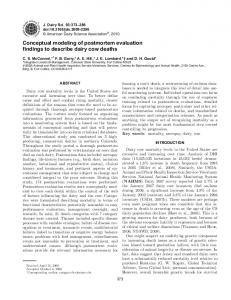
instrumentation data to the main Paradyn process [11]. Required instrumentation data samples are collected from the application processes executing on each node of the system. These samples are collected by the local Paradyn daemon (Pd) through Unix pipes, which forwards them to the main process. Figure 1 represents the overall structure of the Paradyn IS. In the figure, pji for j =0,1,..., n-1 denote the application processes that are instrumented by a local Paradyn daemon at node i, where the number of application processes n at a given node may differ from another node.

main process

Main Paradyn process

Host workstation Paradyn daemons

Application processes

Pd

p0 0

Pd

... pn-10

pn-1P-1

p0P-1

Node 0

Node P-1

Figure 1. An overview of the Paradyn IS [20].

2.1 Queuing Network Model The Paradyn IS can be represented by a queuing network model, as shown in Figure 2. It consists of several sets of identical subnetworks representing a local Paradyn daemon and application processes. We assume that the subnetworks at every node in the concurrent system show identical behavior in terms of sharing local resource during the execution of an SPMD program. This assumption helps maintain the focus on two levels of detail for this study: local details of resource sharing at every node and global details of overall system behavior, performance, and interactions among the system nodes. At a local level of detail, the focus of this study is resource sharing among processes at a node by considering only one subnetwork at a given node and applying the ROCC model, introduced in the next section, for evaluation. At the global level of detail, the subnetworks interact with one another using a shared network (in case of NOW), a bus (in case of SMP), or a high-performance, dedicated network (in case of MPP). Figure 2 highlights the performance data collection and forwarding activities of a Paradyn daemon on a node. These IS activities are central to Paradyn’s support for on-line analysis of performance bottlenecks in long-running application programs. However, they may adversely

4

p0 i

Data collection by a Pd

Pd0

...

p1 i

...

Pdi

pn-1i

...

PdP-1

Data forwarding by a Pd

Local application processes (n) on node i Instrumentation data buffers provided by the kernel (Unix pipes)

Local Paradyn daemons (P), one per node Network delays are represented by the arrivals to a single server buffer to allow random sequence of arrivals from different Pds

Main process


Figure 2. A model for the Paradyn instrumentation system.

affect application program performance, since they compete with application processes for shared system resources. Objectives of our modeling include evaluating IS overheads due to resource sharing, identifying any IS-induced performance bottlenecks, and determining desirable operating conditions for the IS. Scheduling Policies for Data Forwarding. Two possible options for a Paradyn daemon to schedule

data collection and data forwarding at a node are collect-and-forward (CF) and batch-andforward (BF). As illustrated in Figure 3, under the CF scheduling policy, the Paradyn daemon collects a sample from an instrumented application process and immediately forwards it to the main process. Under the BF policy, the Pd collects a sample from the application process and stores it in a buffer until a batch of an appropriate number of samples is accumulated, which is then forwarded to the main Paradyn process. To main Paradyn

To main Paradyn Paradynd Processes Buffer size = 1

Paradynd Processes

(a) CF policy

Buffer size > 1 (b) BF policy

Figure 3. Two policies for scheduling data collection and forwarding: (a) collect-and-forward (CF) policy and (b) batch-and-forward (BF) policies.

5

IS Configurations for Data Forwarding. In case of using Paradyn IS on an MPP system, we

consider two options for forwarding the instrumentation data from the Paradyn daemon to the main Paradyn process: direct forwarding and binary tree forwarding. Under the configuration for direct forwarding, a Paradyn daemon directly forwards one or multiple samples (under the CF and BF policies, respectively) to the main Paradyn process. Under the binary tree forwarding scheme, the system nodes are logically arranged as a binary tree and every Paradyn daemon running on a non-leaf node receives, processes, and merges the samples or batches from Paradyn daemon running on its two children nodes. Figure 4 illustrates the two configurations. Paradyn

Pd

Pd

Pd

Paradyn Pd

Pd

Pd

Pd

(a) Direct forwarding

Pd Pd

(b) Binary tree forwarding

Figure 4. Two configurations for data forwarding for MPP implementation of Paradyn IS: (a) direct and (b) binary tree forwarding.

Metrics. We use two sets of performance metrics corresponding to global and local levels of detail.

Two performance metrics are of interest for the global levels of detail of this study: average direct overhead due to IS modules and monitoring latency of data forwarding. Average direct overhead represents the occupancy time of a shared system resource by the IS modules, which is averaged over all the system nodes. A lower value of the direct overhead is desirable. Monitoring latency has been defined as the amount of time between the generation of instrumentation data and its receipt at a logically central collection facility (in our case, the main Paradyn process) [8]. At a local level of detail, two metrics are comparable to metrics at the global level: direct overhead of data collection and throughput of data forwarding. Interpretation of the direct overhead is same as in the case of global level without averaging over all the nodes. It quantifies the contention between application and IS processes for the shared resources on a particular node of the system. Throughput of a Paradyn daemon impacts the main Paradyn process, since a steady flow of data samples from individual system nodes is needed to allow the bottleneck searching algorithm to work properly. Throughput of data forwarding by a Paradyn daemon is directly related to the monitoring latency. A higher throughput means lower monitoring latency and vice versa. Thus, a higher value of throughput is desirable.

6

Simulation-based experiments presented in Section 4 calculate these metrics to help answer a number of “what-if” questions. Metrics for global level of detail are calculated for the entire system while those for the local level are calculated at an arbitrarily selected node. 2.2 Resource Occupancy Model This subsection introduces the Resource OCCupancy (ROCC) model and its application to isolating the overheads due to non-deterministic sharing of resources between the Paradyn IS and application processes [29]. The ROCC model, founded on well-known computer system modeling techniques, consists of three components: system resources, requests, and management policies. Resources are shared among (instrumented) application processes, other user and system processes, and IS processes; for example, CPU, network, and I/O devices. Requests are demands from application, other user, and IS processes to occupy the system resources during the execution of an instrumented application program. A request to occupy a resource specifies the amount of time needed for a single computation, communication, or I/O step of a process. IS management involves scheduling of system resources to perform data collection and forwarding activities. Figure 5 depicts the ROCC model with local and global levels of detail. It includes two types of resources of interest for the Paradyn IS, CPUs and network, being shared by three types of processes on every node: application, IS, and other user processes. Due to the interactions among different types of processes at the same node and IS processes at multiple nodes, it is impractical to solve the ROCC model analytically. Therefore, simulation is a natural choice. The execution of the ROCC model for the Paradyn IS relies on a workload characterization of the target system, which in turn, relies on measurement-based information from the specific system [5,13]. 2.3 Workload Characterization The workload characterization for this study has two objectives: (1) to determine representative behavior of each process of interest (i.e., application, IS, and other user/system processes) at a system node (see section 2.3.1); and (2) to fit appropriate theoretical probability distributions to the lengths of resource occupancy requests from each of these processes (see section 2.3.2). The resulting workload model is both practical and realistic.

7

Triggering of subsequent request from the corresponding process Instrumented application processes

Time out Serviced CPU requests from the other processes

Instrumentation system processes

Other user/system processes

CPU Requests

Processes running at a particular system node that generate requests for occupying the system resources

...

CPU

...

Network

Network Requests

(a) ROCC model for a particular system node Instrumentation data forwarding (in case of binary tree configuration)

ROCC model for CPU occupancy at a node

Node processes


Node processes


...

Node processes

Network

...

...

(b) ROCC model for the entire system Figure 5. The resource occupancy model for the Paradyn IS with (a) local and (b) global levels of detail.

2.3.1 Process Model

We consider the states of an instrumented process running on a node, as illustrated by Figure 6, which is an extension of the Unix process behavior model. After the process has been admitted, it can be in one of the following states: Ready, Running, Communication, or Blocked (for I/O). The process can be preempted by the operating system to ensure fair scheduling of multiple processes sharing the CPU. After specified intervals of time (in case of sampling) or after occurrence of an event of interest (in case of tracing), such as spawning a new process, instrumentation data are

8

collected from the process and forwarded over the network to the main Paradyn process via a Paradyn daemon. Forward data to the main process Communication

Data collection network access

done dispatch

Admit

log the new process sampling interval

Ready

Running

spawn

Fork

time out resource available

wait

release

Blocked

Exit

Figure 6. Detailed process behavior model in an environment using an instrumentation system.

In order to reduce the number of states in the process behavior model and hence the level of complexity, we group several states into a representative state. The simplified model, shown in Figure 7, considers only two states of process activity: Computation and Communication. This simplification facilitates obtaining measurements without any special operating system instrumentation. The Computation and Communication states require the use of the CPU and network resources, respectively. The model provides sufficient information to characterize the workload when applied in conjunction with the resource occupancy model. The Computation state is associated with the Running state of the detailed model of Figure 6. Similarly, the Communication state is associated with Figure 6’s Communication state, representing the data collection, network file service (NFS), and communication activities with other system nodes. Measurements regarding these two states of the simplified model are conveniently obtained by tracing the application programs.

Communication

Computation

Figure 7. Alternating computation and communication states of a process for ROCC model.

9

2.3.2 Distribution of Resource Occupancy Requests

Trace data generated by the SP-2’s AIX operating system tracing facility is the basis for the workload characterization. We used the trace data obtained by executing the NAS benchmark pvmbt on the SP-2 system [27]. Table 1 presents a summary of the statistics for CPU and network occupancy by various processes. Table 1. Summary of statistics obtained from measurements of NAS benchmark pvmbt on an SP-2. Process Type

Application process

CPU Occupancy (microseconds)

Network Occupancy (microseconds)

Mean

Mean

2,213

St. Dev.

Min.

Max.

3,034

9

10,718

St. Dev.

223

95

Min.

Max. 48

5,241

Paradyn daemon

267

197

11

6,923

71

109

31

816

PVM daemon

294

206

9

1,662

58

59

36

5,169

Other processes

367

819

8

9,746

92

80

8

198

3,208

3,287

11

10,661

214

451

46

4,776


We apply standard distribution fitting techniques to determine theoretical probability density functions that match the lengths of resource occupancy requests by the processes [16]. Figure 8, on the left, shows the histograms and probability density functions (pdfs) for the lengths of CPU and network occupancy requests by the application (NAS benchmark) process (in (a) and (b), respectively). Quantile-quantile (Q-Q) plots are often used to visually depict differences between observed and theoretical pdfs (see [16]). For CPU requests (Figure 8a), the Q-Q plot of the observed and lognormal quantiles approximately follows the ideal linear curve, exhibiting differences at both tails, which correspond to very small and very large CPU occupancy requests relative to the CPU scheduling quantum. Despite these differences, the lognormal pdf is the best match. For network requests by application processes (Figure 8b), an exponential distribution yields the best fit. Table 2 summarizes the distribution fitting results for various processes; the inter-arrival time of requests to individual resources is approximated by an exponential distribution (see [30]). 2.4 Model Parameterization and Validation The workload characterization presented in the preceding section yields parameters for the ROCC model for the Paradyn IS, as shown in Table 2. Note that exponential(m) means an exponential 10

−4

x 10

16

–. –. x o

Relative frequency

8 7

12

6 5 4 3

10 8 6 4 2

2

0

1

−2

0 0

2000

4000

6000

8000

10000

Ideal fit Actual quantiles

14

Exponential Weibull Lognormal

Observed quantiles

9

−4 −4

12000

−2

0

Lengths of CPU occupancy requests (microseconds)

2

4

6

8

10

12

14

16

Lognormal quantiles

(a) 6000

0.01

–.

Relative frequency

0.008

Exponential Weibull Lognormal

Ideal fit Actual quantiles

5000

Observed quantiles

–. x o

0.009

0.007 0.006 0.005 0.004 0.003 0.002

4000

3000

2000

1000

0.001 0 0

1000

2000

3000

4000

5000

6000

0 0

Lengths of network occupancy requests (microseconds)

500

1000

1500

2000

2500

Exponential quantiles

(b) Figure 8. Histograms and theoretical pdfs of the lengths of (a) CPU and (b) network occupancy requests from the application process. Q-Q plots represent the closest theoretical distributions.

random variable with mean inter-arrival time of m microseconds, and lognormal(a, b) means a lognormal random variable with mean a and variance b. These parameters were calculated using maximum likelihood estimators given by Law and Kelton [16]. In order to validate the simulation model and its parameterization, we simulated the same case that was used to generate AIX traces on an IBM SP-2 system for parameterizing the model. Table 3 compares the CPU time for the NAS benchmark and Paradyn daemon during the execution of the program using measurement and simulation. It is clear that the simulation model based results closely follows the measurement-based results. Therefore, using the parameters determined in this subsection, the model can be simulated to answer “what if” questions, which we consider next in Section 4.

11

Table 2. Summary of parameters used in simulation of the ROCC model. All time parameters are in microseconds. The range of inter-arrival times for the Paradyn daemon corresponds to varying the rate of sampling (and forwarding) performance data by the application process. Parameter Type Configuration

Parameter

Range of Values 1–32 (typical 1)

Number of application processes per node

1–4 (typical 1)

Number of Pd processes per node

1

Number of CPUs per node

1–256 (typical 8)

Number of nodes

10,000

CPU scheduling quantum (microseconds) Application Process Paradyn Daemon

Length of CPU occupancy request

Lognormal (2213, 3034)

Length of network occupancy request

Exponential (223)

Length of CPU request

Exponential (267) Exponential (71)

Length of network request

5,000–50,000 (typical 40,000)

Inter-arrival time PVM Daemon



Exponential (58)

Length of network request

Exponential (6485)

Inter-arrival time Other Processes



Exponential (92)

Length of network request Inter-arrival time of CPU requests Inter-arrival time of network requests

Exponential (31485) Exponential (5598903)

Table 3. Comparison of measurements of NAS benchmark pvmbt on an SP-2 with the simulation results of the same case.

3

Type of experiment

Application CPU time (sec)

Pd CPU time (sec)

Measurement based

85.71

0.74

Simulation model based

87.96

0.59

Analytical Calculations

In this section, we present approximate analytical calculations using operations analysis on ROCC model of Paradyn IS that was presented in Section 2.2. The ROCC model is a queueing network that has two workloads of interest to this study at each node of the system: Paradyn daemon’s resource occupancy requests to collect and forward samples and user application requests to execute the applciation program. The ROCC model forms an open queuing network for the Paradyn daemon’s workload because its requests actually leave the system as a sample is received by the main Paradyn process, which immediately consumes it. Thus, the total number of Paradyn

12

daemon requests in the system can vary with time. On the other hand, the ROCC model is considered as a closed queueing network from the perspective of application workload. A application process generates a request for a process and waits until its completion before iniitiating a new occupancy request for the same or a different resource. Thus, the total number of application requests in the system at a given time is always constant. This scenario is typical of closed queueing network with batch workload [14]. Therefore, the overall ROCC model for the Paradyn IS is a mixed queueing network with two workloads that should be treated separately due to the differences in their behavior of occupying the resources. It is clear from the model and workload characterization of Section 2 that the behavior of two workloads have dependences on each other, which are difficult to incorporate in an analytical solution. However, our objective of using analytical approach in this section is to provide some “back-of-the-envelope” calculations of the metrics of interest under the assumption of flow balance i.e., the number of Paradyn daemon requests entering the system is equal to the number exitting [lazowska]. This assumption may not be true in all cases that we consider in this study. Additionally, operational laws cannot incorporate any dependence between two workloads of interest for the ROCC model for Paradyn IS. Therefore, we do not expect analytical results to be accurate; instead, we want to use these results to show the gross changes in the metric values under different operating coditions that are modeled with more accurate details using simulationbased experiments in Section 4. In the following, we calculate four IS performance metrics: (1) Paradyn daemon CPU utilization per node; (2) Paradyn CPU utilization; (3) monitoring latency per sample; and (4) application CPU utilization per node. There are four paramters that can be varied to investigate different cases: (1) sampling period; (2) number of application processes per node; (3) number of system nodes; and (4) batch size. Using (transaction) workload due to Paradyn daemon requests at each node of the system, we first calculate the arrival rate λ of Paradyn daemon requests at each node. It is given as: 1 1 λ = --------------------------------------- × ------------------------ × # of application processes per node . Sampling period Batch size

(1)

This definition of arrival rate makes it sensitive to three of the four system parameters that can vary for this study. The CPU utilization per node due to Paradyn daemon requests follow from the utilization law and forced flow law [14] as: 13

µ Pd, CPU ( λ ) = λD Pd, CPU

(2)

where DPd,CPU represents the average length of a CPU occupancy request from the Paradyn daemon. In order to calculate the monitoring latency and Paradyn CPU utilization, we calculate the overall Paradyn daemon CPU request throughput of n concurrent nodes. Using flow balance assumption, the throughput of each node is equal to λ. Therefore, overall Paradyn daemon CPU requeust throughput is given by: X Pd ( λ ) = nλ , which is the arrival rate of Paradyn network requests. The network utilization by Paradyn daemon requests is given by: µ Pd, Network ( λ ) = nλD Pd, Network .

(3)

The monitoring latency of a sample that reached the main Paradyn process in the form of a CPU request followed by a network request can be defined as a sum of residence times (resource occupancy and queueing time) in two resources. Thus, monitoring latency for a sample is calculated by using utilization law and Little’s law under the assunption of flow balance [14], to yiedl: D Pd, CPU D Pd, Network R ( λ ) = ------------------------------------- + --------------------------------------------. 1 – µ Pd, CPU ( λ ) 1 – µ Pd, Network ( λ )

(4)

Since we know the overall arrival rate of Paradyn daemon requests to the main Paradyn process (under flow balance assumption), we can calculate the CPU utilization of the main Paradyn process as: µ Paradyn, CPU ( λ ) = nλD Paradyn, CPU .

(5)

In order to calculate the application CPU utilization per node, we use (batch) workload with a closed queueing network. We can use mean value analysis (MVA) to solve this model to calculate the throughput of application CPU requests at each node and use this throughput to calculate the CPU utilization (as product of throughput and average CPU occupancy time for an application request). However, there are two problems in using this approach: the resulting application CPU utilization does not vary with any of the system parameters and the calculation does not account for the contention for CPU between Paradyn daemon and application process. Therefore, an MVA

14

based evaluation of applciation CPU utilization is not useful in this case. We can calculate the application CPU utilization in an indirect way as: µ Application, CPU ( λ ) = 1 – µ Pd, CPU ( λ ) .

(6)

However, this is approximate calculation for the application CPU utilization per node does not account for the time that the application process spends waiting for its network occupancy request to be serviced. Therefore, the resulting values of the application CPU utilization are expected to be higher than the actual values. Nevertheless, this technique serves the purpose of providing “back-of-the-envelope” calculations to be used as an intuitive check on the simulation results. We use equations (1)—(6) to investigate the following questions of interest that will also be evaluated in Section 4 using simulation-based solution of the ROCC model for Paradyn IS. 3.1 NOW Case 3.1.1 Comparison Between the CF and BF Policies Using Variable Number of Nodes and Sampling Periods

Figure 9 presents the analytical results of calculating the metrics of interest with respect to varying number of system nodes and sampling rates. Figure 10 presents the analytical calculations of the metrics with respect to varying batch sizes. 3.2 SMP Case In the SMP case, the ROCC model is slightly different from the model in the case of NOW system. Instead of multiple nodes having their own CPUs and application and daemon processes, the system consists of multiple CPUs that are shared by a set of application processes, one or more Paradyn daemons, and a main Paradyn process. The effect of multiple CPUs is incorporated by dividing CPU occupancy requirements of all the processes by the number of CPUs (or nodes) in the system. Any message-passing from one node to another is handled through a shared bus. For the SMP case, we include the factor of multiple Paradyn daemons that may be sharing the system resources into the definition of arrival rate, as given by equation (1). Thus, the definition of arrival rate for SMP is:

15

0.7

0.5

CF policy BF policy Uninstrumented

0.6

Paradyn CPU utilization (%)

Pd CPU utilization/node (%)

×

+ *

0.6

0.4

0.3

0.2

0.1

0 0

5

10

15

20

25

30

0.5

0.4

0.3

0.2

0.1

35 0 0

Number of nodes

5

10

15

20

25

30

35

25

30

35

Number of nodes −4

x 10

3.45

Monitoring latency/samp. (sec)

Appl. CPU utilization/node (%)

100

99.9

99.8

99.7

99.6

99.5

99.4

99.3 0

5

10

15

20

25

30

3.44

3.43

3.42

3.41

3.4

3.39

3.38 0

35

5

10

Number of nodes

15

20

Number of nodes

(a) Sampling period = 40 msec 7



30

25

20

15

10

5

0 01

21

2 4

83

4 16

5 32

6

5

4

3

2

1

0 01

646

21

5.5



83

4 16

5 32

646

−4

100

95

90

85

80

75

70 01

2 4

Sampling period (msec)


21

42

83

4 16


5 32

x 10

5

4.5

4

3.5

3 01

646

(b) Number of nodes = 8

21

2 4

83

4 16

5 32

646


Figure 9. Analytic calculations of the effects of varying number of nodes and sampling periods on two metrics with respect to CF and BF data forwarding policies.

16

x

+

*

Samplig period = 1 msec Samplign period = 40 msec sampling period = 64 msec 100

Paradyn CPU utilization/node (%)


30

25

20

15

10

5

0 01

1 2

42

3 8

4 16

5 32

6 64

7 128

90 80 70 60 50 40 30 20 10 0 01

21

42

3 8

4 16

5 32

6 64

7 128

6 64

7 128

Batch size (samples)

Batch size (samples) −4

5.5



100

95

90

85

80

75

70 01

12

2 4

38

4 16

5 32

6 64

x 10

5

4.5

4

3.5

3 01

7 128

1 2

42

38

4 16

5 32



Figure 10. Analytical calculations of the effects of varying the size of batch of samples to be forwarded from Paradyn daemon to the main Paradyn process on IS performance metrics. (number of nodes = 8)

Instrumented application processes

Time out Serviced CPU requests from the other processes CPU

Instrumentation system processes

...

CPU

...

Bus

CPU Requests

CPU

Figure 11. The ROCC model for an SMP system.

1 1 λ = --------------------------------------- × ------------------------ × # of application processes per node × # of Pds Sampling period Batch size

17

The Paradyn daemon, main Paradyn process, overall IS processes, and application process CPU utilization are given by: D Pd, CPU µ Pd, CPU ( λ ) = λ --------------------- , n D Paradyn, CPU µ Paradyn, CPU ( λ ) = λ --------------------------------- , n ( # of Pds ⋅ µ Pd, CPU ( λ ) ) + µ Paradyn, CPU ( λ ) µ IS, CPU ( λ ) = ---------------------------------------------------------------------------------------------------------- , and # of Pds + 1 µ Application, CPU ( λ ) = 1 – µ IS, CPU ( λ ) .

(7) (8) (9) (10)

The bus utilization and monitoring latency are given as: µ Pd, Bus ( λ ) = λD Pd, Bus and D Pd, CPU ⁄ n D Pd, Bus R ( λ ) = ------------------------------------- + -----------------------------------. 1 – µ Pd, CPU ( λ ) 1 – µ Pd, Bus ( λ )

(11) (12)

Figure 12 shows the analytical results with respect to variable sampling periods and multiple Paradyn daemons. Figure 13 presents the analytic results with respect to different number of application processes running on the SMP system with one to four Paradyn daemons. 3.3 MPP Case In case of the MPP system, the ROCC model is same as depicted in Figure 5 with the exception that the network is a direct network instead of a shared network. For this particular case, we model direct and binary tree forwarding approaches. The analytical results for the direct forwarding are same as in the case of NOW system, presented by equations (1)—(6). In case of binary tree forwarding approach, the Paradyn daemons running at non-leaf nodes perform extra work of collecting the instrumentation data samples from their two children nodes, merging them into single samples, and forwarding them to their parent node. We define the arrival rate of enroute samples that are to be merged as λm. If we assume that the total number system nodes n is equal to a multiple of 2, then thre are n/2 leaf nodes that have λm=0; one less than n/2 nodes that have two children and λm=2λ; and one node that has only one child and λm=λ. The CPU utilizations due to the Paradyn daemon and main Paradyn process under tree forwarding are given by:

18

1 Pd 2 Pds 3 Pds 4 Pds

x

80

+

70

* o

60 50 40 30 20

7

IS CPU utilization/node (%)

IS CPU utilizationnode (%)

90

6

5

4

3

2

1

10 0 0

10

20

30

40

50

60

0 0

70

10

20

30

40

50

60

70


Sampling period (msec) −5

1.9



0.18 0.16 0.14 0.12 0.1 0.08 0.06 0.04 0.02 0 0

10

20

30

40

50

60

x 10

1.88

1.86

1.84

1.82

1.8

1.78

1.76 0

70

10

Application CPU utilization/node (%)


100 90 80 70 60 50 40 30 20 10 0

10

20

30

40

50

20

30

40

50

60

70

60

70



60

70

100

99

98

97

96

95

94

93 0

10

20

30

40

50



(a) CF policy

(b) BF policy

Figure 12. Analytical calculations of the effects of multiple Paradyn daemons on two metrics with respect to CF and BF data forwarding policies. (number of nodes = 16, number of application processes = 32, duration of simulation = 100 sec)

n n --- λD Pd, CPU +  --- – 1 ( λD Pd, CPU + 2λD Pdm, CPU ) + λD Pdm, CPU 2  2 µ Pd, CPU ( λ ) = -------------------------------------------------------------------------------------------------------------------------------------------------------------- and n µ Paradyn, CPU ( λ ) = 2λD Paradyn, CPU . The network utilization and monitoring latency are given as:

19

(13) (14)


+

8

* o

7


6 5 4 3 2 1 0 0

1

2

3

4

5

0.3


x

9

0.25

0.2

0.15

0.1

0.05

0 0

6

1

−5

1.775

1.95

1.9

1.85

1.8

1.75 0

1

2

3

4

5

5

6

1.774

1.773

1.772

1.771

1.77

1.769

1.768 0

6

100 99 98 97 96 95 94 93 92

1

2

3

4

5

1

2

3

4

5

6

Number of application processes Application CPU utilization/node (%)


4

x 10

Number of application processes

91 0

3

−5

x 10



2

2



6

100

99.95

99.9

99.85

99.8

99.75

99.7 0

1

2

3

4

5

6



(b) BF policy

(a) CF policy

Figure 13. Analytic calculations of the effects of multiple Paradyn daemons on the metrics with respect to CF and BF data forwarding policies. (sampling period = 40 msec, number of nodes = 16, duration of simulation = 100 sec)

n n --- λD Pd, Network +  --- – 1 ( λD Pd, CPU + 2λD Pd, Network ) + λD Pd, Network 2  2 µ Pd, Network ( λ ) = ----------------------------------------------------------------------------------------------------------------------------------------------------------------------------- , (15) n D Pd, CPU + D Pdm, CPU D Pd, Network R ( λ ) = ---------------------------------------------------- + --------------------------------------------. (16) 1 – µ Pd, CPU ( λ ) 1 – µ Pd, Network ( λ ) Note that the network occupancy needed for forwarding a merged sample is the same as for forwarding a local sample.

20

Figure 14 depicts the analytical results of performance metrics of interests due to varying the number of system nodes in the ROCC model of an MPP system. +

Direct forwarding Tree forwarding Paradyn CPU utilization/node (%)

× 0.9


0.8 0.7 0.6 0.5 0.4 0.3 0.2 0.1 0 01

21

2 4

83

4 16

5 32

6 64

6

5

4

3

2

1

0 01


21

2 4

83

4 16

5 32

6 64

Sampling period (msec) −4

4.4

99.9

Monitoring latency/sample (sec)


100

99.8 99.7 99.6 99.5 99.4 99.3 99.2 99.1 0 1

21

42

83

4 16

5 32

646

x 10

4.2

4

3.8

3.6

3.4

3.2 01


21

2 4

83

4 16

5 32

6 64


Figure 14. Analytic calculations of the effects of varying sampling periods with respect to the CF or BF policies and direct or tree forwarding on the IS performance metrics. (number of nodes = 256, BF policy, logrithmic time scale)

Figure 15 presents the analytical results with respect to varying the number of nodes in the MPP system.

4

Simulation-Based Experiments

In this section, we describe the simulation of the model for three types of systems: a network of workstations (NOW), a shared memory multiprocessor (SMP), and a massively parallel processing (MPP) system. We use simulation-based experiments to answer several questions about configuration and scheduling policies for the Paradyn IS.

21


+

Direct forwarding Tree forwarding

0.02

0.018

0.016

0.014

0.012

0.01 12

42

83

4 16

5 32

6 64

7 128

0.14


×

0.022

8 256

0.12

0.1

0.08

0.06

0.04

0.02

0 12

42

99.99



4 16

5 32

6 64

7 128

8 256

6 64

7 128

8 256

−4

3.46

99.988

99.986

99.984

99.982

99.98

99.978 12

3 8

Number of nodes

Number of nodes

42

3 8

4 16

5 32

6 64

7 128

8 256

x 10

3.45

3.44

3.43

3.42

3.41

3.4

3.39

3.38 12

Number of nodes

42

83

4 16

5 32

Number of nodes

Figure 15. Analytical calculations of the effects of varying number of nodes with respect to direct and tree forwarding policies. (sampling period = 40 msec, BF policy, logarithmic horizontal scales)

4.1 Experimental Setup In answering these questions, our simulation experiments are designed to analyze the effects of five parameters (factors) at appropriate levels of detail: • number of system nodes: number of concurrent system nodes that run instrumented application processes and IS processes; • sampling period: length of time between two successive collections of performance data samples from an instrumented application process; • number of local application processes: number of processes of the application running on one node of the parallel/distributed system; • scheduling policy to forward instrumentation data samples to the main Paradyn process: the data forwarding policy determines the manner in which a Paradyn daemon sends data samples to the main Paradyn process; • application type: the amount of network occupancy requirement and frequency of synchronization barrier operations determines whether the application is communication-intensive or compute-intensive. Thus, varying this factor allows us to investigate the IS overhead and performance due to various types of applications; and

22

• network configuration: direct or binary tree configuration of the nodes to forward the instrumentation data from a Paradyn daemon to the main Paradyn process. We use a 2kr factorial design technique for these experiments, where k is the number of factors of interest for a given case (out of the six factors mentioned above) and r is the number of repetitions of each experiment [14]. For these experiments, we select k=4 factors and r=50 repetitions, and the mean values of the two metrics (direct overhead and throughput) are derived within 90% confidence intervals from a sample of fifty values. For each of the three system architecture types, we supplement the 2kr factorial experiment design technique with principal component analysis (PCA) to assess the sensitivity of the performance metrics to selected model parameters (factors) [14]. With multiple factors, we cannot assume that each acts independently on the system under test (i.e., the IS). PCA helps determine the relative importance of individual factors, as well as their interdependencies. Instead of evaluating the metrics for all possible combinations of the factors for each “what-if” question, we use only those combinations that are deemed important by the PCA. 4.2 Network of Workstation System For this case, we assume that the system nodes are connected through a shared network (Ethernet). Each node runs an application process and a Paradyn daemon, in addition to other processes. One of the nodes also executes the main Paradyn process. Four factors of interest in this case are: number of nodes, sampling period, forwarding policy (batch size), and application type (network occupancy requirement). Paradyn daemons on individual nodes directly forward the instrumentation data to the main process. 4.2.1 Principal Component Analysis for the NOW Case

Applying the 2kr factorial design technique, we conduct sixteen simulation experiments, obtaining the results shown in Table 4. For this analysis, each factor can assume one of two possible values. Recall that a batch size of 1 indicates the use of CF policy and a batch size of 128 indicates the BF policy. In case of compute-intensive applications, the network occupancy requirement is arbitrarily set at 200 µsec; this requirement becomes 2000 µsec in case of communicationintensive applications.

23

Table 4. Results of simulation experiments for the NOW system. Compute-Intensive Application

Parameters


Number of nodes


Communication-Intensive Application

Monitoring Latency per Received Sample (msec)

Pd CPU Time per Node (sec)



2

5

1

5.33

3.52

5.34

2.83

2

50

1

0.54

0.07

0.54

0.07

32

5

1

5.34

0.07

5.34

2.92

32

50

1

0.53

5.42

0.53

4.63

2

5

128

2.48

0.08

2.48

0.08

2

50

128

0.21

0.07

0.21

0.07

32

5

128

1.78

0.68

1.78

0.70

32

50

128

0.22

0.94

0.20

0.88

Figure 16 shows the results of the principal component analysis. Clearly, the sampling period (labeled as B) is the single most important factor that affects the direct overhead of the Paradyn daemon, followed by the data forwarding policy (C) and an the combination of the two (BC). The number of nodes (A) and data forwarding policy (C) are the most important factors affecting monitoring latency. Thus, a further investigation of the behavior of the IS with respect to the number of application processes (A), the sampling period (B), and the data forwarding policy (C) is justified.

Variation explained for monitoring latency

C 46%

Variation explained for Pd CPU time

A — Number of nodes B — Sampling period C — Forwarding policy D — Application type

A 21%

AB 12%

ABC 10%

C 19%

B 68%

25 %

50 %

75 %

Rest 11%

BC 12%

Rest 1%

100 %

Figure 16. Results of principal component analysis of four factors and their combinations for the NOW system.

24

4.2.2 What are the effects of a scheduling policy with varying number of nodes and sampling periods at a local level of detail?

In this subsection, we compare the performance of the CF and BF policies using metrics that are appropriate for local level of details and show that BF is a better choice. The CF is the initial policy implemented by Paradyn developers (pre-release), whereas the BF is implemented in the current release (1.0). Figure 17 focuses on IS process overhead and performance under the two policies. The CPU time taken by the Paradyn daemon (i.e., direct overhead) is significantly smaller using the BF policy, particularly with short sampling periods (see 17(a), left) or large numbers of application processes (see 17(b), left). In the CF policy, a system call is necessary to forward each data sample, whereas in the BF policy, a number of samples are forwarded per system call. Thus, system call overhead is incurred more frequently under the CF policy, and the magnitude of this overhead is depicted in Figure 17. The impact of the policy is more profound with respect to the data forwarding throughput, as shown in the graphs on the right. In the CF policy, noted earlier, there is considerable CPU contention between the Paradyn daemon and the application processes. Under the BF policy, however, the CPU time is utilized more efficiently. 4.2.3 What are the effects of scheduling policy with varying the number of nodes and sampling periods at a global level of detail?

In this section with compare the CF policy with the BF, considering the overall system. Figure 18 shows the simulation results with respect to variable number of nodes and sampling periods. Consider Figure 18(a), which represents direct IS overhead averaged over all the nodes and monitoring latency per sample with respect to varying number of system nodes. Although, the direct overhead does not vary with the number of system nodes due to its localized nature, it again confirms that the BF policy incurs lesser overhead. Monitoring latency per sample is significantly lesser under the BF policy as a result of lesser CPU overhead to forward larger number of instrumentation data samples. Figure 18(b) shows the same behavior that was shown by Figure 17(b). However, the monitoring latency under the BF policy is portrayed more realistically than the indirect local metric of throughput of data forwarding from a node. Monitoring latency is not affected by variations in the

25

×

CF policy BF policy

+ 14

550 500

Throughput (samples/sec)

12

CPU time (sec)

10

8

6

4

2

450 400 350 300 250 200 150 100

0 5

10

15

20

25

30

35

40

45

50 5

50

10

15

20

25

30

35

40

45

50



(a) P = 8 application processes 14

450 400

Throughput (samples/sec)

12

CPU time (sec)

10

8

6

4

2

350 300 250 200 150 100 50

0 0

5

10

15

20

25

30

0 0

35


5

10

15

20

25

30

35


(b) Sampling period = 40 msec Figure 17. CPU time and throughput metrics calculated with the ROCC simulation model using CF and BF (with an arbitrarily selected batch size = 32 samples) policies.

sampling frequency. Monitoring latency is lesser under the BF policy because on the aggregate more data can be transferred in a smaller amount of time. 4.2.4 What should be the size of the batch?

After determining that the BF policy is better with respect of our metrics of interest, we investigate the effect of the batch size on the overall system performance. Since the PCA for the NOW system indicates that the number of nodes is the most important factor for the monitoring latency, we investigate this question by varying the batch sizes for two levels for the number of nodes: a minimum number of 2 nodes and a large number of 64 nodes. Average direct overhead an monitoring latency metrics in Figure 19 show a sharp decrease of at the change over point from the CF to the BF policy (i.e., transition from a batch size of 1 to higher). However, this sharp

26

×

+ *

0.65

0.6

40

CF policy BF policy Uninstrumented

0.55

0.5

0.45

0.4

0.35

0.3 0

5

10

15

20

25

30

35



0.7

30

25

20

15

10

5

35

0 0

Number of nodes

15

20

25

30

35

−3

6



10

Number of nodes

77 76.8 76.6 76.4 76.2 76 75.8 75.6 75.4 75.2 0

5

5

10

15

20

25

30

x 10

5

4

3

2

1

0 0

35

Number of nodes

5

10

15

20

25

30

35

Number of nodes

(a) Sampling period = 40 msec 100

30



90

25

20

15

10

5

0 01

21

42

83

4 16

5 32

80 70 60 50 40 30 20 10 0 01

6 64

21

5



83

4 16

5 32

646

−3

78

76

74

72

70

68

66

64 01

42



21

42

83

4 16

5 32

x 10

4.5 4 3.5 3 2.5 2 1.5 1 0.5 0 01

646


(b) Number of nodes = 8

21

2 4

83

4 16

5 32


Figure 18. Effects of varying number of nodes and sampling periods on two metrics with respect to CF and BF data forwarding policies. (contention-free network)

27

646

initial decrease levels off at higher batch sizes. Initially, the CPU overhead decreases in a superlinear fashion when the batch size is greater than one. However, this effect is not as much profound at higher batch sizes because more CPU time is also needed to forward a larger batch. Therefore, a value of batch size that is close to the “knee” of the latency curve is desirable. x

+

*

Samplig period = 1 msec Samplign period = 40 msec sampling period = 64 msec

30



100 25

20

15

10

5

0 0 1

21

42

83

4 16

5 32

646

1287

90 80 70 60 50 40 30 20 10 0 01


21

42

3 8

4 16

5 32

6 64

7 128


−3

76



78

74 72 70 68 66 64 62 60 0 1

21

42

83

4 16

5 32

646

1287

5

x 10

4.5 4 3.5 3 2.5 2 1.5 1 0.5

Batch size (samples) 0 10

21

42

83

4 16

5 32

6 64

7 128


Figure 19. Effects of varying the size of batch of samples to be forwarded from Paradyn daemon to the main Paradyn process on IS performance metrics. (number of nodes = 8, contention-free network)

4.3 Shared Memory Multiprocessor System For the SMP system case, we assume that the system nodes are connected through a shared bus. Number of application processes on the entire system is equal to the number of system nodes. System also runs one Paradyn daemon that collects samples from all of the instrumented application processes and the main Paradyn process. Four factors of interest in this case are same as in the NOW case. Paradyn daemons as well as the main process can share any of the available processors. 28

4.3.1 Principal Component Analysis for the SMP Case

We again conduct sixteen simulation experiments, obtaining the results shown in Table 5. Figure 20 shows the results of the principal component analysis. The number of nodes (labeled as A) is the most important factor that affects the direct overhead of the Paradyn daemon, followed by the sampling period (B) and an the combination of the two (AB). The data forwarding policy (C) and the number of nodes (A) are the most important factors affecting monitoring latency. Table 5. Results of simulation experiments for the SMP system. (number of application processes = number of nodes) Compute-Intensive Application

Parameters


Number of nodes


IS CPU Time per Node (sec)

1

5

1

11.16

Communication-Intensive Application


IS CPU Time per Node (sec)

0.93


11.16

0.93

1

50

1

2.69

3.57

2.69

3.57

32

5

1

0.52

0.001

0.52

0.001

32

50

1

0.17

0.001

0.17

0.001

1

5

128

2.60

0.001

2.60

0.001

1

50

128

0.72

0.001

0.72

0.001

32

5

128

0.11

0.001

0.11

0.001

32

50

128

0.11

0.001

0.11

0.001

Variation explained for monitoring latency Variation explained for IS CPU time

A — Number of nodes B — Sampling period C — Forwarding policy D — Application type

A 23%

C 23%

A 33%

AC 23%

C 15%

25 %

B 15%

50 %

Rest 23%

B 8%

AC 13%

AB 13%

75 %

Rest 11%

100 %

Figure 20. Results of principal component analysis of four factors and their combinations.

29

4.3.2 What are the effects of multiple Paradyn daemons on their data forwarding throughput under the CF and BF policies?

We want to investigate the appropriate number of Paradyn daemons required in an SMP system. Multiple CPUs running application processes may swamp one Paradyn daemon due to a high frequency of data sample arrivals. We simulate a shared memory system using 1 to 16 CPUs each running an application process. We setup four simulation experiments with one to four Paradyn daemons that share these CPUs. Figure 21 shows data forwarding throughput of Paradyn daemon(s) under the CF and BF policies. Under the CF policy, throughput is almost identical up to four CPUs and then greater number of daemons results in improved throughput. With larger number of CPUs and daemons, the availability of a CPU increases for a daemon that has pending data samples to be forwarded to the main process. Thus, more Pds are needed to maintain higher data forwarding throughput. On the other hand, throughput is smaller under the BF policy and does not significantly vary with the number of Paradyn daemons. In this case, batching of data samples provides adequate computational resources so that one Paradyn daemon is sufficient for up to 16 processors in an SMP configuration. Throughputpd (samples/sec)

+

* o

200


150

100

50

0 0

2

4

6

8

10

12

14

16

Number of CPUs

250

Throughputpd (samples/sec)

x

250

200

150

100

50

0 0

2

4

6

8

10

12

14

16

Number of CPUs

(b) BF policy (batch size = 32 requests) (a) CF policy Figure 21. Use of multiple Paradyn daemons for a shared memory multiprocessor under (a) CF and (b) BF data forwarding policies at a fixed sampling rate of 40 msec.

4.3.3 What are the effects of multiple Paradyn daemons under the CF and BF policies at a global level of detail?

Figure 22 represents the effects of using multiple Paradyn daemon under CF and BF policies on the performance metrics of interest. In this case, we vary the number of nodes as it has been identified as a dominant factor to affect the direct overhead of the IS. As the number of nodes increases, the IS overhead per node decrease and monitoring latency inreases under both CF and BF policies. Both direct overhead of IS per node as well as monitoring latency per sample

30

received by the main Paradyn process are lesser under the BF policy. In order to analyze the variation of these two metric with respect to the number of nodes, we should focus on the changes of application CPU time per node under both the policies. For the cases with 32 or more nodes, the application CPU time per node reduces to about 22 sec (out of a total of 100 sec available CPU time per node). This is not due to CPU contention with the IS, as IS CPU time also reduces in this range. As both application processes and Paradyn daemon(s) share the same system bus for communciation, it becomes a bottleneck as larger volumes of data are to be transferred per unit time because of increased number of CPUs. However, the bus has a fixed bandwidth. Therefore, the application processes are blocked for longer durations and do not generate any samples during this time. Therefore, the IS CPU time per node sharply decreases and monitoring latency increases in this range. Under the CF policy, the monitoring latency is higher for multiple Paradyn daemons, especially for larger number of nodes. Due to the contention for the bus, use of multiple daemons is not appropriate for lager number of nodes and application processes. Another important factor for both the metrics of our choice is the sampling period. Figure 23 compares the CF and BF policies by varying the sampling periods and number of Paradyn daemons. It is clear that the number of Paradyn daemons does not have any intrusive impact on the application except at sampling periods of lesser than 10 msec. See the third pair of figures the presents application CPU time under the CF and BF policies. At smaller sampling periods, the applciation CPU time significantly drops particularly for the case of one Paradyn daemon. This behavior is not due to higher CPU utilizeation in case of one Paradyn daemon (see the first pair of plots from the top). Due to lower sampling period, the pipe that holds the samples for Paradyn daemon gets filled to its capacity more often. When the pipe is full, the application process that generates a sample is blocked until the daemon is able to forward outstanding data samples. The effect of this blocking reduces if number of Pardyn daemons is increased for smaller sampling periods. Additionally, the BF policy outperforms the CF polisy under these operating conditions also. The direct IS overhead becomes almost double under the CF policy and the monitoring is latency is also higher under this policy. Monitoring latency also increases for larger number of Paradyn daemons. This samll increase is a consequence of addtional CPU contention due to additional Paradyn daemon processes.

31

x

18

+

16

* o

14

*

1 Pd 2 Pds 3 Pds 4 Pds Uninst.

12 10 8 6 4 2 0 0

5

10

15

20

25

30

12



20

10

8

6

4

2

0 0

35

5

10

−3

2

1

0.8

0.6

0.4

0.2

0 0

5

10

15

20

25

30

30

35

1.8 1.6 1.4 1.2 1 0.8 0.6 0.4 0.2 0 0

35

5

100 98 96 94 92 90 88 86 84 82

5

10

15

20

10

15

20

25

30

35

25

30

35

Number of nodes Application CPU utilization/node (%)


25

x 10

Number of nodes

80 0

20

−3

x 10



1.2

15

Number of nodes

Number of nodes

25

30

35

100

98

96

94

92

90

88 0

5

10

15

20

Number of nodes

Number of nodes

(a) CF policy

(b) BF policy

Figure 22. Effects of multiple Paradyn daemons on two metrics with respect to CF and BF data forwarding policies. (sampling period = 40 msec, number of application processes = 32, duration of simulation = 100 sec)

4.3.4 What are the effects of multiple Paradyn daemons under CF and BF policies with varying number of application processes?

In this case, we investigate the effect of varying the number of application processes while keeping the number of nodes and sampling period constant. The objective is to evaluate the use of multiple deamons when varying amount of work is being generated, depending on the number of application processes. Figure 24 shows the results of this case.

32


x

+ 10

* o

8

*

6

4

2

0 0

10

20

30

40

50

60

8


IS CPU utilizationnode (%)

12

7

6

5

4

3

2

1

0 0

70

10

20

−3

x 10

1.6 1.4 1.2 1 0.8 0.6 0.4 0.2 0 0

10

20

30

40

50

60

60

70

2

1.5

1

0.5

0 0

70

10

100 90 80 70 60 50 40 30 20

10

20

30

40

50

20

30

40

50

60

70

Sampling period (msec) Application CPU utilization/node (%)


50

x 10


10 0

40

−3

2.5



1.8

30



60

70

100

90

80

70

60

50

40

30

20 0

10

20

30

40

50

60

70



(a) CF policy

(b) BF policy

Figure 23. Effects of multiple Paradyn daemons on two metrics with respect to CF and BF data forwarding policies. (number of nodes = 16, number of application processes = 32, duration of simulation = 100 sec)

4.4 Massively Parallel Processing System For the MPP system case, we assume that the system nodes are connected through a high-speed, contention-free network. Assuming a contention free network is reasonable since this approximates the behavior seen by a bandwidth tuned application running on a scalable network. Each node runs an application process and a Paradyn daemon. One of the nodes executes the main Paradyn process. Data can be forwarded from a Paradyn daemon to the main process directly or 33

x

+

* o

2

*

1.5


1

0.5

0 0

10

20

30

40

50

60

1.4

1.2



2.5

1

0.8

0.6

0.4

0.2

0 0

70

10

20

30

40

50

60

70


Number of application processes −3

8



0.02 0.018 0.016 0.014 0.012 0.01 0.008 0.006 0.004 0.002 0 0

10

20

30

40

50

60

x 10

7

6

5

4

3

2

1

0 0

70



100

90

80

70

60

50

40 0

10

20

30

40

50

60

10

20

30

40

50

60

70



70

100

90

80

70

60

50

40 0

10

20

30

40

50

60

70



(b) BF policy

(a) CF policy

Figure 24. Effects of multiple Paradyn daemons on the metrics with respect to CF and BF data forwarding policies. (sampling period = 40 msec, number of nodes = 16, duration of simulation = 100 sec)

following a binary tree route comprising of the system nodes. Four factors of interest in this case are: number of nodes, sampling period, forwarding policy, and network configuration for data forwarding. 4.4.1 Principal Component Analysis for the MPP Case

Table 6 shows the results of simulation experiments to allow the principal component analysis, which is depicted in Figure 25. The sampling period (B) is the most important factor that affects

34

the direct overhead of the Paradyn daemon, followed by the forwarding policy (C) and a combination of the number of nodes and the forwarding policy (AC). The number of nodes (A) and sampling period (B) are the most important factors affecting monitoring latency. Table 6. Results of simulation experiments for the MPP system. Parameters


Number of nodes

Direct Forwarding



Tree Forwarding




2

5

1

0.54

3.76

0.54

3.76

256

5

1

0.35

3.84

0.02

10.00

2

50

1

0.54

0.28

0.05

0.30

256

50

1

0.05

5.60

0.02

4.07

2

5

128

0.21

0.12

0.21

0.12

256

5

128

0.14

0.16

0.16

0.19

2

50

128

0.01

0.12

0.01

0.12

256

50

128

0.02

0.20

0.02

0.07

Variation explained for monitoring latency Variation explained for Pd CPU time

A — Number of nodes B — Sampling period C — Forwarding policy D — Network configuration

C 47%

B 21%

A 12%

A 18%

C 19%

25 %

50 %

Rest 29%

AC 12%

AC 12%

Rest 30%

75 %

100 %

Figure 25. Results of principal component analysis of four factors and their combinations for the MPP system.

4.4.2 What is the effect of number of sampling period variations and number of nodes?

Principal component analysis in Section 4.4.1 indicates that the effect of varying the sampling period and the choice of data forwarding policy on the direct IS overhead should be significant. Figure 26(a) represents the effects of varying sampling periods under the CF and BF data forwarding policies. Direct overhead under the BF policy is lesser, especially at smaller sampling periods as fewer system calls are required to forward a comparable number of samples under this 35

policy. Figure 26(b) shows that the choice of direct or tree forwarding does not affect the IS CPU

×


14

+ *

12

Direct forwarding Tree forwarding Uninstrumented

10

8

6

4

2

0 01

21

2 4

83

4 16

5 32

6 64


time.

80

70

60

50

40

30

21

42

83

4 16

5 32

646


80

0.3



90

20 01


70

60

50

40

30

20 01

100

21

42

83

4 16

5 32

646

0.25

0.2

0.15

0.1

0.05

0 01


21

42

83

4 16

5 32

6 64


Figure 26. Effects of varying sampling periods with respect to the CF or BF policies and direct or tree forwarding on the IS performance metrics. (number of nodes = 256, BF policy, logrithmic time scale)

According to the results of principal component analysis, number of nodes should significantly affect the monitoring latency metric. Figure 27 depicts the variations in monitoring latency as the number of nodes in the system changes while keeping the sampling rate fixed. Figure 26 shows that the monitoring latency is higher under the BF policy. Therefore, choice of BF policy over the CF policy is a trade-off between low direct overhead and high monitoring latency. Figure 27 also shows the choice of direct or tree forwarding does not affect monitoring latency, however, the direct overhead is higher for the tree forwarding approach. More CPU occupancy is needed to merge and foward the sample at intermediate nodes in the tree. Simulation results presented in this section suggest that the BF policy is desirable over the CF policy using a direct forwarding approach to reduce the direct overhead. However, this approach 36


+ *

0.34

Direct forwarding Tree forwarding Uninstrumented

0.335

0.33

0.325

0.32 0 10

1

2

10

55


×

0.345

3

10

10

50

45

40

35

30

25

20

15 0 10

1

10

2

10

3

10

Number of nodes

Number of nodes 76.85



0.18

76.8

76.75

76.7

76.65 0 10

1

10

2

10

3

10

0.16 0.14 0.12 0.1 0.08 0.06 0.04 0.02 0 0 10

Number of nodes

1

10

2

10

3

10

Number of nodes

Figure 27. Effects of varying number of nodes with respect to direct and tree forwarding policies. (sampling period = 40 msec, BF policy, logarithmic horizontal scales)

for reducing the direct overhead will increase the monitoring latency. Since, Paradyn locates bottlenecks in parallel programs, it is more important to keep direct overhead low even at the cost of relatively higher monitoring latency. If Paradyn were to use the instrumentation data for realtime steering of the application, keeping the monitoring latency low would have been more important. 4.4.3 What is the effect of varying frequency of barrier operations in a program?

Figure 28 shows that the CPU overhead increases at higher barrier frequencies (and lower barrier periods as shown in the figure). As an application process waits to exit from the barrier, the Paradyn daemon does not have to share the CPU time with that application process. Barrier frequency does not affect the monitoring latency. Figure 28 also shows the effect of the frequency of barrier operations on the application processes. When the barrier operations are more frequent, the fraction of CPU occupancy by the application processes during a fixed amount of time decreases.

37

×

+ *

Direct forwarding Tree forwarding Uninstrumented 60



0.35

0.3

0.25

0.2

0.15

0.1

0.05

0 10.01

2 0.1

3 1

4 10

5 100

6 1000

50

40

30

20

10

0 10.01

2 0.1

100007

Barrier period (msec)

4 10

5 100

6 1000

100007

0.2



80

70

60

50

40

30

20

10

0 10.01

13


2 0.1

13

4 10

5 100

6 1000

0.18 0.16 0.14 0.12 0.1 0.08 0.06 0.04 0.02 0 10.01

100007

2 0.1


13

4 10

5 100

6 1000

100007


Figure 28. Effects of varying frequency of barrier operations on two metrics and the application. Note that the x-axes of these plots are actually logrithms of the labels shown. (number of nodes = 256, sampling period = 40 msec, BF policy, logrithmic scales for barrierperiods )

4.5 Summary of Results and Initial Feedback to the Developers We can draw several conclusions from the “what-if” simulation-based analysis. The intent was to provide Paradyn IS developers with useful high-level feedback for improving the IS. A summary of the results follows: 1. The number of application processes and the instrumentation data forwarding policy are the most important factors under consideration that affect the IS performance. While the choice of forwarding policy can be controlled by the developers, the number of application processes can not be. 2. The BF policy outperforms the CF policy both in terms of direct CPU overhead and data forwarding throughput. This feedback was well-received by the Paradyn IS developers and the BF policy was implemented in addition to the CF policy. Thus, we can experimentally validate these simulation results via testing of the actual IS. 38

5

Experimental Validation

We use measurement-based experiments to test the actual IS and validate the simulation-based results. Our objective is to experimentally verify that the performance of the real system with actual application programs matches the predictions of the simulator. Measurement-based tests generate large volumes of trace data. Investigating a number of “what-if” questions is less feasible than with simulation. Time is also required to implement and debug new policies. Therefore, testing necessarily focuses on specific aspects of performance under carefully controlled experimental conditions. In this study, we test the system under two sampling periods and two scheduling policies. 5.1 Experimental Setup Figure 29 depicts the experimental setup for measuring the Paradyn IS performance on an IBM SP-2 system. We initially use the NAS benchmark pvmbt as the application process; and we use the AIX tracing facility on one of the SP-2 nodes executing the application process. The main Paradyn process executes on a separate node, which is also traced. Therefore, one experiment with a particular sampling period and data forwarding policy results in two AIX trace files. These trace files are then processed to determine execution statistics relevant to the test. Parallel virtual machine running NAS benchmarks with Paradyn IS High-speed network Ethernet

SP-2 Node:

SP-2 Node:

SP-2 Node:


application, Pd, pvmd,

application, Pd, pvmd,

AIX tracing facility

...

SP-2 Node: application, Pd, pvmd,

AIX tracing facility

AIX trace file corresponding to the main process

AIX trace file corresponding to application, Pd, and pvmd processes

Figure 29. Measurement-based experiment setup for Paradyn IS on an SP-2.

39

We conduct a set of four experiments based on two factors, sampling period and scheduling policy, each having two possible values. As in the simulation, the scheduling policy options are CF and BF. The sampling period is assigned a relatively low value (10 msec) or a higher value (30 msec). Certain experiments were found interesting in the simulation-based study, such as the use of multiple application and Paradyn daemon processes per node. However, the scope of this paper is being limited to CPU-intensive, single-program multiple-data (SPMD) types of applications, for which multiple application processes per node are less likely. Additionally, the volume of the AIX trace data accumulated during each experiment can become unmanageable with multiple application processes per node. Therefore, testing experiments are conducted with only one application process per node; and, hence, there is no need for multiple Paradyn daemon processes per node. Experiments using multiple processes are left to future work with other types of applications (e.g., real-time control). Consistent with the simulation, network occupancy is not considered; this also reduces the disk space needed for AIX traces. 5.2 Evaluation Figure 30 summarizes the Paradyn IS testing results related to the CPU overhead of the Paradyn daemon (graph on the left) and the main Paradyn process (graph on the right). The CPU time taken by the Paradyn daemon under the BF policy is about one-third of its value under the CF policy. This indicates a more than 60% reduction in overhead when Paradyn daemons send batches of samples rather than making system calls to send each sample individually. Similar analysis of the trace data obtained from the node running the main Paradyn process indicates that the overhead is reduced by almost 80% under the BF policy. In order to determine the relative contribution of these two factors to the direct CPU overhead, we use principal component analysis. The results of this analysis for the Paradyn daemon and main Paradyn processes are shown in Table 7. Clearly, the scheduling policy to forward data is primarily responsible for variations in IS overhead. Thus, within the scope of our testing, the results verify that the performance of the real system matches the predictions of the simulation. We conduct another set of measurement experiments to isolate the effect of a particular application on the Paradyn IS overheads. To do this, we experiment with two scheduling policies, CF and BF, and two NAS benchmark programs, pvmbt and pvmis. Benchmark pvmbt solves three 40

CF

CF

BF 214 CPU time (sec)

18.9 CPU time (sec)

BF

6.3 5.1

69

2.3

Sampling period (SP) = 10 msec

29

38

SP = 10 msec

SP = 30 msec

(a) Paradyn daemon process

SP = 30 msec

(b) Main Paradyn process

Figure 30. Comparison of CPU overhead measurements under the CF and BF policy using two sampling period values for (a) Paradyn daemon and (b) main Paradyn process.

Table 7. Results of principal component analysis of scheduling policy vs. sampling period for the tests in Figure 30. Variation explained for Paradyn daemon CPU time (%)

Variation explained for main Paradyn process CPU time (%)

A (scheduling policy for data forwarding)

47.6

52.9

B (sampling period)

35.9

26.5

AB

16.5

20.7

Factors or combination of factors

sets of uncoupled systems of equations, first in the x, then in the y, and finally in the z direction. The systems are block tridiagonal with 5×5 blocks. Benchmark pvmis is an integer sort kernel. All experiments use a sampling period of 10 milliseconds. In order to compare the overheads due to different application programs having different CPU time requirements, we normalize the CPU time for each process with the total CPU time requirement at a node during the execution of the benchmark program. The results are summarized in Figure 31. The key observation is that the reduction in IS overheads under the BF policy is not significantly affected by the choice of application program. We again use principal component analysis to quantify the dependence of IS overheads on the choice of application program. The results of this analysis are shown in Table 8. Not surprisingly, the effect of the application program is negligible. Once again, the dominant factor under the current experimental setup is the scheduling policy.

41

BF

7.9 %

Normalized CPU occupancy (%)

Normalized CPU occupancy (%)

CF

7.6 %

2.8 % 1.9 %

pvmbt

CF

95.6 %

95.5 %

88.2 %

82.6 %

pvmbt

pvmis

(a) Paradyn daemon process

BF

pvmis

(b) Main Paradyn process

Figure 31. Paradyn IS testing results related to (a) Paradyn daemon and (b) main Paradyn process.

Table 8. Results of principal component analysis of scheduling policy vs. application program for the tests in Figure 31.

Factors or combination of factors

Variation explained for Paradyn daemon’s normalized CPU time (%)

Variation explained for main Paradyn process’s normalized CPU time (%)

98.5

86.8

A (scheduling policy for data forwarding)

6

B (application program)

0.3

6.8

AB

1.2

6.4

Discussion

In this paper, we presented a case study of applying a structured modeling, evaluation, and testing approach to the Paradyn instrumentation system. We investigated various performance questions using a model of the Paradyn IS and provided feedback to the developers. Specifically, a simulation-based study indicated the potential advantage of a proposed batch-and-forward policy over the collect-and-forward policy. The effects of implementing this policy were tested by using measurement-based experiments. Testing results indicate that use of the BF policy reduces the CPU overhead of the Paradyn daemon and main Paradyn process by about 60%. Perhaps more significantly, this study has shown the successful role of modeling and simulation to design more efficient instrumentation systems through appropriate feedback at an early development stage. The purpose of the initial feedback provided by the modeling and simulation-based study is to answer generic, performance-related “what if” questions. It is both advisable and practical to relax the accuracy requirements at this stage. Achieving a high degree of accuracy is costly due to the 42

complexity of an instrumentation system. One lesson that we learned by modeling the Paradyn IS is that an approximate simulation model, following the gross behavior of the actual instrumentation system, is sufficient to provide useful feedback. At an early stage of modeling the Paradyn IS, we arbitrarily parameterized the model based on information provided by the developers [29]. The case study presented in this paper uses a more detailed workload characterization based on measurement data. Although we enhanced the scope of the “what-if” questions in this study, e.g., to include factors such as scheduling policy and length of instrumentation period, this more detailed study does not contradict the earlier study that uses an approximate model [29]. Obviously, with an approximate model, the analyst relies on correlating the simulation results with some intuitive explanation of the system behavior. Unfortunately, approximate modeling results are open to speculation without extensive workload study based on actual data. Instrumentation system design and maintenance are difficult and costly since supported tools may undergo frequent modifications for new platforms and applications. The HPCC community has recognized the high cost of software tool development [22]. As with any large software system, a software tool environment should be partitioned into components and services that can be developed as off-the-shelf, retargettable software products. Due to the generic nature of an IS, which consists of components and services for runtime data collection and management, it is an excellent candidate for modular development [21]. Off-the-shelf IS components will need to meet a number of functional as well as non-functional requirements. The modeling, evaluation, and testing presented in this paper represent necessary steps to realize high-performance, wellspecified off-the-shelf IS components.

7

Related Work

We conclude this paper by placing the work in perspective with related work. This paper focused on the Paradyn tool. However, a number of tools exist that provide a range of functionality and rely on instrumentation system services. Table 9 is a representative listing of tools, their functionality, and IS services. Thus, the potential impact of sound IS design practices and wellunderstood implementation alternatives is considerable.

43

Table 9. IS services used by tools to support a range of functions. Functionality Performance Evaluation

Representative Tools ParAide

Description of Key IS Services ParAide is the integrated tool environment for Intel Paragon. Commands are sent to the distributed monitoring system, called Tools Application Monitor (TAM). TAM consists of a network of TAM processes arranged as a broadcast spanning tree with one TAM process (part of the IS) at each node. Reference: http://www.ssd.intel.com/paragon.html and [26]

Debugging

VIZIR

This debugger consists of an integrated set of commercial sequential debuggers. Its IS synchronizes and controls the activities of individual debuggers that run the concurrent processes. The IS also collects data from these processes to run multiple visualizations. Reference: [9]

Performance Modeling and Prediction

AIMS, Lost cycles analysis toolkit

These tools integrate monitoring and statistical modeling techniques. Measurements are used to parameterize the model, which is subsequently used for predicting performance. The IS performs the basic data collection tasks. Reference: http://www.nas.nasa.gov/NAS/Tools/Projects/AIMS/ and [4,33]

Performance and Program Visualization

ParaGraph and POLKA

The IS collects runtime data in the form of time-ordered trace records. These trace records are used to drive hard-coded (ParaGraph) or user-defined (POLKA) visualizations of system and program behavior. References: http://www.netlib.org/picl/ and http://www.cc.gatech.edu/gvu/ softviz/parviz/polka.html

Correctness Checking

SPI

Scalable Parallel Instrumentation (SPI) is Honeywell’s real-time IS for testing and correctness checking on heterogeneous computing systems. SPI supports a user-defined, application-specific instrumentation development environment, which is based on an event-action model and event specification language. Reference: http://www.sac.honeywell.com/ and [3]

Adaptive RealTime Steering

DIRECT/JEWEL

Runtime information collected by the off-the-shelf instrumentation system JEWEL is fed to a dynamic scheduler. The scheduler uses this information to adaptively control the real-time system to be responsive to the variation of important system variables. Reference: http://borneo.gmd.de:80/RS/Papers/direct/direct.html and [7,15]

Dynamic Resource Scheduling

RMON

RMON monitors the resource usage for distributed multimedia systems running RT-Mach. Information collected by the instrumentation system is used for adaptively managing the system resources through real-time features of the operating system. Reference: http://www.cs.cmu.edu/afs/cs.cmu.edu/user/cwm/www/ publications.html

Visualizing Corporate Data

AT&T visualization systems

Visualization tools use monitored data to locate long-distance calling frauds through unusual calling patterns, to find communities of interest in local calling, to retain customers, and to compare databases consisting of textual information. Reference: http://www.att.com/att-tj/ and [6]

More specific to IS modeling, while we have emphasized its use to tool developers, users can also take advantage of it. With an appropriate model for the IS, users can specify tolerable limits for IS overheads relative to the needs of their applications. The IS can use the model to adapt its behavior

44

in order to regulate overheads. Some initial work has already been done in this direction for Paradyn [12]. Previous work related to IS modeling and overhead analysis has focused on analyzing the intrusion due to instrumenting parallel programs [17,32]. Several other researchers have given special attention to the monitoring overheads of their tools. Miller et al. present measurements of overheads of the IPS-2 tool and compare them with the overheads of a functionally similar tool, gprof [19]. Gu et al. use synthetic workloads to exercise specific features of the IS of the Falcon steering tool and measure the IS performance [8]. This study of Paradyn’s IS follows previous work by Waheed and Rover to view the IS as enabling technology, or middleware [2], and to establish an approach for characterizing, evaluating, and understanding IS operation, including its overheads [28]. This approach emphasizes a separation of the high-level tool requirement and usability issues from the low-level design and test issues. We applied this two-level approach for modeling and evaluating the Paradyn IS. Acknowledgments

We would like to acknowledge the contribution of Bart Miller of the University of Wisconsin, who helped initiate this collaborative work on Paradyn IS modeling, evaluation, and testing. We also thank Tia Newhall for implementing the batch-and-forward policy in Paradyn. References

[1]

Belanger, David G., Yih-Farn Chen, Neal R. Fildes, Balachander Krishnamurthy, Paul H. Rank Jr., Kiem-Phong Vo, and Terry E. Walker, “Architecture Styles and Services: An Experiment Involving Signal Operations Platforms-Provisioning Operations Systems,” AT&T Technical Journal, January/February 1996, pp. 54–60.

[2]

Bernstein, Philip A. “Middleware: A Model for Distributed System Services,” Communications of the ACM, 39(2), Feb. 1996.

[3]

Bhatt, Devesh, Rakesh Jha, Todd Steeves, Rashmi Bhatt, and David Wills, “SPI: An Instrumentation Development Environment for Parallel/Distributed Systems,” Proc. of Int. Parallel Processing Symposium, April 1995.

[4]

Crovella, Mark E. and Thomas J. LeBlanc, “Parallel Performance Prediction Using Lost Cycles Analysis,” Proceedings of Supercomputing ‘94, Washington, DC, Nov. 14–18, 1994.

[5]

Dimpsey, Robert T. and Ravishankar K. Iyer, “A Measurement-Based Model to Predict the Performance Impact of System Modifications: A Case Study,” IEEE Transactions on Parallel and Distributed Systems, 6(1), January 1995, pp. 28–40.

45

[6]

Eick, Stephen G. and Daniel E. Fyock, “Visualizing Corporate Data,” AT&T Technical Journal, January/February 1996, pp. 74–85.

[7]

Gergeleit, Martin, J. Kaiser, and H. Streich, “DIRECT: Towards a Distributed Object-Oriented Real-Time Control System,” Technical Report, 1996. Available from http:// borneo.gmd.de:80/RS/Papers/direct/direct.html.

[8]

Gu, Weiming, Greg Eisenhauer, Eileen Kramer, Karsten Schwan, John Stasko, and Jeffrey Vetter, “Falcon: On-line Monitoring and Steering of Large-Scale Parallel Programs,” Technical Report GIT–CC–94–21, 1994.

[9]

Hao, Ming C., Alan H. Karp, Abdul Waheed, and Mehdi Jazayeri, “VIZIR: An Integrated Environment for Distributed Program Visualization,” Proc. of Int. Workshop on Modeling, Analysis and Simulation of Computer and Telecommunication Systems (MASCOTS ‘95) Tools Fair, Durham, North Carolina, Jan. 1995.

[10]

Harrison, R., L. Zitzman, G. Yoritomo, “High Performance Distributed Computing Program (HiPer-D)—Engineering Testbed One (T1) Report,” Technical Report, Naval Surface Warfare Center, Dahlgren, Virginia, Nov. 1995.

[11]

Hollingsworth, J. K., B. P. Miller, and Jon Cargille, “Dynamic Program Instrumentation for Scalable Performance Tools,” Proc. of Scalable High-Performance Computing Conference, Knoxville, Tenn., 1994.

[12]

Hollingsworth, J. K. and B. P. Miller, “An Adaptive Cost Model for Parallel Program Instrumentation,” Proceedings of EuroPar ‘96, Lyon, France, August 1996.

[13]

Hughes, Herman D., “Generating a Drive Workload from Clustered Data,” Computer Performance, 5(1), March 1984.

[14]

Jain, Raj, The Art of Computer Systems Performance Analysis—Techniques for Experimental Design, Measurement, Simulation, and Modeling, John Wiley & Sons, Inc., 1991.

[15]

Lange, F., Reinhold Kroger, and Martin Gergeleit, “JEWEL: Design and Implementation of a Distributed Measurement System,”. IEEE Transactions on Parallel and Distributed Systems, 3(6), November 1992, pp. 657-671. Also available on-line from http:// borneo.gmd.de:80/RS/Papers/JEWEL/JEWEL.html.

[16]

Law, Averill M. and W. D. Kelton, Simulation Modeling and Analysis, McGraw-Hill, Inc., 1991.

[17]

Malony, A. D., D. A. Reed, and H. A. G. Wijshoff, “Performance Measurement Intrusion and Perturbation Analysis,” IEEE Transactions on Parallel and Distributed Systems, 3(4), July 1992.

[18]

Mercer, Clifford W. and Ragunathan Rajkumar, “Interactive Interface and RT-Mach Support for Monitoring and Controlling Resource Management,” Proceedings of Real-Time Technology and Applications Symposium, Chicago, Illinois, May 15-17, 1995.

[19]

Miller, B. P. et al., “IPS-2: The Second Generation of a Parallel Program Measurement System,” IEEE Transactions on Parallel and Distributed Systems, 1(2), April 1990, pp. 206–217.

46

[20]

Miller, Barton P., Jonathan M. Cargille, R. Bruce Irvin, Krishna Kunchithapadam, Mark D. Callaghan, Jeffrey K. Hollingsworth, Karen L. Karavanic, and Tia Newhall, “The Paradyn Parallel Performance Measurement Tool,” IEEE Computer, 28(11), November 1995, pp.37–46.

[21]

OMIS—On-Line Monitoring Interface Specifications. Accessible from http://wwwbode.informatik.tu-muenchen.de/~omis.

[22]

Pancake, Cherri M. “The Emperor Has No Clothes: What HPC Users Need to Say and HPC Vendors Need to Hear,”, Supercomputing ‘95, invited talk, San Diego, Dec. 3–8, 1995.

[23]

Reed, Daniel A., Ruth A. Aydt, Tara M. Madhyastha, Roger J. Noe, Keith A. Shields, Bradley W. Schwartz, “The Pablo Performance Analysis Environment,” Dept. of Comp. Sci., Univ. of Ill., 1992.

[24]

Reed, Daniel A., “Building Successful Performance Tools,” Presented in ARPA PI Meeting, July 1995. Available on-line from http://www-pablo.cs.uiuc.edu/June95-ARPA/ index.html.

[25]

Reed, Daniel A., Keith A. Shields, Will H. Scullin, Luis F. Tavera, and Christopher L. Elford, “Virtual Reality and Parallel Systems Performance Analysis,” IEEE Computer, 28(11), November 1995.

[26]

Ries, Bernhard, R. Anderson, D. Breazeal, K. Callaghan, E. Richards, and W. Smith, “The Paragon Performance Monitoring Environment,” Proceedings of Supercomputing ‘93, Portland, Oregon, Nov. 15–19, 1993.

[27]

Saini, Subhash and David Bailey, “NAS Parallel Benchmark Results,” Report NAS-95-021, NASA Ames Research Center, December 1995. Available on-line from: http:// www.nas.nasa.gov/NAS/TechReports/NASreports/NAS-95-021/NAS-95-021.html.

[28]

Waheed, A. and Diane T. Rover, “A Structured Approach to Instrumentation System Development and Evaluation,” Proceedings of Supercomputing ‘95, San Diego, California, Dec. 3–8, 1995.

[29]

Waheed, A., Herman D. Hughes, and Diane T. Rover, “A Resource Occupancy Model for Evaluating Instrumentation System Overheads,” Proceedings of the 20th Annual International Conference of the Computer Measurement Group (CMG ‘95), Nashville, Tennessee, Dec. 3–8, 1995.

[30]

Waheed, Abdul, Diane T. Rover, and Jeff Hollingsworth, “Modeling and Evaluation of Paradyn Instrumentation System,” Technical Report, April 1996. Available on-line from http://web.egr.msu.edu/VISTA/Paradyn/paradyn.html.

[31]

Workshop on Debugging and Performance Tuning of Parallel Computing Systems, Chatham, Mass., Oct. 3-5, 1994.

[32]

Yan, Jerry C. and S. Listgarten, “Intrusion Compensation for Performance Evaluation of Parallel Programs on a Multicomputer,” Proceedings of the Sixth International Conference on Parallel and Distributed Systems, Louisville, KY, Oct. 14–16, 1993.

[33]

Yan, Jerry C., S. R. Sarukkai, and P. Mehra, “Performance Measurement, Visualization and Modeling of Parallel and Distributed Programs using the AIMS Toolkit,”, Software Practice and Experience, 25(4), April 1995, pp. 429–461.

47

Modeling, Evaluation, and Testing of Paradyn ... - Semantic Scholar

Modeling, Evaluation, and Testing of Paradyn ... - Semantic Scholar

Suggest Documents

1 TESTING AND EVALUATION OF ... - Semantic Scholar

Modeling and Evaluation of Scatternets ... - Semantic Scholar

Conceptual modeling of postmortem evaluation ... - Semantic Scholar

Modeling, Analysis and Testing of Autonomous ... - Semantic Scholar

Modeling, Control, and Flight Testing of a Small ... - Semantic Scholar

Modeling and Testing of a Digital Distance Relay ... - Semantic Scholar

Modeling and Testing of an Automobile AC Scroll ... - Semantic Scholar

Design, Testing and Evaluation of a Pushback ... - Semantic Scholar

Evaluation of HIV voluntary counselling and testing ... - Semantic Scholar

Testing and Performance Evaluation of Fixed ... - Semantic Scholar

Mining, Modeling, and Evaluation of Subnetworks ... - Semantic Scholar

Evaluation of image-based modeling and laser ... - Semantic Scholar

Modeling and Evaluation of an Online TV ... - Semantic Scholar

Modeling and Performance Evaluation of Mean ... - Semantic Scholar

Modeling and Evaluation of Human-to-Robot ... - Semantic Scholar

Fault Modeling and Testing in High-Speed SoCs - Semantic Scholar

Testing and Modeling the Hydraulic Permeability ... - Semantic Scholar

Multisite Evaluation of Point of Care CD4 Testing ... - Semantic Scholar

Modeling the economics of testing: A DFT ... - Semantic Scholar

Testing, Modeling and Performance Evaluation of a Sewage Sludge ...

Testing, Modeling and Performance Evaluation of a ... - POLITesi

An evaluation of computerized adaptive testing for ... - Semantic Scholar

Evaluation of ADC Testing Systems Using ADC ... - Semantic Scholar

Evaluation of Computer Adaptive Testing Systems - Semantic Scholar