Modeling of wind turbine performance in complex terrain using

Modeling of wind turbine performance in complex terrain using dynamic simulation Aapo KOIVUNIEMI, Daniil PERFILIEV, Janne HEIKKINEN, Olli PYRHONEN, Jari BACKMAN Lappeenranta University of Technology Lappeenranta, 53851, Finland

ABSTRACT Sharp wind speed changes with height is significant in areas with complex terrain, such as in Finland with its complex terrain and large areas of forested land. This study evaluates turbine power production simulation with accurately measured wind shear profiles for dynamic simulation using Unsteady Blade Element Momentum Method (BEMM). The timedependent BEMM calculation is done for each blade, where also the flapping and lead-lagging phenomena are included. The developed Simulink model uses a variable speed pitch controlled system, where the related electrical and mechanical losses are included. This model is a new contribution to previous Simulink models of wind turbines. The wind shear profile calculation was compared with the conventional power curve calculation method that is based on velocity profiles at nacelle height. The results showed an increase of 3.5% in energy production, which would affect the expected yield during the turbine life-time performance. The difference is caused by the wind shear consideration and by the introduced dynamic model that takes into account the mechanical and electrical transient processes. Keywords: wind turbine, dynamic simulation, unsteady BEMM, Simulink 1. INTRODUCTION Wind resource estimation of a planned wind farm site is one of the most important activities when a wind farm investment is prepared [1]. The wind resource estimates are based on wind measurements, long-term wind data, and topographical site modeling. The analysis is executed using software tools commonly named as wind farm design tools (WFD tools). Annual energy production (AEP) evaluation requires detailed knowledge of wind turbine performance in addition to wind data. WFD tools apply power curves of the turbines to estimate the turbine output power within given wind conditions. The power curve is typically based on a single verification site as described in [2], and is thus valid only within wind conditions reasonably close to the verification site. For this reason, the WFD tools should make corrections to AEP estimates based on the measured wind shear and turbulence. In complex inland terrain having forests, hills, and gorges, the wind shear values may deviate from those used in turbine design. In such cases, assumptions related to the turbine power curve may not be valid. WFD tools may also give wrong results not only due to power curve inaccuracies, but also because of difficulties to model a higher wind shear compared with traditional wind farm sites. In Finland, the planned wind power tariff system has raised interest in wind farm investments also in wide inland areas with complex terrain. Wind speed measurements in the south-eastern part of Finland have been the starting point of this study. The measurements were carried out using LIDAR equipment. The needed aerodynamical and mechanical information for calculation was based on the 1.5 MW WindPACT prototype wind turbine by National Renewable Energy Laboratory (NREL). The only

modification is that the turbine is assumed to have a direct drive generator. The choice of turbine was motivated by the fact that aerodynamic and performance data for this turbine are easily available unlike in the case of many commercially used turbines. Unsteady Blade Element Momentum Method (BEMM) can be used for aerodynamic analysis of wind turbine when a timedependent wind flow is modeled [3]. This paper presents a method for turbine simulation and energy production estimation, where the dynamic model consists of unsteady BEMM describing rotor performance, basic mechanical structure calculations, generator and turbine control loops. A comparison of the proposed simulation method with an energy production approximation is made based on standard power curve calculation using wind velocity measurements at the hub height. The main study goal is to create universal Simulink model of wind turbine aerodynamics, drive train and control system, which does not exist so far. 2. SIMULINK MODEL When considering the opportunities of wind farm erection or manufacturing a new turbine one has to model its behavior under appropriate conditions to avoid expensive experiments. Usually, industrial commercial software is used for these purposes. National Renewable Energy Laboratory developed software package that includes ADAMS, FAST, WT_Perf and others, which can process aerodynamical and mechanical calculations. Use of multiple software packages makes interactive operation of different model parts challenging and requires a lot of interfacing. GHBladed is a commercial software package, which combines necessary dynamic modules for wind turbine performance simulation. Although it provides a more user-friendly interface, the price for the whole package can turn many researchers and businessmen away from it. The main problem of all mentioned software for researchers is that one can’t go deep inside to the “initial code” and make additions by himself. In other words, this software is limited to the used turbine models and operated methods they came with. This limitation might not seem important for project managers and engineers, but is crucial for wind energy researchers. To create such universal wind turbine model that can be filled in by new different blocks in future Simulink/Matlab environment was chosen as widespread modeling tool among researchers all over the world. General view of the model is presented on Figure 1. It consists of Input information block, Rotor model with its aerodynamical and mechanical calculations, Loss model calculation block, Generator model, as well as rotational speed and pitch angle control blocks. 3. UNSTEADY BEMM To determine the energy production of wind turbines in stationary wind conditions, it is sufficient to apply the classical Blade Element Momentum Method [3]. However, due to

Figure 1. Simulink dynamic model of wind turbine atmospheric turbulence, the wind flow is unstable, and therefore one must use the time-dependent or unsteady BEMM, which allows to take into account the previous state of the rotor and its impact on the next time step. Main goal of the method is to determine the torque on the shaft of the turbine-generator and forces acting on each blade element (total number of elements are usually about 30-60) on every time step. Mentioned parameters are depended on relative wind velocity Vrel seen by each blade element (see Figure 2). Relative wind velocity vector consist of undisturbed wind velocity V0, rotational velocity Vrot ( and cone are not visible in Figure 2), and induced velocity W:

To get undisturbed wind velocity V0 seen by the blade element we need to transform the stream velocity V1 from inertial coordinate system placed at the bottom of the tower to coordinate system connected with blade element (see Figure 3) by mean of transformational matrixes:

Vx V0

Vy

a45 a34 a 23 a12 V1

(3)

Vz

Vrel = V0 + Vrot + W Vrel , y

Vy

x cos

Vrel , z

Vz

0

cone

Wy

(1)

Wz z

y

W

x

Vrot p

rotor plane

V0 Vrel

Figure 2. Velocity triangle seen by the blade element [3]. The angle of wind flow attack, , defines values of lift and drag coefficients: ( (2) p) where tan

Vrel , z Vrel , y

element twist angle,

, p

is relative angle of attack,

Figure 3. Wind turbine coordinate systems [3] with proposed additional coordinate system 5.

is blade

is blade pitch angle.

The essence of the BEMM is to determine induced velocity W and than the local angles of attack for each element.

Coordinate system 1 is connected with bottom of the tower (ground), system 2 with turbine nacelle, system 3 with generator-turbine shaft which is considered being stiff; system 4 with coned blades [3]. Coordinate system 5 with flapped and lead-lagged blade elements has been added to describe

mechanical deformation of blades. Transformational matrixes are defined by following equations:

1 0

a12

0 cos yaw

where R is the rotor radius, k equal to 0.6 and a is the axial induction factor that is not allowed to exceed 0.5. It is defined as:

0 sin

yaw

cos

yaw

0

sin

cos

tilt

0

sin

0 sin tilt

1 0

0 cos

yaw

tilt

a 23

cos

(4)

1

sin a45

0 0 1

wing wing

0

cone

1 0

0 cos cone

0 1 0

sin flap 0 cos flap

cos l lag sin l lag 0

sin

sin cos

i qs , y

W

(6)

l lag

r1 = a

a

a

T 34

a

T 45

(7)

F

4 2

cos

(8)

The coordinate transforms are used to find out the correct position of a blade element in coordinate system 1, and to project the wind speed vector from coordinate system 1 to coordinate system orthogonal to the blade element. To calculate induced velocity W a dynamic inflow model is applied. It stated that induced velocity can be described by two first order differential equations:

dWqs 1

dt

(9.a) (9.b)

where Wint is intermediate, Wqs is quasi-static and W is final filtered values. Two time constants are defined as: 1

1.1 R (1 1.3a ) V0

2

r (0.39 0.26 R

1

exp

B R r 2 r sin

(10)

2

)

1

Wqsi

H

(13)

cos exp

B r Rhub 2 Rhub sin

(14)

k

Wqsi Wqsi 1 1

(15)

t

Than solve equation (9.a) analytically:

Wint

H

(Winti 1

t

H ) exp(

)

(16)

1

And finally define analytically the induced wind velocity vector:

Wi

Wint

4

BL cos xF V0 + f g n(n W)

Second, calculate right hand side of equation (9.a) using backward difference:

r5

dWint Wqs k 1 dt dW W 2 Wint dt

xF V0 + f g n(n W)

where B – number of blades, L – lift force, =1.225kg/m3 – air density, F- tip and hub loss factor. The latest is defined as:

0 0 1

l lag

4

Wqsi , z

cone

0

T 23

(12)

0.2

BL sin

(5)

Position of the blade element in system 5 is defined by vector r5=(x,0,0)+(x1,y1,z1), where x is the blade element length and (x1,y1,z1) is the location of end point of previous blade element relative to the turbine hub. These coordinates are transformed to coordinate system 1, because the incoming wind velocity is given in the fixed system: T 12

0.2

To solve equation system (9) several steps shall be done. First calculate Wqsi using equation:

0

cos flap 0 sin flap

for a 0.2 0.2 (2 ) for a a a

fg

cone

0

a34

(11)

V0

tilt

0 1 0 0 0 1 sin cos

V0 + f g n(n W)

n is the unit vector equal to (0,0,-1). fg is known as Glauert correction factor for turbulent wake state. The following experimental relations are used to calculate it:

1 0 0

cos wing sin wing 0

V0

a

Winti

(W i

1

t

Winti 1 ) exp(

)

(17)

2

Lift and drag forces are computed as:

1 2 1 D 2 L

2

Vrel cCl (18) 2

Vrel cCd

where c is chord of blade element, Cl, Cd are lift and drag coefficients correspondingly. As probably already noticed calculation of the relative wind velocity is not linear process, instead it should be found iteratively. To summarize the unsteady BEMM let’s give step by step instruction for calculations of each blade element: 1) define position and preliminary velocities for each blade element by Eq. (4)-(7),(8),(1) using old values for induced velocity; 2) define the flow angle and angle of attack by Eq.(2), look in the table for appropriate Cl and Cd coefficients. 3) define lift and drag forces by Eq. (18) 4) define new values for induced velocity by Eq. (9) and (10) 5) recalculate relative angle of attack, Eq. (1) and (2), with new values of induced velocity

6) continue the procedure from step 3) until the relative wind velocity will converge. The normal and tangential forces can be calculated with obtained values of lift, drag and relative wind flow angle:

pz

L cos

D sin

py

L sin

D cos

(19)

3.1 STRUCTURAL MECHANICS OF BLADES Mechanics of turbine blades are roughly taken into simulation procedure. Deformations of each blade are simulated by employing the linear equations of structural mechanics, which are valid for small deflections (although in reality deflections can be large and nonlinear analysis that takes relatively long computational time should be applied). Following equations are used for defining deflections if the calculated point x is located further than the single force point from the fixed end of the beam [4]: 2

v ( x)

Fa l a 3 6 EI l

3x l

(20)

where F denotes force component, a is location of the force point from the fixed end, l is length of the beam, E is Young’s modulus (equal to 73 GPa for E-class glass fiber) and I is second moment of inertia, which can be calculated by using equation:

Iy

2

y dA

Fa3 x b 2 3 a 6 EI

The generator torque proportional to square of rotational speed and its characteristic is described by equation:

x b a3

3

(22)

where b is force location from the free end. Slope of the deformation curve is derivatives of equations shown above. A single blade is divided into number of elements. The cross section of the blade is modeled with average chord and height of the blade along the whole length and twist angle is assumed to be zero. The constant cross-section is used in all elements. On each time step, there are force components in all three global directions in all elements. Only tangential and axial projections of the force are taken into account in deformation analysis. Superposition principle is used to get the deflections in both studied directions. Deflections due to forces are calculated and flapping angle and lead lag angle of each element is taken into next time step to calculate continuous deflections. Force components are changing if the blade angles are changing. By using simplified linear equations the real deflections are not gotten, but the objective is to give a hint how these deflections are affecting the force components and further overall torque and power of the generator. For more sophisticated analysis, a nonlinear static analysis and more accurate geometric model should be used, by utilizing, for example, Finite Element Method. 4. ROTOR DYNAMICS, GENERATOR AND PITCH CONTROL LOOP The wind turbine examined in this study has a variable speed pitch controlled system. Rotational speed adjustment is used for maintaining the optimal tip speed ratio to generate maximum power, while the pitch control system limits the aerodynamic power of the wind turbine at high wind speeds in order to prevent overloading of electrical components and to limit

2 5 rot 3 opt

R

1 2

Tgen

C p ,max

K

2 rot

(24)

The coefficient of proportionality is calculated to be K = 91521 Nms2/rad2 (R=35m, opt=8, Cp,max=0.46, =1.225kg/m3). Output electrical power of wind turbine is defined through generator torque, rotational speed and losses: Pout Tgen rot (25) Pitching of blades starts when the aerodynamic power of turbine exceeds the nominal generator power. By decreasing the wind flow angle of attack, the generated aerodynamic power can be reduced. The pitch change law is given as:

(21)

for the second moment of inertia about y-axis y is the distance from the y-axis to the elemental area dA. If the point x is located closer to the fixed end than the force, the following equation is used:

v ( x)

mechanical loads. Rotational speed and pitch angle should be changed dynamically with the change in the incoming stream velocity. For this purpose, proportional and integral controllers are used. The dynamics of the rotor speed is given by equation: d rot Trot Tgen (23) dt J where J is the moment of inertia of the turbine-generator system. In this study, the moment of inertia was calculated assuming that the hub is a solid cylinder and the blades are rods attached to the hub, with sizes and masses found in [5], and the moment of inertia of the direct drive generator was assumed to be approximately 0.5×106 kgm2. This gives an approximation of J equal to 5.5×106 kgm2.

d

rot

dt

KI (P 1

Pref ) ( rot t ) KK

(26)

In the equation, Pref is the nominal power of the generator, which should not exceed 1.5 MW. The integral controller coefficient KI and the gain reduction constant KK are determined experimentally in order to meet the stated requirements and to keep the rate of pitch chance within a reasonable range. In this study, the following values are set: KK=10-3deg, KI =10-6 deg/(Ws). 5. ELECTRICAL AND MECHANICAL LOSSES Turbine drive train losses include all the electrical and mechanical losses when converting rotor mechanical power to electrical power measured at the turbine transformer output. Sometimes the transformer losses are included into transmission and distribution losses instead of drive train losses. In the case of accurate loss analysis, the losses should be modeled as a function of load, as described for instance in [6]. As a part of that study, electrical losses in full and partial loads of multiple drive train variants have been analyzed and reported. The loss distribution of direct drive system with different loads is shown in Table 1. In the simulation model a lookup table with linear interpolation and constant end values were used. Table1. Drive train loss distribution [kW] and total efficiency [%] of 1.5MW direct drive wind turbine according to [7]. Power Gen Cabel

Act DC Rec. Link

Util. Inv.

Filt.

Trans.

ALL

[%]

90

8

0.8

3.3

1.1

4.2

0.8

3.4

21.6

80.65

375

15

2.5

3.9

1.4

4.8

1.4

4.5

33.5

91.8

750

29

5.7

6.3

1.8

9.9

3.2

6

61.9

92.38

1125

52

11.7 10.2 2.1 15.9 5.2

1500

85

20.1

15

2.5 22.8 10.4

7.5

104.6 91.49

9

164.8 90.1

An attempt was also done to model mechanical losses of main shaft bearings, which were considered to be double row radial spherical roller bearings [5]. The friction in a bearing consists of two parts – applied load Ml and lubricant viscous friction Mv [8]. The applied load friction depends only on the weight of the supported load (shaft and rotor) and is static during normal operation, while the viscous friction is also dependent on the rotational speed of the rotor. The basic formulas are: M f Ml Mv (27)

F 1.5 d 0.5 1000

Mv

10 7 f o d m3 vo N

1.4 1.2

(28) 2 3

160 10 7 f o d m3 , N

,N

12rpm

1

0.8 0.6

0.4

0.2

(29) 0

12 rpm

6. ENERGY PRODUCTION ESTIMATION USING POWER CURVE OF WIND TURBINE Energy production E of a wind turbine is commonly calculated using following equation [1]:

T pr (u ) Pw(u ) du

0

2

4

6

8

10

12

14

16

18

20

Wind speed, m/s

where F is the weight of the load, d is the bore diameter of the bearing, dm is the pitch diameter of the bearing, v0 is the kinematic viscosity of the lubricant, N is the rotational speed of the rotor and f0 is a constant depending on the lubrication method. The values for constants f0, dm, d and v0 in the formulas were discovered in a suitable bearing catalog based on the bearing dimensions and type described in [5]. However it should be noted that the effect of the bearing friction is very small.

E

1.6

(30)

Figure 4. Artificial power curve of wind turbine.

6

x 10

4

5

Number of occurrences

Ml

contained days with low, medium and high winds, as can be seen in Figure 6.

Power, MW

The same values of partial load electrical losses were used in both methods under comparison.

4

3

2

1

0

In the formula, T is the calculation time, u is the hub height wind speed, the distribution pr(u) is the probability of wind speed u, and the power curve Pw(u) is the power produced when the wind speed is u. This power-curve-based method is widely used in most WFD tools [1, 10,11]. The power curve Pw(u) is obtained using the previously described dynamic simulator with artificially generated wind data as input. The synthetic data contained a slowly and linearly rising wind speed from 0 m/s to 25 m/s. The generated output power value divided into 50 speed bins and averaged within these bins to estimate the mean power for every speed bin. This method is used in the IEC standard for wind turbine power curve measurement [2]. The produced power curve is presented on Figure 4.

0 0

2

4

6

8

10

12

14

16

18

20

Wind speed, m/s

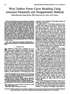
Figure 5. Wind speed bins and the Weibull fit.

The measured wind speeds divided into similar speed bins as seen in Figure 5. The integral eq.(30) calculated using the standard approximate rectangle method 50

E

T

pr (n) Pw(n)

(31)

n 0

where n is the number of the speed bin. Figure 6. Tower height wind speed data. 7. WIND DATA DESCRIPTION The wind data used in this article is measured using LIDAR equipment in Lappeenranta, southeastern Finland. The device measured wind speeds at 20 meter height intervals each second. The maximum height used is 200 meters. The LIDAR data contains several blanks and other clear errors, which is filled with measured wind data from a nearby TV tower. A data period of 168 hours from 17 to 23 Oct 2010 is selected since it

The dynamic simulation uses the data directly as a time series. With a one-second sampling time, the time series has 604 800 samples. For the power curve calculation, the wind velocity distribution has to be extracted from the data. While the most commonly used distribution for wind data is the Weibull distribution, it does not fit the emergent omni-directional wind distribution well, as seen in Figure 5. This is likely due to the short measurement period. For this reason, it is decided to use

the emergent calculations.

distribution

for

the

power-curve-based

10. REFERENCES [1]

8. COMPARISON OF POWER CURVE WITH DYNAMIC SIMULATION MODEL

[2]

One of the objectives of the study was to compare two methods of calculating wind turbine energy production. The power curve calculation method is used by most WSD tools, and can therefore be taken as the base method. However, the results obtained with the studied dynamic model of the turbine are more realistic, since the change of the wind speed with height, ignored by the first model, is essential to the final result.

[3]

The basic method, which uses the power curve, showed that the wind turbine energy production for given wind conditions over the investigated time interval of one week is 72.43 MWh. The analysis of the same input conditions by the dynamic model identifies produced energy at the rate of 75.03 MWh representing the difference of 3.5%. The difference of 3.5% in terms of economics, using the proposed 83.5€/MWh [12] feedin tariff for wind turbines and estimating the real annual capacity-hours to be about the typical 2400h [7], the production difference obtained is about 3000€/turbine/year, or about 600000€ for the 20 year usable life of a small 15 MW wind farm. Thus, the use of the basic method may produce a large error when designing the installation of a windmill.

[6]

There are several reasons for this. Firstly, the dynamic model takes into account the change in wind speed with height and the associated asymmetrical distribution of energy produced by individual blades of the turbine rotor depending on their position in the vertical plane of rotation. This phenomenon of sharp wind speed change with height is significant in areas with complex terrain, such as in Finland with its complex terrain and large areas of forested land. Secondly, the dynamic model with its unsteady BEMM takes into account the transient processes occurring with spontaneous changes in wind speed. But when using the power curve it is assumed that the turbine power changes instantly according to the wind. 9. CONCLUSIONS This paper presents a wind turbine model created in the Simulink environment. The unsteady BEMM constitutes the core of the dynamic model. It takes into account the transient processes occurring with inconstant changes of the wind speed. The global clusters include wind turbine aerodynamic calculations, basic structural mechanics, generator model, and controllers. The developed model allows to take into account instability in the wind speed distribution with height. To determine the adequacy of the dynamic model, it is compared with the classical technique based on power curve calculations generated artificially. The analysis is based on the data of actual one-week wind speed observations near the town of Lappeenranta, Finland in October 2010.The aerodynamical and mechanical information required for calculation was determined based on the WindPACT 1.5 MW wind turbine. A comparative analysis shows that the estimated energy output determined by the dynamic model is 3.5% more than the one determined by the power curve method. Hence, it can be argued that when considering wind turbine projects, one should use a dynamic model in order to obtain adequate results without neglecting the wind speed distribution with height as well as dynamic behavior of wind speeds. Ultimately, this has a significant influence on the decision of wind turbine installation.

[4]

[5]

[7]

[8] [9] [10] [11]

Manwell J.F., McGovan J.G., Rogers A.L. Wind Energy Explained, 2nd Edition, Wiley, 2009. IEC 61400-12-1 Ed.1: Wind turbines - Part 12-1: Power performance measurements of electricity producing wind turbines. Hansen M.O.L. Aerodynamics of Wind Turbines, 2nd Edition, London: Earthscan, 2008 Valtanen Esko, Tekniikan taulukkokirja, 14th edition, Jyväskylä, Genesis-kirjat Oy, 2007 [Handbook of technical formulas] (in Finnish) Bywaters G., John V. et al. Northern Power Systems WindPACT Drive Train Alternative Design Study Report, 2005 Tiainen R. Utilization of Time Domain Simulator in the Technical and Economic Analysis of a Wind Turbine Electric Drive Train, LUT Energy, Lappeenranta University of Technology, Lappeenranta, 2010 VTT Technical Research Centre of Finland Tuulivoiman tuotantotilastot vuosiraportti 2009, VTT-WORK-145, 2010 [Wind energy statistics of Finland, Yearly report 2009], (in Finnish) Tedric A . Harris and Michael N . Kotzalas, Essential Concepts of Bearing Technology, Fifth Edition, CRC Press, 2007, ISBN 978-1-4200-0659-9 Garrad Hassan and Partners Ltd GH WindFarmer 4.1 Theory Manual, 2010 Mortensen N.G., Heathfield D.N., Rathmann O. and Nielsen M. Wind Atlas Analysis and Application Program: WAsP 10 Help Facility, 2009 Finnish Government Hallituksen esitys Eduskunnalle laiksi uusiutuvilla energialähteillä tuotetun sähkön tuotantotuesta, HE 152/2010, 2010 [Government Bill on production support for electricity produced with renewable sources of energy], (in Finnish)