Modeling the magnitude and spatial distribution of ... - Semantic Scholar

Environment and Planning B: Planning and Design 2007, volume 34, pages 121 ^ 138

DOI:10.1068/b30101

Modeling the magnitude and spatial distribution of aesthetic impacts Denis J Dean, Alicia C Lizarraga-Blackard

Department of Forest Sciences, 113 Forestry Building, Colorado State University, Fort Collins, CO 80523, USA; e-mail: [email protected] Received 27 November 2003; in revised form 21 December 2005

Abstract. Timber-harvesting operations, especially clearcutting (that is, harvesting operations where all of the trees in a given area are removed), have been criticized for many reasons, not least of which is their unsightly appearance. Forest managers have recognized this, and have attempted to place clearcuts in locations with limited viewsheds. In order to find such locations, forest managers have made extensive use of standard geographical information system (GIS) viewshed operations. The use of conventional viewshed operations ignores the possibility that the aesthetic impacts of clearcuts might be diminished by the screening effects of intervening vegetation, or the possibility that impacts simply decrease with increasing distance. In this study we found evidence that the aesthetic impacts of clearcuts do in fact diminish in these ways. Photograph transects were performed around ten clearcuts. Each transect produced a series of pictures showing the clearcut from increasing distances into the surrounding forest. The Law of Comparative Judgments (LCJ) technique was used to develop perceived-scenic-beauty rankings for each photograph. Statistical analyses showed aesthetic impacts do in fact diminish with viewing distance through screening vegetation. A modified viewshed algorithm was then developed not just to identify areas where clearcuts are visible, but also to map localized aesthetic impacts of clearcuts. The approach presented here could be used to develop similar models that map the aesthetic impacts of any proposed environmental modification.

Introduction Scenic beauty has been recognized as an important factor in forest management for at least the past four decades. For example, in the United States, the National Environmental Policy Act of 1969, the Multiple-Use Sustained-Yield Act of 1960 and the National Forest Management Act of 1976 all require the US Forest Service to consider aesthetics along with wildlife, recreation, wilderness resources, and other factors as important components of national forest management. Legislative actions such as these, along with increased public concern for forest aesthetics, have encouraged forest managers to consider the aesthetic impacts of their activities and prompted researchers to explore the topic of public perception of the aesthetic impacts of forest-management activities (Bishop and Karadaglis, 1997; Erdle, 1999). Timber harvesting has greater impacts on forest aesthetics than virtually any other forest-management activity. Clearcutting, where virtually all the trees in a relatively large contiguous area are removed, has especially dramatic aesthetic impacts. At least in part because of these profound aesthetic impacts, clearcutting has become intensely controversial, and the economic, ecologic, sociologic, as well as aesthetic impacts of this practice have become the subject of heated debate (Kline and Armstrong, 2001; Limerick, 2002). While recognizing the importance of all of the consequences of clearcutting, in this paper we focus exclusively on the aesthetic impacts of the practice. Forest managers have long recognized the importance of addressing these aesthetic impacts, and their most frequent response has been to place clearcuts in areas with restricted viewsheds (Gustafson and Crow, 1998). Conventional GIS-based viewshed analyses are frequently used to find such locations. This strategy is obviously based on the intuitively sensible idea that by limiting the area in which a clearcut is visible, the overall aesthetic impact

122

D J Dean, A C Lizarraga-Blackard

of the clearcut will also be limited. In effect, this approach uses the extent of the viewshed of a clearcut as a proxy measure of the overall aesthetic impact of the clearcut. Note that, although on the surface this simple approach seems intuitively appealing, it is based on a very nonintuitive implicit assumption. Specifically, it assumes that all areas within the viewshed of a clearcut are impacted equally by the cut. It seems likely that the aesthetic impacts of clearcuts diminish with increased viewing distance and as a consequence of the screening effects of vegetation between the viewer and the clearcut. Research by Buhyoff and Wellman (1980) supports the hypothesis that the aesthetic impacts of clearcuts do in fact diminish as a result of these factors. If this hypothesis is true, merely identifying viewsheds is not an adequate way of measuring the aesthetic impact of clearcuts, because a clearcut with a large but lightly impacted viewshed might actually have less overall aesthetic impact than an alternative clearcut with a smaller but highly impacted viewshed. A more complete measure of aesthetic impact would differentiate between areas within the viewshed that are heavily impacted and other areas that are less heavily impacted. The purpose of this study is to investigate how screening vegetation affects the magnitude and spatial distribution of the aesthetic impacts caused by clearcuts, and to develop a GIS-based model to estimate these impacts across the landscape. It was hypothesized that the perceived aesthetic impacts of a clearcut are at their maximum along the edge of the cut, and that these impacts decrease as a function of distance from the cut. It was further hypothesized that the rapidity of this decrease is influenced by the amount and type of screening vegetation present. At some point, the impacts go to zero as the cut either becomes invisible or becomes an insignificant part of the visible landscape. This basic hypothesis seems equally plausible in other situations where an aesthetically unappealing locationöindustrial or other development, other natural-resource extraction operations (such as mining), and so forthöis sited within an aesthetically pleasing environment that acts as a screen around the unappealing location. An extensive body of literature exists describing how the relative perceived scenic beauty of a series of landscapes can be measured (Arthur, 1977; Brown and Daniel, 1986; Daniel and Boster, 1976; Hull et al, 1984; Ribe, 1990). These measurement techniques typically involve individuals rating a series of photographs representing the landscapes being compared. The end result of these comparisons are a series of interval-scale landscape preference ratings. In this paper, these techniques were used to measure the perceived scenic beauty of a series of landscape photographs taken at various distances, and through varying degrees of intervening vegetation, from clearcuts. Regression analyses were performed on these rankings to determine if the expected relationship existed between perceived scenic beauty and viewing distance or extent of screening vegetation. The results of these regression analyses were incorporated into a predictive GIS model. This model extended existing GIS viewshed techniques to include calculating viewing distance through screening vegetation before reaching a clearcut. These measures could then be incorporated into the regression equations to estimate the relative aesthetic impact of the clearcut at any point in the surrounding landscape. Previous research Over the past forty years, aesthetic preferences toward forested landscapes have been examined in many studies. In most of these studies there has been a differentiation between `near-view' and `vista' landscapes. Near-view scenes consist of forest landscapes within 100 ^ 200 yards of an observer and depict the viewer's experiences

Modeling the magnitude and spatial distribution of aesthetic impacts

123

`within' the forest, whereas vista scenes involve distant landscape features such as mountains or overlooks. The nature of aesthetic reactions to these two types of landscapes have been found to be quite different, and hence models developed for one type of landscape should not be generalized to the other (Brown and Daniel, 1986). Under this dichotomy, we focused exclusively on near-view landscapes and hence our results should not be generalized to vista-type landscapes. Several studies have related forest-inventory and forest-management attributes to perceived scenic beauty. Arthur (1977) found relationships between scenic beauty and tree species, tree size, amount of downed wood, tree density (number of trees per acre), and basal area (total square footage of the cross sections of all of the trunks of trees growing on a particular acre of ground), as well as a number of factors relating to the design of the photographs themselves (for example, lighting, position, detail). Using near-view models, Rudis et al (1988) found a positive association between scenic beauty and visual penetration through sawtimber-sized trees and a negative relationship between scenic beauty and vision-obscuring foliage, twigs, and sapling-size trees. Ribe (1990) evaluated several physical factors such as downed wood, tree density, size, mortality, and species and found that tree mortality had the greatest impact on scenic beauty preferences. This finding was in agreement with earlier work by Buhyoff and Leuschner (1978) and Buhyoff et al (1982), who found strong relationships between the amount of visible insect-caused tree mortality and scenic quality of both vista and near-view landscapes. Hollenhorst et al (1993) confirmed this result by finding that the percentage of trees killed by gypsy moths was a significant predictor of near-view forest scenic beauty. Virtually all of the preceding studies have utilized one of two methods of quantifying scenic beauty. These methods are the Scenic Beauty Estimation Method (SBE) developed by Daniel and Boster (1976) and the Law of Comparative Judgment (LCJ) introduced by Buhyoff and Leuschner (1978), who built on the work of Thurstone (1927). Both methods produce indices based on perceptions of the scenic beauty of a series of photographs representing a landscape, and both methods have been extensively tested and validated (Hull et al, 1984). The SBE technique involves a scaling procedure where each respondent utilizes a scale (usually from 1 to 10) to subjectively rate the scenic beauty of a series of photographs. The LCJ method requires each respondent to compare all possible pairs of photographs and decide which photograph in each pair is more scenic. The two procedures are described and compared in detail by Hull et al (1984). In general, the SBE method is more efficient than the LCJ approach, in the sense that each individual evaluating n photographs under the SBE method need only make n ratings. Under the LCJ approach, the same n photographs require n (n ÿ 1)=2 comparisons of photograph pairs. As under most conditions the efficient SBE method has been found to be just as accurate and reliable a predictor of scenic-beauty preferences as the more labor-intensive LCJ approach, the SBE method has become the preferred approach to scenic-beauty estimation (Daniel and Boster, 1976). However, there is one exception to this general preference for the SBE approach. When the photographs being compared are very similar to one another (thereby requiring the evaluators to make fine distinctions between photographs with similar scenic qualities), the use of all possible pairs of photographs in the LCJ approach offers distinct advantages over the SBE method (David, 1988; Hull and Buhyoff, 1981). In many instances within this paper, evaluators were asked to compare the relative beauty of scenes that differed only by their distances from clearcuts. It was believed that under these conditions, the LCJ approach was more appropriate than the SBE method. Thus, the LCJ approach was used throughout this paper.

124


Methods Study area

Clearcuts from two widely separate study areas were evaluated in this project. Five clearcuts were evaluated from the first study area; a southern yellow pine plantation located in the coastal plain of South Carolina (bottom portion of figure 1). The area was intensively managed for the commercial production of pulpwood (this involves growing relatively small trees suitable for the production of paper products). It consisted of homogeneous forest stands (that is, within each stand, there was very little variation in species composition, basal area, height, density, volume, or number of trees per acre). All stands had a very dense understory; that is, there were a great many tall grasses and shrubs growing underneath the trees. There was virtually no vertical relief in the area, with all slopes less than 2%. Two of the clearcuts from this area were surrounded by loblolly pine (Pinus taeda L.) stands, whereas the remaining three were surrounded by stands of hardwoods composed primarily of sweetgum (Liquidambar styraciflua L.), red maple (Acer rubrum L.), various oaks (Quercus spp.) and elms (Ulmus spp.), yellow-poplar (Liriodendron tulipifera L.), and hickories (Carya spp.).

ÿ10 0 10 20 30 40 km

Figure 1. Colorado (top) and South Carolina (bottom) study sites.


125

The second study site was located in the Colorado State Forest located in the Rocky Mountain Front Range (top portion of figure 1). Vegetation was predominantly lodgepole pine (Pinus contorta) with interspersed quaking aspen (Populus tremuloides) and spruce/fir (Picea engelmanii, Abies lasiocarpa) stands. Understory in these stands was much less dense than that found in South Carolina. The topography included steeper slopes, ranging from 17% to over 40%. A total of five clearcuts in Colorado were evaluated, with three surrounded by lodgepole pine stands, one by spruce/fir, and one by aspen stands. Site inventory procedure

A photograph transect was established in the forest adjacent to each clearcut. Each transect was a straight line starting at the edge of the clearcut and moving into the surrounding forest along a line extending out radially from the approximate center of the cut (figure 2). The specific orientation of the transect was randomly chosen; however, this process was frequently constrained because transects with certain orientations were obviously obstructed by intervening terrain or caused the transect to pass into two or more stands with obviously differing visual characteristics (for example, a mature aspen stand and an immature spruce/fir stand). In these cases, transect orientation was randomly selected from the set of orientations that did not encounter obstacles or pass into multiple forest stands. Starting at the edge of each clearcut, photographs of the cut were taken every 10 m along the transect until the clearcut was no longer visible. Once the cut was lost to view, an additional three photographs (covering 30 m) were taken to ensure that no sign of the clearcut was visible. A standard 35 mm camera with a 55 mm lens and ASA Stand 3 Stand 7 Stand 8 10 nd Sta

Stand 4

Hill

Stand 2

Clear cut

Stand 12

Random transect

Approx. center of clearcut

Azimuths disallowed owing to hill and multiple stands

Stand 9

Stand 5

Stand 13

Stand 6

Stand 14

Figure 2. Layout of a photograph transect around a hypothetical clearcut.

126


(a)

(c) Figure 3. Examples of photographs from the South Carolina and Colorado study sites. (a) Photograph taken 0 m from edge of South Carolina clearcut; (b) photograph taken 20 m from edge of South Carolina clearcut; (c) photograph taken 60 m from edge of Colorado clearcut; (d) photograph taken 140 m from edge of Colorado clearcut.

400 print film were used. All photographs were taken at the highest depth of field possible while maintaining a shutter speed of 1/60. All pictures were taken between 8 AM and 5 PM to guarantee sufficient light and no overwhelming shadows. To eliminate possible biases, every effort was made to ensure that no additional clearcuts, buildings, people, wildlife, or vehicles were photographed. In addition, photography was limited to the summer season to prevent any bias due to seasonal changes (Buhyoff and Wellman, 1980).


127

(b)

(d) Figure 3 (continued).

In addition to the photograph transects, field procedures also included taking tree measurements at a randomly selected point along each transect line. These measurements were taken using common forest inventory techniques. A 0.10 acre plot was established and the number of trees, average height of codominant trees (that is, the trees that make up the canopy of the forest), and the diameter at breast height (DBH, a standard measure of tree girth) of all trees with DBH greater than 3 inches was recorded. Understory and ground cover were noted but were not quantifiably measured. Aesthetic preference measurement

The LCJ technique was used to rate the scenic beauty of the photographs. LCJ requires a series of evaluators to select the more aesthetically pleasing photograph in each of a series of photograph pairs. This preference information is used to develop an interval-level scale of the relative attractiveness of each photograph.

128


Six 466 inch color photograph prints were used to represent each transect. Each set of six photographs started with the photograph taken at the edge of the cut and concluded with a photograph taken from a point at which the cut was no longer visible. The remaining four photographs were randomly selected from all usable photographs from each transect (a few photographs were eliminated from consideration because of poor focus, blurring, and so on). These photographs depicted the progression along the transect from the edge of the clearcut to the point where the cut was no longer visible. Distances between photographs ranged from 10 m to 50 m, and the maximum distance from the edge of the clearcut to the farthest photograph ranged from 90 m to 180 m. Examples of photographs from representative transects from both the South Carolina and Colorado study sites are shown in figure 3. The photographs from each transect were arranged into ten separate photograph albums containing the six prints arranged in all possible pairs (fifteen pairs per transect). The photographs were ordered in an optimum balancing routine (Ross, 1934) in which each photograph appeared an equal number of times on the top and on the bottom of the page as well as being proportionally distributed from the beginning to the end of the album. Subjects for evaluating the photographs were Colorado State University students and faculty and other Colorado professionals ( n 110) varying in age, profession, interest, and ethnic background. Prior to rating the photographs, a standard set of instructions was read to the subjects; no additional information beyond these instructions was provided. Each subject was presented with a photograph album and asked to indicate which photograph they preferred in each pair. They were allowed 5 ^ 8 s to select their preferred photograph from each pair. To minimize the possibility of fatigue, each subject only evaluated six (three from each study area) rather than all ten albums. Thus, each individual rated a total of ninety pairs of photographs (fifteen photograph pairs per transect 6 six transects). Statistical analysis

Data from the evaluations of each photograph transect were analyzed separately. The results of each transect were analyzed using the methodology presented by Guilford (1954, pages 154 ^ 177). Only data from evaluators who were consistent in their preferences were used in the final analysis. Consistency was determined by examining each evaluator's preferences. For example, if an evaluator preferred photograph A over photograph B and photograph B over photograph C, this evaluator cannot prefer photograph C over photograph A. Kendall (1962) termed inconsistencies such as these between three photographs `circular triads'; when the number of photographs is larger than three, an inconsistency is referred to as a circular n-ad. Inconsistencies may be a result of guessing or may be caused by the fact that the photographs being compared are indistinguishable. In this paper, the photographs varied only in distances from the clearcuts, and in some cases the photographs were almost identical. Although each transect was initially evaluated by sixty individuals, the number of consistent evaluations per transect ranged from twenty four to thirty nine. Once the preference data from the consistent evaluators for a given transect were identified, they were used to develop an interval-level scale of the attractiveness of each photograph. This was accomplished by calculating the observed probability that each photograph A would be preferred over photograph B for all pairs of photographs. Guilford (1954) terms the diagonally symmetric matrix showing all of these observed probabilities a dominance priority matrix. Following Guilford's procedures, the probabilities in the dominance priority matrix were then normalized


129

to produce Z scores for each probability, and these Z scores were then averaged to construct the estimated aesthetic ranking for each photograph. The standard LCJ procedure just described produced what we termed `raw' aesthetic-quality rankings. These raw aesthetic-quality rankings were entirely consistent with one another within a single transect, but owing to their interval nature, were not comparable across transects. In order to make between-transect comparisons, we standardized the raw scores so that the minimum ranking of each transect was zero and the maximum ranking was one. Given the interval scale of aestheticquality rankings, this standardization was accomplished without losing any of the information contained in the original LCJ results. We termed these standardized rankings. Thirteen separate datasets were constructed from the standardized rankings and were analyzed via regression analyses. The first ten datasets were specific to individual transects; each of these datasets were based on only six observations (representing the six photographs evaluated in each transect). Each of these datasets consisted of a single dependent variable (the standardized rankings of the photographs) and a single independent variable (the distance from the point where the photograph was taken to the edge of the clearcut). Two additional datasets were constructed by (1) aggregating all the data from the South Carolina transects, and (2) aggregating all the data from the Colorado transects. Each of these state-specific datasets were based on thirty observations (six observations/transect 6 five transects per state). In addition to the dependent and independent variables found in the ten transect-specific datasets, the two state ^ state specific datasets contained the forest-inventory measurements (tree density, DBH, average height of dominant and codominant trees, and a series of binary indicator variables used to identify species) measured along each transect as additional independent variables. Finally, an overall dataset was constructed by aggregating data from all ten transects across both states; this dataset contained sixty observations. This overall dataset contained the same dependent and independent variables as found in the state-specific datasets. Five intrinsically linear regression forms (true linear, squared, quadratic, exponential, and logarithmic) were used to analyze each of the thirteen analyses just described. These forms were chosen because Buhyoff and Wellman (1980) and Hull and Buhyoff (1983) used them in previous studies that related perceived scenic beauty to forest characteristics and viewing distance. In addition, a nonlinear regression equation was developed for each of the thirteen datasets described previously. Thus, a total of seventyeight regression results were produced (thirteen datasets 6 six regression forms per dataset). GIS-based spatial modeling

The results of the regression analyses just described were used to develop a model designed to estimate the aesthetic impacts of clearcuts on surrounding areas. The model was an extension of a modified GIS-based viewshed analysis technique proposed by Dean (1997). Standard viewshed analysis is binary; either the line of sight connecting a viewpoint to a raster cell is completely unobstructed (meaning the raster cell is entirely visible from the viewpoint) or completely obstructed (meaning that the raster cell is entirely invisible from the viewpoint) (Burrough, 1986; Laurini and Thompson, 1992; Tomlin, 1990). However, numerous authors have proposed nonbinary alternative viewshed estimation systems. A partial list of these alternative techniques includes probabilistic approaches (which create a raster surface where each cell contains the probability that it is visible from the viewpoint) (Fisher, 1992; 1994; Nackaertes et al, 1999), partial-cell approaches (which predict what proportion of each raster cell

130


is visible) (Sorenson and Lanter, 1993), and a system designed to account for the vision-obscuring effects of vegetation proposed by Dean (1997). The modified viewshed-delineation system proposed by Dean (1997) classifies raster cells into three categories: (1) completely visible (the line of sight from the viewpoint to the raster cells suffers from no obstructions, either topographic or vegetative), (2) completely invisible (the line of sight is entirely obstructed by one or more opaque topographic features), or (3) partially visible, meaning that the line of sight is not obstructed by opaque terrain but does pass through some distance of vegetation. For raster cells falling into the third category, the modified viewshed technique also computes the total length of the line of sight passing through vegetation. Using the modified viewshed system just described, the results of the regression analysis could be used to estimate the aesthetic impacts of clearcuts. In concept, this model iteratively places a viewpoint on each cell in the DEM. If the line of sight from this viewpoint to the clearcut is completely obstructed [that is, falls into case (2)], the clearcut has no aesthetic impact on the viewpoint cell so the viewpoint is assigned an aesthetic-impact rating of zero. If the line of sight is completely unobstructed [that is, falls into case (1)], the viewpoint cell is assigned a maximum aesthetic-impact rating of one. Finally, if the line of sight is partially obstructed [case (3)], the system computes the distance that the line of sight travels through the intervening forest vegetation prior to reaching the clearcut. This distance estimate is then used in the regression equation discussed previously (along with the forest inventory measures of the forest through which the line of sight is passing) to produce an estimated aesthetic impact rating for the cell. Results, validation, and discussion Relationship between aesthetic quality and viewing distance through forest

The ten transect-specific datasets were analyzed using the six regression models shown here (Y standardized scenic beauty ranking, X distance to clearcut, b0 , b1 , and b2 are regression parameters, and A is the asymptote for the nonlinear regression): Linear:

Y b0 b1 X ,

Square:

Y b0 b1 X 2 ,

Quadratic:

Y b0 b1 X b2 X 2 ,

Exponential: Y b0 b1 expX , Logarithmic: Y b0 b1 lnX , Nonlinear:

Y A1 ÿ expb0 b1 X .

All regression parameters for the five intrinsically linear models were estimated using standard parametric least-squared techniques, whereas the nonlinear regression parameters were estimated using the secant method (SAS, 1990). These analyses revealed that the logarithmic model proved to be significant at the 0.05 level and produced R 2 values greater than 0.7 for nine of the ten transects. The nonlinear, quadratic, square, and linear models were each significant at the 0.05 level for three transects, and the exponential model was significant for one transect (table 1). Similar analyses (using the same six regression forms) were also performed on the two datasets aggregated to the state level, but these analyses included the forest inventory measures as additional independent variables. A stepwise process was used to identify the set of independent variables that (1) were each significant predictors of the aesthetic ratings of the photographs and (2) collectively produced the highest


131

overall predictive power of all possible sets of independent variables. This process started with all independent variables in the model and then iteratively removed or added variables to the model until no further removals or additions that improved the model were available. The standardized rankings used as the dependent variables in these analyses were adjusted so that the single photograph within each dataset with the highest raw ranking was given a value of one (rather than the highest-ranked photograph from each individual transect being given a ranking of one) and the single photograph with the lowest raw ranking was given a value of zero. Results from both states were very similar. For both states, five of the six regression models were significant at the 0.05 level; only the exponential model was insignificant. The nonlinear model provided the highest pseudo R 2 of the five significant models, followed by the logarithmic model (table 1). A somewhat unexpected finding resulted from the stepwise independent-variable selection procedure. For each of the six regression models investigated from both states (a total of twelve models), the only independent variable that was retained in each of the final models was distance from the photograph to the edge of the clearcut; none of the forest-inventory measures were significant. In retrospect, the reason why forest inventory measures were insignificant predictors of aesthetic preference was obvious. The South Carolina study site featured very flat terrain. Given the flat terrain, lines of sight generally passed under the forest canopy and thus were effected much more significantly by the understory vegetation than they were by the overstory forest trees. As the forest inventory measures evaluated in this paper pertained only to the overstory, it would have been surprising if these measures were related to aesthetic preference. In the Colorado study site, a subjective examination of the photographs shows that understory still played the more obvious role but, given the rolling terrain, it is certainly plausible that at least some lines of sight could have been impacted by the overstory. The fact that none of the regression analyses described in table 1 found any of the overstory inventory measures to be significant predictors of aesthetic impact implies that if such overstory effects took place, they were not significant enough to be retained in the regression models. Some of the stands in the Colorado study areas were composed of very densely packed small trees (that is, `doghair' stands), and it seems likely that the density of tree boles in these stands could impact even lines of sight passing under the forest canopy. However, no single inventory measure could identify these doghair standsöidentifying these stands required evaluation of the combined values of all three inventory measures. Thus, the Colorado dataset was analyzed again using a stepwise regression procedure that considered as potential independent variables not only distance and the overstory inventory measures evaluated previously, but also all four possible interactions of the continuous inventory measures (trees per acre 6 height, trees per acre 6 mean DBH, height 6 mean DBH, and trees per acre 6 height 6 mean DBH). Once again, all six forms of the regression model were evaluated. In each of these six analyses the three-way interaction of trees per acre 6 height 6 mean DBH was found to be a significant predictor of aesthetic preference, but the addition of this interaction variable did not noticeably improve the R 2 values of the resulting regression models. The linear model showed the greatest improvement, with its R 2 value increasing from 0.3114 without the interaction variable to 0.3202 with the interaction variableö an increase of only 0.0088. Given the very small magnitude of this improvement, it was decided to remove the forest inventory measures from all of the remaining analyses.

132


Table 1. Results of the regression analyses, for each individual transect, each study site, and both study sites combined. NCRa

Transect 1 Transect 2 Transect 3 Transect 4 Transect 5 Transect 6 Transect 7 Transect 8 Transect 9 Transect 10 CO only SC only CO and SC

14 21 15 27 14 22 28 29 27 25 98 124 222

n

6 6 6 6 6 6 6 6 6 6 30 30 60

Exponential

Linear

R2

p

R2

p

0.2548 0.1615 0.9519 0.0001 0.3127 0.2358 0.2826 0.0092 0.0352 0.0692 0.0158 0.0581 0.0312

0.3072 0.4297 0.0009 0.9902 0.2486 0.3289 0.2778 0.5631 0.7220 0.6146 0.5076 0.1996 0.1770

0.7700 0.5153 0.5514 0.1987 0.6101 0.8437 0.9245 0.4938 0.7171 0.4655 0.3114 0.4135 0.3203

0.0216 0.1082 0.0909 0.3756 0.0666 0.0097 0.0022 0.1194 0.0334 0.1354 0.0014 0.0001 0.0001

a NCR number of consistent ratings. This is the number of individuals who consistently rated the photographs in each transect. This should not be confused with the sample size (n).

The same six regression models were applied to the overall dataset created by combining data from all ten transects. Once again, the standardized rankings in this final dataset were adjusted so that the single photograph with the highest raw ranking was given a value of 1 and the photograph with the lowest raw ranking was given a value of 0. The results from this final dataset were very similar to those obtained with the previous two datasets: five of the six models produced significant results at the 0.05 level, with the nonlinear and logarithmic models producing the highest R 2 values. Only the exponential model produced insignificant results. Regression model validation

The results shown in table 1 indicate that the logarithmic and nonlinear regressions generally outperformed (in terms of R 2 and p-values) the other regression models. In addition, table 1 indicates that models aggregated at the state level tended to outperform models aggregated across both states; this may be because of the obvious dissimilarities in the screening capabilities of the forests in the two states. These findings implied that in the second phase of this study, the predictive model designed to estimate the aesthetic impacts of clearcuts should be based on data aggregated at the state level and logistic and nonlinear regression forms should be considered. However, prior to developing such a predictive model, the predictive power of these two regression models was evaluated using a pair of bootstrapping processes. Each bootstrapping process involved removing the data from one transect from a state level database. This produced a reduced dataset containing information from four transects. Logarithmic and nonlinear regression analyses were then used to produce regression results from this reduced dataset. These reduced regression results were then used to derive estimated aesthetic rankings for photographs taken at each of the six distances from clearcuts contained in the removed transect. These estimated aesthetic rankings were then compared with the observed standardized rankings contained in the removed transect, and differences between actual and predicted rankings were noted. This process was then repeated by removing a different transect from the original database, until each transect had been removed once.


133

Table 1 (continued). Square

Quadratic

Logarithmic

Nonlinear

R2

p

R2

p

R2

p

R2

p

0.5484 0.3607 0.7644 0.0537 0.4232 0.7121 0.7573 0.2942 0.4757 0.2550 0.1451 0.2300 0.1750

0.0923 0.2074 0.0227 0.6586 0.1618 0.0347 0.0242 0.2662 0.1297 0.3069 0.0378 0.0073 0.0009

0.8679 0.6422 0.8909 0.6473 0.7436 0.8710 0.9598 0.7267 0.9840 0.8694 0.5520 0.5054 0.4309

0.0742 0.2221 0.1591 0.1103 0.1482 0.1503 0.0301 0.1175 0.0023 0.0329 0.0001 0.0006 0.0001

0.8175 0.9107 0.0902 0.7502 0.8736 0.7735 0.8065 0.9495 0.7053 0.9508 0.5188 0.7786 0.5482

0.0133 0.0031 0.5630 0.0257 0.0063 0.0209 0.0151 0.0010 0.0364 0.0009 0.0001 0.0001 0.0001

0.8932 0.8962 0.9779 0.9148 0.8622 0.8722 0.9661 0.9682 0.9301 0.9674 0.9947 0.9976 0.9983

0.0993 > 0:1 0.0218 >0.1 >0.1 >0.1 0.0765 0.0240 0.0720 0.0480 0.0183 0.0122 0.0014

The results of the bootstrapping analysis are shown in table 2. The logarithmic regression model resulted in an average mean difference (observed value minus predicted value) of 0.0674 for the Colorado study site (differences range from ÿ0.4476 to 0.4170) and an average mean difference of 0.0898 for the South Carolina study site (range ÿ0.4621 to 0.3040). The nonlinear regression model resulted in an average mean difference of ÿ0.0008 for the Colorado site (range ÿ0.3657 to 0.4125) and ÿ0.0038 for the South Carolina site (range ÿ0.3192 to 0.2729). It is interesting to note that six of these eight extreme values were recorded at zero distance from the clearcut; if these zero-distance estimates are ignored, the overall performance of both models improved significantly. When evaluating these deviations it is helpful to recall that all rankings were standardized to range from zero to one, so an average difference of 0.09 indicates that average differences covered 9% of the possible range of standardized rankings. Clearly, both the logarithmic and nonlinear models produced estimates that on average were fairly close to observed values, but again on average the nonlinear model outperformed the logarithmic model. Aesthetic impact model

Given that they outperformed all of the other regression models, both the logarithmic and nonlinear regression equations were used in building a GIS-based aesthetic impact model. As the regression models failed to include anything other than distance as an independent variable, there was no need to include any forest inventory measures in the aesthetic-impact model. The aesthetic-impact model was tested for logical consistency by applying it to several artificial datasets based on simple elevation surfaces. The overall results produced by the model seem intuitively reasonable, and cell-by-cell examination of these results showed the expected patterns: raster cells immediately adjacent to the clearcuts showed the greatest level of impact, and the magnitude of impacts decreased as viewing distance increased. Raster cells where the clearcut was completely hidden by intervening terrain showed no aesthetic impact.

134


Table 2. Bootstrap results (observed rating ÿ predicted rating) for (a) Colorado and (b) South Carolina. Bootstrap results at (distance from clearcut in meters): 0

10

20

30

40

(a) Colorado study site Logarithmic model Transect 1 0.0193 Transect 2 0.2839 Transect 3 ÿ0.3178 Transect 4 ÿ0.4476 Transect 5 ÿ0.0631 Mean ÿ0.1051 Minimum ÿ0.4476 Maximum 0.2839

0.1139 0.0542 ÿ0.0942 ÿ0.1208 ÿ0.0117 ÿ0.1208 0.1139

Nonlinear model Transect 1 0.1346 Transect 2 0.4125 Transect 3 ÿ0.2271 Transect 4 ÿ0.3657 Transect 5 0.0467 Mean 0.0002 Minimum ÿ0.3657 Maximum 0.4125

ÿ0.0356 0.1394 0.0841 0.1678 0.0154 ÿ0.1042 ÿ0.0751 ÿ0.1329 ÿ0.0034 0.0661 ÿ0.0299 ÿ0.1329 ÿ0.0356 ÿ0.0751 0.1394 0.1678 0.0154

50

0.0264 0.1874

60

0.0230 0.0686

0.0700 ÿ0.0012

0.1059 0.1082 0.0764 0.0230 0.1082

0.1069 0.0344 0.0264 ÿ0.0012 0.1874 0.0700

70

0.0648 0.0648 0.0648 0.0648

80

0.3503 0.3503 0.3503 0.3503

ÿ0.1161 ÿ0.0882

ÿ0.0461 0.0109 ÿ0.0187 ÿ0.0530 ÿ0.0461 ÿ0.1161 ÿ0.0461 0.0109 ÿ0.0461

0.2497 0.2497 0.2497 0.2497

Mean deviation for the logarithmic model 0.0674. Mean deviation for the nonlinear model ÿ0.0008. (b) South Carolina site Logarithmic model Transect 1 ÿ0.4621 Transect 2 ÿ0.0701 Transect 3 0.0865 Transect 4 ÿ0.3584 0.0596 Transect 5 ÿ0.0112 Mean ÿ0.1631 0.0596 Minimum ÿ0.4621 0.0596 Maximum 0.0865 0.0596 Nonlinear model Transect 1 ÿ0.3192 Transect 2 0.0960 Transect 3 0.2729 Transect 4 ÿ0.2115 Transect 5 0.1650 Mean 0.0006 Minimum ÿ0.3192 Maximum 0.2729

ÿ0.0054

0.2504 0.0319 0.1045 0.1289 0.0319 0.2504

0.1010 ÿ0.1414

ÿ0.0618 ÿ0.0054 ÿ0.0341 ÿ0.0054 ÿ0.1414 ÿ0.0054 0.1010

0.2130 ÿ0.0010 0.3040 0.1499 0.2130 0.1510 0.2130 ÿ0.0010 0.2130 0.3040 0.0745

0.1326

0.1203 0.2068 0.1399

0.1326 0.1326 0.1326

0.1557 0.1203 0.2068

0.0206 0.1685 0.1530 0.1140 0.0206 0.1685

ÿ0.0098 0.0406 ÿ0.1414 ÿ0.1778 0.0073 0.1587 0.0031 ÿ0.0250 ÿ0.0074 0.0745 ÿ0.0147 ÿ0.0378 0.0113 ÿ0.0472 0.0745 ÿ0.1778 ÿ0.0378 ÿ0.0098 ÿ0.1414 0.0745 0.1587 ÿ0.0378 0.0406 0.0073

Mean deviation for the logarithmic model 0.0898. Mean deviation for the nonlinear model ÿ0.0038.

0.1532 0.1532 0.1532 0.1532

ÿ0.0378

0.0232 0.0232 0.0232 0.0232


135

Table 2 (continued).

90

0.1414 0.0580

0.0997 0.0580 0.1414 ÿ0.0134 ÿ0.1310

ÿ0.0722 ÿ0.1310 ÿ0.0134

ÿ0.0178 0.0444 0.1411 0.0635 0.0578 ÿ0.0178 0.1411 ÿ0.1387 ÿ0.1107 ÿ0.0127 ÿ0.0896 ÿ0.0879 ÿ0.1387 ÿ0.0127

100

110

0.0560 0.3387 0.4170 0.1806 0.3121 0.1806 0.4170

0.0560 0.0560 0.0560 ÿ0.0997

120

0.1041 ÿ0.0264 0.0389 ÿ0.0264 0.1041

140

0.0375

0.0375 0.0375 0.0375

150

ÿ0.0642 0.1909 0.1909 0.1909 0.1909

ÿ0.1585

0.2097 0.3161 0.0455 0.1904 ÿ0.0997 ÿ0.1585 0.0455 ÿ0.0997 ÿ0.1585 0.3161 ÿ0.0997 ÿ0.1585

0.2287 0.1237 0.1762 0.1237 0.2287

130

ÿ0.0642 ÿ0.0642 ÿ0.0642

ÿ0.2592 0.0592 0.0590 0.0592 0.0592

160

170

180

0.1452

0.0906 0.1179 0.0906 0.1452 ÿ0.0058

ÿ0.0379 ÿ0.2592 ÿ0.0219 ÿ0.2592 ÿ0.0379 ÿ0.2592 ÿ0.0058

0.2270

0.3108

0.2270 0.2270 0.2270

0.3108 0.3108 0.3108

0.1180

0.2060

0.1180 0.1180 0.1180

0.2060 0.2060 0.2060

0.1812 0.1812 0.1812 0.1812

0.0334 0.0334 0.0334 0.0334

136


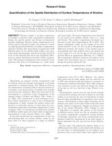
Predicted aesthetic impacts produced using the logarithmic equation were similar to those produced using the nonlinear equation. When the raster maps produced by the two equations were subtracted, it was found that in general, the nonlinear model produced slightly higher aesthetic-impact estimates than the logarithmic model at very small distances from the clearcut, but tended to produce lower-impact estimates at larger distances. Once the model had been tested on these artificial study areas, it was applied to real-world situations involving clearcuts from both the Colorado and South Carolina study sites but not used in the model-building process. A set of typical results from these analyses can be seen in figure 4. Clearcut A

Clearcut B

Area 916.83 ha Sum impact 385 870

Area 95.13 ha Sum impact 46 432 Clearcut C

Aesthetic impact High

Low Clearcut

Area 733.86 ha Sum impact 539 852

Figure 4. Results of aesthetic-impact estimation model when applied to real-world datasets.

It is interesting to view the results shown in figure 4 as if they were comparisons of proposed clearcuts. If you were using the standard viewshed approach to evaluate the cuts, you would conclude that cut A was the least objectionable (because it has the smallest viewshed), followed by cut C, with cut B being the most objectionable (that is, it has the largest viewshed). However, the aesthetic-impact model indicates that the large viewshed of clearcut B is mostly lightly impacted aesthetically, whereas the smaller viewshed of cut C is almost-entirely heavily impacted. This fact is reflected in the sum of impacts values shown in the figure. These values are simply the sum across all raster cells of the predicted aesthetic-impact values. Recall that a cell that is highly impacted has a large predicted aesthetic value whereas a cell that is not impacted at all has an aesthetic-impact value of zero. Thus, higher sums of impacts values reflect clearcuts that have greater overall impacts. Using this model, you would still conclude that A is the least objectionable clearcut, but then you would find cut B to be the next best alternative, with cut C being the least desirable.


137

Conclusions In this paper we have demonstrated that it is possible to combine the models that have been developed to quantify aesthetic preferences with the spatial modeling capabilities of GIS. The resulting hybrid has unique advantages that are not present in either conventional aesthetic preference models or off-the-shelf GIS software. It seems likely that a fully functional version of the hybrid model developed here could be of considerable worth to forest managers. Furthermore, it seems plausible that approaches similar to those used here could be adopted to other aesthetic impact situations öfor example, the impacts of the wind turbines investigated by Bishop (2002). In fact, there is no conceptual reason why the model developed here could not be extended to situations involving urban or other man-made environments. The only assumption made here is that an aesthetically unappealing site is located within a more appealing surrounding environment, and that the effectiveness of the surrounding environment at screening the unappealing site increases as one moves further away from the site. As long as this assumption is met, a model of the same basic type as that presented here could be used to estimate the impact of any aesthetically unappealing site. At least two issues remain to be resolved before a fully functional aesthetic-impact model could be constructed. First, we looked only at near-view impacts; this would obviously have to be married with a model that estimates impacts over longer viewing distances to produce estimates of total aesthetic impacts. Fortunately, there is no reason to believe that the techniques used in this study could not be extended to longer viewing distances. A cutoff distance (probably equal to the maximum length of transects like those used in this study) could be established, and a model identical to the one developed here could be used to estimate aesthetic impacts within this distance. Beyond this cutoff, photographs of clearcuts could be taken from longer distances and used in the SBE or LCJ approach to measure aesthetic preferences over vista-scale landscapes. Regression analyses could then be used to quantify the relationship between aesthetic quality and these longer viewing distances, and these regression results could be incorporated into GIS-based models to estimate aesthetic impacts over vista-scale landscapes. An obvious area where we failed in this paper was in relating changes in aesthetic preferences over distance to forest inventory measures. It is certainly possible that other overstory inventory measures not investigated in this paper might produce better results. However, based on subjective reviews of the photographs used in this paper, relating aesthetics to understory vegetation measures seems much more promising than any measure of overstory characteristics. Finally, it remains to be seen if the more efficient SBE method could be used in this sort of study rather than the LCJ approach adopted here. It is undeniably true that the SBE method is more efficient than the LCJ system and, in many other areas, the SBE method has been found to be just as precise and accurate as the LCJ approach. If this is found to be true for the transect sampling used in this study, the SBE method would be a very attractive alternative to the more labor-intensive LCJ system. Despite these limitations, the model developed in this paper fulfilled its purpose of demonstrating the feasibility of producing spatial aesthetic-impact models. The results presented here provide a starting point for further research in the development of linked LCJ, SBE, and GIS models designed to quantify and analyze the commutative aesthetic effects. References Arthur L M, 1977, ``Predicting scenic beauty of forest environments: some empirical tests'' Forest Science 23 151 ^ 160 Bishop I D, 2002, ``Determination of thresholds of visual impact: the case of wind turbines'' Environment and Planning B: Planning and Design 29 707 ^ 718

138


Bishop I D, Karadaglis C, 1997, ``Linking modelling and visualisation for natural resources management'' Environment and Planning B: Planning and Design 24 345 ^ 358 Brown T C, Daniel T C, 1986,``Predicting scenic beauty of timber stands'' Forest Science 32 471 ^ 487 Buhyoff G J, Leuschner W A, 1978, `Èstimating psychological disutility from damaged forest stands'' Forest Science 24 424 ^ 434 Buhyoff G J, Wellman J D, 1980, ``Seasonality bias in landscape preference research'' Leisure Science 2 181 ^ 190 Buhyoff G J, Wellman J D, Daniel T C, 1982, ``Predicting scenic beauty for mountain pine beetle and western spruce budworm damaged forest vistas'' Forest Science 28 827 ^ 838 Burrough P A, 1986 Principles of Geographical Information Systems for Land Resource Assessment (Oxford University Press, Oxford) Daniel T C, Boster R S, 1976 Measuring Landscape Aesthetics:The Scenic Beauty Estimation Method research paper 167, USDA Forest Service Rocky Mountain Research Station, Fort Collins, CO David H A, 1988 The Method of Paired Comparisons 2nd edition (Charles Griffin, London) Dean D J, 1997, `Ìmproving the accuracy of forest viewsheds using triangulated networks and the visual permeability method'' Canadian Journal of Forest Research 27 969 ^ 977 Erdle T A, 1999, ``The conflict in managing New Brunswick's forests for timber and other values'' Forestry Chronicle 75 945 ^ 954 Fisher P F, 1992, ``First experiments in viewshed uncertainty: simulating fuzzy viewsheds'' Photogrammetric Engineering and Remote Sensing 58 345 ^ 352 Fisher P F, 1994, ``Probable and fuzzy models of the viewshed operation'', in Innovations in GIS Ed. M F Worboys (Taylor and Francis, London) pp 161 ^ 175 Guilford J P, 1954 Psychometric Methods (McGraw-Hill, New York) Gustafson E J, Crow T R, 1998, ``Simulating spatial and temporal context of forest management using hypothetical landscapes'' Environmental Management 22 777 ^ 787 Hollenhorst S J, Brock S M, Freimund W A, Twery M J, 1993, ``Predicting the effects of gypsy moth on near-view aesthetic preferences and recreation appeal'' Forest Science 39 28 ^ 40 Hull B R, Buhyoff G J, 1981,`Òn the law of comparative judgement: scaling with intransitive observers and multi-dimensional stimuli'' Educational and Psychological Measurement 41 1083 ^ 1089 Hull B R, Buhyoff G J, 1983, ``Distance and scenic beauty: a nonmonotonic relationship'' Environment and Behavior 15 77 ^ 91 Hull B R, Buhyoff G J, Daniel T C, 1984, ``Measuring of scenic beauty: the law of comparative judgement and scenic beauty estimation procedures'' Forest Science 30 1084 ^ 1096 Kendall M G, 1962 Rank Correlation Methods 3rd edition (Hafner, New York) Kline J D, Armstrong C, 2001, `Àutopsy of a forestry ballot initiative: characterizing voter support for Oregon's measure 64'' Journal of Forestry 99 20 ^ 27 Laurini R, Thompson D, 1992 Fundamentals of Spatial Information Systems (Academic Press, San Diego, CA) Limerick P N, 2002, ``Forestry and modern environmentalism: ending the cold war'' Journal of Forestry 100 46 ^ 50 Nackaerts K, Govers G, Orshoven J V, 1999, `Àccuracy assessment of probabilistic visibilities'' International Journal of Geographical Information Science 13 709 ^ 721 Ribe R G, 1990, `À general model for understanding the perception of scenic beauty in northern hardwood forests'' Landscape Journal 9 8 ^ 101 Ross R T, 1934,`Òptimum orders for the presentation of pairs in the method of paired comparisons'' Journal of Educational Psychology 25 370 ^ 382 Rudis V A, Gramann J H, Rudell E J, Westphal J M, 1988, ``Forest inventory and management based visual preference models of southern pine stands'' Forest Science 34 846 ^ 883 SAS, 1990 SAS/STAT Users Guide, Version 6, Volume 2 4th edition (SAS Institute, Cary, NC) Sorensen P A, Lanter D P, 1993, ``Two algorithms for determining partial visibility and reducing data structure induced error in viewshed analysis'' Photogrammetric Engineering and Remote Sensing 59 1149 ^ 1160 Thurstone L L, 1927, `À law of comparative judgement'' Psychological Review 34 273 ^ 328 Tomlin C D, 1990 Geographic Information Systems and Cartographic Modeling (Prentice-Hall, Englewood Cliffs, NJ)

ß 2007 a Pion publication printed in Great Britain