Modeling the Performance of Ultra-Large-Scale Systems Using ...

Modeling the Performance of Ultra-Large-Scale Systems Using Layered Simulations King Chun Foo∗ , Zhen Ming Jiang† , Bram Adams† , Ahmed E. Hassan† , Ying Zou∗ , Kim Martin‡ , Parminder Flora‡ ∗ Dept.

of Electrical and Computer Engineering, Queen’s University, Kingston, ON, Canada, {k.foo,ying.zou}@cs.queensu.ca † School of Computing, Queen’s University, Kingston, ON, Canada, {zmjiang,bram,ahmed}@cs.queensu.ca ‡ Performance Engineering, Research In Motion, Waterloo, ON, Canada

Abstract—The backbone of cloud computing platforms like Amazon S3 and Salesforce is formed by Ultra-Large-Scale (ULS) systems, i.e., complex, globally distributed infrastructure consisting of heterogeneous sets of software and hardware nodes. To ensure that a ULS system can scale to handle increasing service demand, it is important to understand the system’s performance behaviour, for example to pro-actively plan for hardware upgrades. A good performance model should address concerns from all stakeholders at the level appropriate to their knowledge, interest, and experience. However, this is not straightforward, since stakeholders of ULS systems have a wide range of backgrounds and concerns: software developers are more interested in the performance of individual software components in the system, whereas managers are concerned about the performance of the entire system in different configurations. In this paper, we adapt the “4+1 View” model for software architecture to performance analysis models by building simulation models with multiple layers of abstraction. As a proof-of-concept, we conducted case studies on an open source RSS (Really Simple Syndication) Cloud system that actively delivers notifications of newly published content to subscribers, and on a hypothetical, industry-inspired performance monitor for ULS systems. We show that our layered simulation models are effective in identifying performance bottlenecks and optimal system configurations, balancing across performance objectives. Index Terms—ULS, layered performance simulation, 4+1 view

I. I NTRODUCTION Today’s cloud computing platforms, such as Amazon S3/EC2 or Salesforce, are driven by Ultra-Large-Scale (ULS) systems, i.e., complex infrastructure that is distributed across the world and consist of thousands of heterogeneous software and hardware nodes [10]. Millions of people use, and typically depend on, such ULS systems, whereas thousands of developers are needed to maintain and develop them. Since software failure is a fact, not a risk in ULS systems, ensuring the performance of ULS systems is a top priority for cloud computing vendors. However, because of the complexity of ULS systems, it is typically impossible to have a dedicated system running in a lab environment for performance testing. As a result, organizations perform performance modeling to help them determine if their systems can scale with the growth in demand for cloud capacity. Performance modeling is a structured and repeatable process of modeling the performance-related aspects of the design

of a software system [18]. By solving or simulating the performance models, performance engineers can obtain estimates of, for example, response time and resource utilization at various arrival rates. Performance modeling can provide valuable information for system architects to catch bad designs early, and for developers to make informed decisions about potential performance hotspots [9], [18]. A good performance model should enable different stakeholders, each having different backgrounds and interests, to understand the performance of a software system without getting overwhelmed with unnecessary information [20]. Furthermore, visualization of the model is also important to improve the understandability of the program design. However, the current two major classes of performance models, i.e., analytical and discrete-event simulation models, do not support these two requirements. Analytical performance models such as Layered Queueing Networks (LQN) use mathematical equations and statistical concepts to model the performance of software systems. The inputs of an analytical model are the average arrival rate of requests and a set of average values that represent the (hardware and software) resource usage of each request [9]. Outputs are the performance behaviour and resource utilization. The construction and usage of analytical models demand a substantial level of expertise [21]. Some techniques can automatically construct models based on representative runtime traces of a software system [6], but those are typically not available in ULS systems. In contrast to analytical models, discrete-event simulation models capture the behaviour of a software system as a chronological sequence of events [12]. Performance statistics, such as the response time for each request, can be obtained by executing the simulation model against a simulation clock, which allows simulation of an 8-hour work day in a couple of minutes. Simulation models are usually created to test specific performance aspects for specific stakeholders, e.g., the performance impact of the Java garbage collection. Although dedicated libraries (e.g., [11]) exist to implement and visualize simulation models, the size and complexity of ULS systems prohibit the development of one global simulation model supporting all stakeholders.

TABLE II M APPING OF OUR SIMULATION MODELS TO THE “4+1 V IEW ” MODEL .

Development View

Logical View

Stakeholder Architects, Managers End users Sales Representatives Developers System Integrators System Engineers All Stakeholders

Scenario View Process View Fig. 1.

Physical View The “4+1 View” model.

Layer in Our Model

“4+1 View” Model

World View Layer

Logical View

Component Layer Physical Layer Scenario

Development View Process View Physical View Scenario

formalisms is available to model different aspects of a software system. For example, developers use UML class diagrams TABLE I P ERFORMANCE C HARACTERISTICS OF S TAKEHOLDERS . to document system functionality, while system integrators use UML activity diagrams to represent the system runtime Performance Concerns Stakeholder behaviour. Each notation describes the parts of the system that End user Overall system performance for various configurations are of particular interest to a stakeholder. Developer Organization and performance of system modules In order to maintain a complete description of a software System Engineer Hardware resource utilization of the system System Integrator Performance of high-level components system, Kruchten proposed the “4+1 View” model [7]. This model contains five concurrent views (Figure 1), each representing the viewpoint of a particular stakeholder: In order to construct, in a systematic way, ULS simulation • The logical view focuses on the functional requirements models that can address the performance concerns of multiple of a software system, and primarily targets the concerns stakeholders of a cloud-based systems, we propose to incorof end users. porate the principles of the “4+1 View” Model for software • The process view addresses the concerns of system inarchitecture into layer-based simulation models. Similar to tegrators, who specialize in bringing together different the “4+1 View” Model, our simulation model consists of components of a software system. This view concerns multiple layers of different granularity, each targeting different the run-time behaviour of the system, e.g., concurrency, performance concerns for different stakeholders. For example, performance, and scalability. system architects can use the model with rough estimates • The development view considers the organization of of resource requirements to evaluate different design options software modules and mainly targets the concerns of at the beginning of the development. Later on, performance developers and software managers. analysts can use our layered simulation model with concrete • The physical view illustrates the software system from resource consumption measurements to recommend optimal a system engineer’s perspective. This view describes system configurations for different deployment scenarios. how the software system is deployed and takes into Our main contributions are as follows: account non-functional requirements such as reliability, • Our layered simulation models provide a clear separation availability and scalability. of different aspects of a software system to aid stakehold• The “plus-one” view consists of a set of test cases and ers in understanding the performance of a system. scenarios to show how the elements identified by the other • We conducted two case studies to demonstrate the profour views work together. The plus-one view validates the cess of constructing layered simulation models, and to software design. show that the models are useful in both discovering Similar to software architecture, different stakeholders of performance bottlenecks and selecting the optimal system a software system also have different performance concerns configuration for ULS systems. (Table I). For example, system engineers typically focus on The paper is organized as follows. Section II reviews the optimal usage of the available hardware resources, whereas “4+1 View” Model for software architecture from which our end users are interested in the general responsiveness of layered model is derived. Section III presents our layered mod- the system. A good simulation model should address each els, whereas Section IV discusses their construction. Section V stakeholder’s concerns separately, without overloading stakepresents two case studies to demonstrate how to use layered holders with unnecessary details. Inspired by the “4+1 View” simulation models to select optimal system configurations. model, this paper proposes a software simulation model that Section VI discusses our approach and findings. Section VII decomposes the performance of a software system into a presents related work and Section VIII concludes the paper. three-layer hierarchy, with an additional layer to describe the different usage scenarios. II. “4+1 V IEW ” M ODEL FOR S OFTWARE A RCHITECTURE III. L AYERED S IMULATION M ODEL ULS systems forming the backbone of cloud computing infrastructure are often too complex to be represented by a This section presents the concept of layered simulation single architectural diagram [3], [4]. Currently, a variety of models, whereas the next section discusses the construction 2

TABLE III C OMPONENTS AND CONNECTIONS IN F IGURE 2. Layer World view layer

Component Users, blogs RSS server In/out queues Application logic Hardware Hardware allocator CPU, RAM, Disk

server through which each blog is connected to its users. The bidirectional arrows in Figure 2a depict the two-way communication between components.

Connected to RSS server Users, blogs Application logic In/out queues, Hardware Application logic CPU, RAM, Disk Hardware allocator

B. Component Layer

of such models. As shown in Table II, each layer in a layered simulation model addresses the concerns of a group of stakeholders. The layers roughly correspond to the five views in the “4+1 View” model. The process and development views in the “4+1 View” are combined into a single layer (component layer) that captures the integration and performance of individual components in a software system. System integrators can examine the dynamic aspects of the system by monitoring the communication between the simulated components of the system, even across different layers. The layers in our simulation model are linked to each other and can be constructed incrementally from high to low level of abstraction as details about the software become available. A partially complete model, e.g., a model that only contains high-level components such as databases and servers, can be used to guide the software design at the early stages of development. The following sections discuss in detail the purpose of each layer.

The component layer decomposes each high-level component defined in the world view layer into logical entities. Similar to the world view layer, the components and the communication between them are represented as a network of nodes and edges (Figure 2b). For example, the RSS server in Figure 2a can be broken down into a number of components: the software component that represents the software logic, and the input and output queues that act as communication channels from the server to other high-level components defined in the world view layer. Performance analysts can define different processing requirements to each layer component, for instance the time required to process different types of service request, and the capacity of various logical resources, such as the thread pool and queues. Developers can leverage the component layer to understand the communication patterns in a software system, to grasp the performance ramifications of handling different mixes of service request types, or to study the performance of different threading models. During the execution of a simulation model, performance analysts can temporarily stop the simulation program and examine internal information such as queue size or network bandwidth consumption.

A. World View Layer

C. Physical Layer

The world view layer represents the high-level system components and their relations as a network of nodes and edges. This layer is the top and most abstract layer in our model. It addresses high-level, often business-oriented, concerns such as evaluating whether the current infrastructure of the software system can support the projected growth in the customer base. Initially, each high-level component in the world view layer represents a place-holder for the logic that will be added by lower layers. Performance analysts can assign rough resource estimates to these place-holders for initial analysis. Later on, in a complete model, the world view layer can still be used to measure the performance impact of adding new nodes to a distributed system or to test different deployment scenarios, since it hides the details of the underlying layers while transparently leveraging the detailed performance logic of those layers (if available). Figure 2 shows an example layered simulation model constructed for an RSS Cloud system. RSS [14] is a format for delivering frequently-updated content to subscribers. In an RSS Cloud system, an RSS server actively pushes notifications of new content to the users. Table III summarizes the different components in each layer and the connections between them. Figure 2a shows the world view layer of the RSS Cloud system. The simulation model consists of three high-level components, i.e., the websites that publish personal journals (blogs), the users that subscribe to the blogs, and the RSS

The physical layer connects the logical components in the component layer to the underlying hardware resources. The physical layer mainly targets the concerns of system engineers. Figure 2c shows three hardware resources in the RSS server: CPU, Memory, and Disk. Performance analysts can specify the hardware resource requirements for each type of service request. For example, a request to submit a new blog post may consume 50 kilobyte of Memory while the request is being processed. Using the Physical Layer, system engineers can study the behaviour of resource utilization at different request rates. Furthermore, system engineers can use this view to determine the performance bottleneck of the system at higher request rates.

Component layer Physical layer

D. Scenario Layer The scenario layer uses a set of test case scenarios to show how the elements defined in the three other layers work together. Scenarios from the end user’s point of view include the different deployment scenarios and the composition of different types of service requests passed to the software system. For the example in Figure 2, one scenario could specify that there are four blogs connected to the RSS server, 50% of which are located in North America with an average bandwidth of 2 Megabit/second, and the rest are located in Europe with an average bandwidth of 1 Megabit/second. The scenarios define how the software components are deployed, 3

(a) World View Layer

(b) Component Layer

(c) Physical Layer

Fig. 2. Example Layered Simulation Model for an RSS Cloud Server. Figure 1: Example of Layered Simulation Model for a RSS Server.

!

and what workload is used in the simulation to estimate the system performance.

As more details become available, performance analysts can improve the simulation model by extending each highlevel component with the component and physical layers, and by giving better resource estimates for different request types. Such an incremental model building approach requires programming libraries that support modular development of simulation models. With such programming libraries, one can initially use place-holders to represent high-level components. As more details become available, each place-holder can be expanded to model the logical and hardware resources. All layers of the model are interconnected. As a request flows through the model, the request is passed between the layers transparently. For example in Figure 2, a request is first generated by a blog and passed to the internal components that make up the RSS server. The left- and right-most arrows in Figure 2b represent the incoming and outgoing ports of the RSS server for communication with other high-level components, such as the blogs and users.

IV. M ODEL C ONSTRUCTION The construction of a layered simulation model is an iterative process. The three layers in our proposed model can be constructed in a top-down fashion during different stages of the software development life cycle. For example, performance analysts would start with the world view layer to model the general deployment scenario of the software system. The world view layer can initially be constructed according to the system specification or to similar products in the market. Estimates of resource requirements are given to each high-level component. The partial simulation model is run with the request arrival rates that are either observed from similar systems or derived from existing benchmarking standards. Such a partial simulation model is similar to the Software Execution Model [18], [17], which is typically used in the early stages of software development, when only limited processing requirements are available. Similar to that kind of model, the accuracy of our partial simulation model should reflect the resource utilization and response time within 10% and 30% accuracy, respectively.

V. C ASE S TUDIES We conducted two separate case studies using our layered simulation models. In the first case study, we demonstrate (1) the construction of a layered simulation model for an RSS 4

Cloud system and (2) how performance data can be extracted from the model. In the second case study, we show how our layer-based simulation model can be used to detect problems in ULS systems by helping to evaluate different design options. To build our layered simulation models, we use the OMNet++ framework [11]. OMNet++’s compound modules provide the run-time infrastructure to perform discrete event simulation and the means to implement the three hierarchical layers in our model. Each layer of a software system comprises a collection of entities. Each entity contains a set of state variables to reflect the properties of the entity at any point in time during the simulation. The collection of state variables from all entities represents the overall state of the system.

the RSS cloud extension, connects the various blogs to the subscribing users. When new content is published, the service provider will send a fixed-size (e.g., 5 kilobyte) notification to all subscribers. To simplify our simulation, we vary the number of subscribers in a normally distributed fashion around a mean of 20 subscribers per feed. To ensure reliability, subscribers acknowledge to the RSS server the reception of the content update notification. To monitor the delivery of the notification, the RSS server uses an internal timer. If an acknowledgment is not received before the timer expires, the RSS server assumes that the message is lost and will automatically resend the notification until the maximum number of resends for a subscriber is reached. The network connections between all entities are characterized by two parameters: bandwidth and latency. We vary these two parameters to model a realistic environment where subscribers and blogs are globally distributed. 3) Component Layer of the RSS Cloud System: Figure 2b shows the component layer of the RSS server. The RSS server has four major logical components: two pairs of IN and OUT queues that buffer the communication between the subscribers and the blogs, the “app logic” component, which abstracts away the system logic of the RSS server, and the “hw core” component, which represents the physical hardware platform on which the RSS server resides. Two types of resources are required to process a notification in the RSS Cloud system: • Logical resources In our simulation model, there is one logical resource, i.e., the thread pool in the RSS server. The threads in this pool will process each notification request. If all threads in the pool are busy, the request will wait in the buffer of the input queue until a thread becomes available. • Hardware resources Each notification request received from the blog will consume a specific number of units from each hardware resource. If all resources are used up, the request will wait in the buffer until the required resources become available. The overall resident time of a notification request in the RSS server is the sum of the wait time in the RSS server’s queue for acquiring the resources and the processing time required by the RSS server. 4) Physical Layer of the RSS Cloud System: Figure 2c shows the hardware platform of the RSS server. In our simulation, we assume that each notification request will compete for three physical resources: CPU, disk and memory. Each request will require a certain number of units from each resource while the request is being processed. For example, we can specify in the simulation that our RSS server has access to 1 gigabyte of memory, and that each notification will hold 50 kilobyte of memory when it is being processed. The resources are released when the request is serviced. 5) Model Validation: To ensure that the simulation model is specified correctly, we tested our model with a simplified use case where only one blog and one user are connected to the RSS server. In the test, all requests generated by

Case Study 1: Modeling an RSS Cloud In this case study, we demonstrate the process of constructing a simulation model for the RSS cloud system in Figure 2. We use the performance information obtained from our simulation model to determine the performance bottlenecks. A performance bottleneck is a phenomenon where the performance of the entire system is limited by a single component. For example, if a server CPU would be the performance bottleneck, the notification request rate may overwhelm that server’s CPU capacity, resulting in a continuous growth of the request buffer usage. As a result, the average response time and throughput in the system would suffer. 1) System Description: In order to model an RSS cloud, we need to better understand the RSS communication protocol. The RSS protocol is heavily used by blogging service providers such as Wordpress.com [23] to publish new web content. The traditional “pull” mechanism used by RSS readers periodically queries the RSS server for updates of a specific feed. The pull mechanism introduces latency between the publication of new content and the reception of this content by the RSS readers. To eliminate the latency introduced by pulling, the RSS cloud [15] – an extension to RSS – actively delivers notifications of newly published items to feed subscribers. This mechanism is known as “push”. Because the RSS cloud requires the hosting server to actively send notifications for each new item, the push mechanism puts a heavy resource requirement on the blogging service provider’s infrastructure. For example, each time new content is published, the hosting server must initiate a separate connection to each subscriber to send a notification. For a service provider hosting hundreds of thousands of blogs with possibly millions of subscribers, the resource requirements of sending notifications would potentially exceed the available capacity. Furthermore, the large number of notifications may overwhelm online feed aggregator services such as Google Reader [5] that automatically download feed content for hundreds of thousands of users. The sections below document our experience of constructing a layered simulation model for the RSS cloud. 2) World View Layer of the RSS Cloud System: Figure 2a shows the world view layer for the simulation model of the RSS cloud. In this layer, the service provider, which supports 5

TABLE IV P ROCESSING REQUIREMENTS FOR AN RSS NOTIFICATION . Response Time (sec)

Requirement 2 unit 5 kB 1 2 seconds

18  

1000   800   600   400   200  

16  

0  

14  

5  

12  

7  

9  

11  

13  

15  

17  

19  

21  

23  

25  

Notification Request Arrival Rate (# of requests/sec)

10   8  

Fig. 4. Response time of the RSS server at various request arrival rates (world layer).

6   4   2  

100  

0   5  

7  

9  

11  

13  

15  

17  

19  

21  

23  

25  

Resource Utilization (%)

Throughput ( # of notifications/sec)

Resource CPU RAM Thread Processing time

1200  

Notification Request Arrival Rate (# of requests/sec)

Fig. 3. Throughput of the RSS server at various request arrival rates (world layer).

the blog component are serviced by the RSS server and subsequently received by the subscriber. Through visualization of the simulation and detailed traces, we are able to verify the timing of the requests as they propagate through the components in the different layers of our model. 6) Performance Bottleneck Identification: The core task of performance analysts is to determine if changes in the design of a software system would result in performance regressions, and whether or not such regressions would lead to performance bottlenecks. Here we show how layered simulation models are able to support performance analysts in these tasks. We manually specify the resource requirements for processing an RSS notification request (Table IV), then examine the RSS server performance by varying the notification request arrival rate (but keeping it steady stream). Requests sent from the blogs to the RSS server are initially stored in the request buffer. Depending on whether or not the RSS server has enough resources (e.g., CPU, RAM, and a free thread) available, a thread will pick up the request from the buffer and allocate the required resources. Each request is processed for 2 simulated seconds during which all allocated resources are blocked by the thread. When the thread has processed the request, all previously allocated resources are released. The thread that has just been freed will pick up the next message in the request buffer. To avoid random noise and fluctuations, we ran 10 simulations, each simulating one hour of operation with arrival rates ranging from 5 to 25 requests per second. During these simulations, we collected various statistics from different layers of the simulation model (Figures 3 to 5), such as throughput and response time of the world view layer, number of threads used in the component layer, and CPU and RAM

80   60   CPU   RAM  

40  

Thread   20   0   5  

10  

15  

20  

25  

Notification Request Arrival Rate (request/sec)

Fig. 5. Resource utilization of the RSS server at various request arrival rates (physical layer).

utilization of the physical layer. As evident from Figures 3 and 4, the system throughput and response time both degrade at 17 requests/second. In order to determine the bottleneck responsible for this, we examine statistics of resource utilizations (thread, CPU, and RAM) collected at the component and physical layers. Figure 5 shows that the CPU reaches 100% utilization at 17 requests/second while the thread and RAM utilizations are below 50%. A request is only processed if all required resources can be allocated at once. If the CPU does not have enough capacity to serve a request, the request will wait in the buffer until the CPU becomes available, regardless of the availability of other resources. In other words, the CPU prevents other resources from being fully used and is therefore the performance bottleneck of the system. To ensure that the system can handle future growth of request arrival rate, system engineers should focus on CPU usage, for example by upgrading the CPUs or increasing the number of CPUs. This case study has shown that a layered simulation model focusing on different stakeholders is able to identify performance bottlenecks in complex software systems. Case Study 2: Evaluating Changes to System Design As the demand for services increases, organizations examine different options to increase the performance of their systems 6

TABLE V P ERFORMANCE DATA COLLECTED PER LAYER . Layers World view layer Component layer Physical layer

TABLE VI C ATEGORIZATION OF CPU UTILIZATION .

Performance Data Response time, Transmission Cost Thread Utilization CPU and RAM utilization

CPU Util. Range (s) Discretization

Low < 30 0.25

OK 30 – 60 0.5

High 60 – 75 0.75

Very High > 75 1

TABLE VII C ATEGORIZATION OF RAM UTILIZATION .

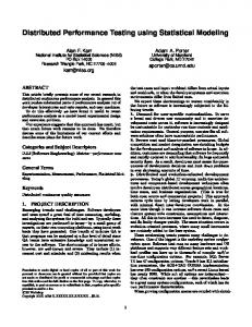
to cope with the high volumes of workload. In this case study, we use our simulation model to evaluate the performance benefits of migrating a centralized performance monitor for ULS systems to a distributed architecture. Since the performance of distributed systems is highly dependent on the configuration, the performance analyst should first determine which configuration of the distributed system provides the best performance. 1) System Description: Performance monitors are used to detect problems in the services provided by a ULS system. Such systems distribute computational units around the world to keep servers geographically close to the users. In the original design, one performance monitor would periodically collect performance data from each computational unit directly. While it is easy to administer, this centralized design has heavy resource requirements. In a distributed design, each computational unit is connected to a local monitoring agent as shown in Figure 6. The local monitoring agents periodically collect, compress and upload the performance data to a central monitor for analysis. The central monitor may occasionally send back an updated set of monitoring policies to the local agents. There are two major challenges involved with monitoring ULS systems: • Communication latency ULS systems are decentralized around the world. Due to the large physical distances between the nodes and the central monitor, the performance data may not reflect the current state by the time the data is received by the central monitor. • Financial cost of data transmission Depending on the frequency with which the performance data is sent, the cost of data transmission may be prohibitively high for ULS systems with many nodes deployed across the globe. 2) Simulation Model: Figure 6 shows the world view layer of the simulation model for the industry-inspired performance monitor used in our case study. The local monitoring agents and the central monitor are modeled using the same architecture as the RSS server (Figure 2). Our simulation model has two tuneable parameters: • Data collection frequency The rate at which local monitoring agents collect performance data from their respective computational units. • Data broadcast period The amount of time an agent would wait between each successive upload of performance data. Data collected by the agents is first stored locally. When the send timer fires, all stored data is uploaded to the central monitor. We conducted a series of simulated runs with 15 combi-

RAM Util. Range (%) Discretization

Low < 25 0.25

OK 25 – 50 0.5

High 50 – 60 0.75

Very High > 60 1

nations of collection frequencies (0.1, 0.2, and 0.3 times per second) and broadcast periods (1, 3, 5, 7, and 9 seconds). Each of the 15 runs simulates an eight-hour workday. Each data collection consumes on average 30 Megabyte of memory and 10 CPU units, and lasts for 3 simulated seconds. Table V shows for each layer the performance data collected during a simulation run. 3) Evaluation of Configurations: In this section, we show that, by considering the performance data from all three layers, we are able to select a configuration that leads to a balance of three important aspects: cost, performance, and resource consumption. For this, we define a score to rank configurations according to multiple performance objectives. Configuration Score We use the concept of configuration score to evaluate a given configuration of performance counters. This score needs to take into account that some counters are perceived by stakeholders in a fuzzy manner. For example, the difference between a CPU utilization of 20% and 25% is hard to observe and hence does not really matter. On the other hand, counters such as the response time and dollar cost are usually perceived by customers in a crisp way. To account for the fuzziness of counter perception, we discretize the fuzzy counter values into discrete levels, where each level is ranked by a number between 0 and 1 according to stakeholder perception. Tables VI and VII show the categorization for CPU and RAM utilizations, respectively. For counters perceived in a crisp way (e.g., response time and cost), we use the original counter values. The configuration score is calculated as the product of the discretized or crisp counter values of a configuration. As a simplified example, if a given configuration exhibits an average response time of 5.61 seconds, consumes on average 46% of the central monitor CPU, and has a cost of $10, then the score of this configuration would be calculated as follows (taking into account the discretization levels of CPU Utilization in Table VI): Responsetime = Cost = CP U U tilization

=

−−−−−−−−− ⇒ Score 7

5.61 seconds $10 46% → 0.5 −−−−−−−−−−

=

5.61 × 10 × 0.5 = 28.1

Fig. 6.

World view layer of the performance monitor for ULS systems.

Figure Error! No text of specified style in document.-1: World view layer of the performance TABLE VIII monitor for ULSDESIGN applications S IMULATION RESULTS FOR THE DISTRIBUTED OF THE PERFORMANCE MONITOR .

! Data Collection Frequency (Hz) 0.1

0.2

0.3

Layers World View Component Physical World View Component Physical World View Component Physical

Data Broadcast Period (s) 1 1 1 1 1 7 1 1 3

Response time (s) 6.8 6.8 6.8 7.7 7.7 8.9 8.9 8.9 9.2

Cost per transmission ($) 5.0 5.0 5.0 5.0 5.0 5.3 5.0 5.0 5.0

Choosing the Optimal Configuration Since we aim to minimize resource consumption, response time and cost, the configuration that has the lowest score gives the best overall performance. Table VIII shows, for each data collection frequency, the three optimal configurations considering the performance data visible up to the designated layer in the second column. For example, we calculate the score of a configuration at the world view layer by multiplying the response time and the cost. If we are to calculate the score at the physical layer level, we would take the product of all five variables (response time, cost, thread, CPU and RAM utilizations). By doing this, we can determine whether early performance modeling by the world view layer stakeholders (Table II) is effective at picking the best configuration. At the lowest data collection frequency (0.1 Hz), the optimal configuration can indeed be determined using the world view layer alone, since it picks the same configuration as the other two layers. This effect is explained by the fact that the system is only slightly loaded and the counters collected in the component and physical layers only exhibit small variations, e.g., RAM utilization ranges between 3% to 6%.

Central Monitor Thread Util. (%) 1.6 1.6 1.6 4.0 4.0 2.3 6.4 6.4 5.6

Central Monitor CPU Util. (%) 15.6 15.6 15.6 40.3 40.3 23.4 64.4 64.4 56.0

Central Monitor RAM Util. (%) 6.1 6.1 6.1 15.7 15.7 9.2 25.3 25.3 21.9

As a result, all low level counters are discretized to the same range, diminishing the effect of these low level counters in the score calculation. Our discretization approach effectively hides the small variations of the performance counter that are insignificant in terms of stakeholder experience. As the data collection frequency increases and more layers are being considered, our ranking algorithm outputs configurations that balance between cost, performance and resource consumption. For example, at the collection frequency of 0.3 Hz, the configuration selected by considering data collected up to the physical layers reduces the CPU utilization from 64.4% to 56% in a tradeoff of 0.3s increase of response time, while maintaining the same cost. In all our experiments, the world view layer performs at least as good as the component layer. 4) Evaluation of the Migration to a Distributed Architecture: Table IX shows the simulation result for the original design of the performance monitor at various data collection frequencies. Comparing to our distributed design (Table VIII), the original design, while providing better response time, consumes more hardware (e.g., CPU and RAM) and logical (e.g., thread) resources. At the collection frequency of 0.3 Hz, 8

TABLE IX S IMULATION RESULTS FOR THE ORIGINAL DESIGN OF THE PERFORMANCE MONITOR . Data Collection Frequency (Hz) 0.1 0.2 0.3

Response time (s) 0.2 0.3 0.4

Cost per transmission ($) 2.2 2.7 3.1

Central Monitor Thread Util. (%) 31.0 43.7 60.2

the CPU of the central monitor is close to running at its full capacity, which will likely result in system instability. Moreover, while the original design has lower cost per transmission, the performance data in the original design is transmitted more frequently due to the absence of a local batching mechanism provided by the local monitoring agent. As a result, the overall cost for monitoring all computational units would increase in the original design compared to the distributed design. In this case study, we demonstrated the usefulness of our layered simulation model in evaluating the different design options for the performance monitor. Furthermore, we show that configurations selected by analyzing information from the top level can provide a good estimation of resource consumption. As more information from different layers is supplied, our ranking algorithm is able to select configurations that balance between cost, performance, and resource consumption.

Central Monitor CPU Util. (%) 42.6 68.2 86.6

Central Monitor RAM Util. (%) 37.2 47.6 59.2

be validated as information becomes available throughout development. Due to the lack of access to production data, we could only estimate a list of resources and processing requirements in our case studies. VII. R ELATED W ORK We discuss four areas of related work: approaches to construct multi-view models, approaches to apply performance modeling at each stage of development, and approaches to create analytical and simulation models. Multi-View Models Kruchten et al. proposed the wellknown “4+1 View” model to describe the different aspects of software architectures [7]. The “4+1 View” model focuses on supporting software architecture understanding for different stakeholders. Our simulation model, on the other hand, focuses on modeling system performance for different stakeholders. Woodside proposed a Three-View Model for performance analysis of concurrent software [20]. The three views in Woodside’s model are drawn from existing analytical techniques and are connected by a “core model” that applies the results of one analytical view to the input of another. Our approach is different from Woodside’s Three-View Model, since our models are based on simulation models and do not require a “core model”. Each layer in the simulation model is built on top of each other, tied together by test case scenarios. Incremental Performance Models Performance modeling can be started at the early stage of software development. Smith et al. proposed a technique to create simple models such as a System Execution Model from usage scenarios with estimates of resource requirements in the beginning of software development [17], [19]. At a later stage, more accurate models such as LQN can be built as more information becomes available. Our model avoids the use of different techniques at different stages in the development, while detailed logic and resource requirements can be added to the simulation model as more information becomes available. Another notable work in this area is the work on run-time performance control (e.g., [25]). Initially, there is no sufficient run-time information available about the software system. Hence, the models used to control the performance of the software system can only use statically available information. Once execution starts, more information becomes available, with which the initial models can be iteratively refined to converge to a more accurate model. Similar to this work, our layered models start out with incomplete information at the world view layer, before being refined based on more accurate lower-layer information.

VI. D ISCUSSION In this section, we discuss how our simulation models can be updated over time and what the major limitations of our approach are. A. Updating the Simulation Model to Reflect System Changes In discrete-event simulations, system components react based on received messages. Therefore, performance analysts can model the system’s behaviour by specifying the state a component should be in when a specific message is received. For example, to simulate the time required to process an RSS notification request, performance analysts can specify that the RSS server would hold each request for 2 simulated seconds before forwarding the notification to subscribers. Performance analysts do not need to know the low-level programming details when constructing the model, which drastically reduces the modeling effort. To update a model constructed for a previous release of a software system to a new version, the resource requirements of the configuration need to be updated. Furthermore, new system behaviour can be introduced into the model by adding new message types and their corresponding behaviour in the simulation code. Once the modified model reflects the new configuration and behaviour, new simulation runs can be performed. B. Capturing Resource Requirements Correct resource requirements are essential in deriving useful performance conclusions from a simulation model. To ensure that the simulation model accurately reflects the performance of the final system, resource requirements should 9

Analytical models The Queuing Network Model (QN) has long been used to analyze the performance of software systems. Baskett et al. proposed algorithms to solve the open, closed, and mixed QN models [1]. Rolia proposed to model complex software systems with layers of servers [13]. Menasc´e proposed an approach to model both the software and hardware resources of a system in a combined model [8]. Woodside et al. proposed an automatic technique to create LQN models from traces of messages passing between software components [22], [6]. However, the quality of the generated layered model depends on the accuracy of the traces. Performance data can be derived from analytical models by solving a set of equations. Because of the use of complex formulas, the knowledge encapsulated in an analytical model can be difficult to transfer to other stakeholders. Furthermore, in order to update analytical models, modelers must possess a certain level of expertise in mathematics. Models built using event-based simulation, on the other hand, can be described using source code, which may provide a lower entrance barrier. Simulation models Smit et al. proposed a simulation framework to support capacity planning for Service-Oriented Architectures (SOA) [16]. Each service in an SOA-based system is modeled as an entity that can send and receive messages. Similar to Smit’s work, our approach can readily be used to model the performance of SOA-based systems. Furthermore, our approach allows modelers to create highly accurate models through the use of layers. Bause et al. extended Petri Nets with Queuing Networks [2]. Xu et al. used coloured Petri Nets to model the architecture of software systems [24]. The authors analyzed performance in time and space based on simulations of test cases. We also simulated test casesto analyze the performance of a software system, however our approach provides modelers with a structured way to construct models suitable for use by multiple stakeholders with varying objectives. Furthermore, by using multiple layers in the simulation model, we effectively create a single, synchronized performance knowledge base that all stakeholders can refer to.

the authors and do not necessarily represent or reflect those of RIM and/or its subsidiaries and affiliates. Moreover, our results do not in any way reflect the quality of RIMs products. R EFERENCES [1] F. Baskett, K. M. Chandy, R. R. Muntz, and F. G. Palacios, “Open, closed, and mixed networks of queues with different classes of customers,” J. ACM, vol. 22, pp. 248–260, April 1975. [2] F. Bause and P. Kemper, “Qpn-tool for qualitative and quantitative analysis of queueing petri nets,” in Proc. of the 7th intl. conf. on Computer performance evaluation, 1994, pp. 321–334. [3] P. C. Clements and L. M. Northrop, “Software architecture: An executive overview,” SEI, Carnegie Mellon, Pittsburgh, PA, USA, Tech. Rep. CMU/SEI-96-TR-003, February 1996. [4] D. Garlan and M. Shaw, “An introduction to software architecture,” SEI, Carnegie Mellon, Pittsburgh, PA, USA, Tech. Rep., 1994. [5] “Google reader,” http://www.google.com/reader/, last access: Jan. 2011. [6] T. A. Israr, D. H. Lau, G. Franks, and M. Woodside, “Automatic generation of layered queuing software performance models from commonly available traces,” in Proc. of the 5th intl. Workshop On Software and Performance (WOSP), 2005, pp. 147–158. [7] P. Kruchten, “The 4+1 view model of architecture,” IEEE Softw., vol. 12, pp. 42–50, November 1995. [8] D. A. Menasc´e, “Two-level iterative queuing modeling of software contention,” in Proc. of the 10th IEEE Intl. Symp. on Modeling, Analysis, and Simulation of Computer and Telecommunications Systems (MASCOTS), 2002, pp. 267–276. [9] D. A. Menasce, L. W. Dowdy, and V. A. F. Almeida, Performance by Design: Computer Capacity Planning By Example. Upper Saddle River, NJ, USA: Prentice Hall PTR, 2004. [10] L. Northrop, Ed., Ultra-Large-Scale Systems – The Software Challenge of the Future. Pittsburgh, PA, USA: SEI, Carnegie Mellon, June 2006. [11] “Omnet++ network simulation framework,” http://www.omnetpp.org/, last access: Jan. 2011. [12] L. F. Pollacia, “A survey of discrete event simulation and state-of-theart discrete event languages,” SIGSIM Simul. Dig., vol. 20, pp. 8–25, September 1989. [13] J. A. Rolia and K. C. Sevcik, “The method of layers,” IEEE Trans. Softw. Eng., vol. 21, pp. 689–700, August 1995. [14] “Rss 0.90 specification,” http://www.rssboard.org/rss-0-9-0/, last access: Jan. 2011. [15] “Rsscloud,” http://rsscloud.org/, last access: Jan. 2011. [16] M. Smit, A. Nisbet, E. Stroulia, A. Edgar, G. Iszlai, and M. Litoiu, “Capacity planning for service-oriented architectures,” in Proc. of the 2008 conf. of the Center for Advanced Studies on collaborative research (CASCON), Toronto, ON, Canada, 2008, pp. 144–156. [17] C. U. Smith and L. G. Williams, Performance solutions: a practical guide to creating responsive, scalable software. Addison Wesley Longman Publishing Co., Inc., 2002. [18] C. U. Smith, Performance Engineering of Software Systems, 1st ed. Boston, MA, USA: Addison-Wesley Longman Publishing Co., Inc., 1990. [19] ——, Encyclopedia of Software Engineering. John Wiley & Sons, January 2002, ch. Software Performance Engineering. [20] C. M. Woodside, “A three-view model for performance engineering of concurrent software,” IEEE Trans. Softw. Eng., vol. 21, pp. 754–767, September 1995. [21] M. Woodside, G. Franks, and D. C. Petriu, “The future of software performance engineering,” in Proc. of the 2007 workshop on the Future of Software Engineering (FoSE), Minneapolis, MN, USA, May 2007, pp. 171–187. [22] M. Woodside, C. Hrishchuk, B. Selic, and S. Bayarov, “Automated performance modeling of softwaree genrated by a design environment,” Perform. Eval., vol. 45, pp. 107–123, July 2001. [23] “Wordpress,” http://wordpress.org/, last access: Jan. 2011. [24] J. Xu and J. Kuusela, “Modeling execution architecture of software system using colored petri nets,” in Proc. of the 1st intl. wrkshp. on Software and performance (WOSP), Santa Fe, NM, USA, 1998, pp. 70– 75. [25] T. Zheng, J. Yang, M. Woodside, M. Litoiu, and G. Iszlai, “Tracking time-varying parameters in software systems with extended kalman filters,” in Proc. of the 2005 Conf. of the Centre for Advanced Studies on Collaborative research (CASCON), 2005, pp. 334–345.

VIII. C ONCLUSION A performance model should convey information about the behaviour of a ULS system relevant to the performance concerns of all stakeholders. Inspired by the “4+1 View” model for software architecture, we proposed an approach to construct simulation models with four layers of abstractions: the world view layer, component layer, physical layer, and usage scenario layer. These layers can be built gradually in a top-down manner as more information about the software project becomes available. Two case studies on complex software systems showed that our layered model can be used to identify performance bottlenecks and evaluate design changes. ACKNOWLEDGMENT We are grateful to Research In Motion (RIM) for providing access to the enterprise application used in our case study. The findings and opinions expressed in this paper are those of 10