Case Study 13 Monitoring Oysters Using Remote Sensing Data and Services: a Case Study of the Apalachicola River and Bay Watershed during Recent Droughts Zhong Liu∗1 and James Acker2
13.1
Background
13.1.1
Study Area: Apalachicola Bay and watershed
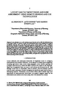
Apalachicola Bay is located on Florida’s northwest coast, consisting of an estuary and lagoon (Figure 13.1a). The Apalachicola River watershed provides the largest inflow of fresh water to the estuary (Figure 13.1b). According to U.S. Geological Survey (USGS) data in 2002, the Apalachicola River, combined with other rivers, drains a watershed of over 20,000 sq. miles (∼52,000 sq. km) at an approximate rate of 19,599 cubic feet per second (∼550 kiloliters per second) of fresh water. Apalachicola Bay is renowned for its oysters, supplying 90% of the oysters in the state of Florida. Major natural threats to the local oyster population are disease, predation and competition from other organisms. Researchers (e.g. Wilber, 1992) found that the balance of Bay water salinity is essential to oyster productivity. Increased salinity can invite marine (salt water) predators to enter the bay from the Gulf. Droughts in the watershed can thus cause less fresh water to flow into the bay and foster a rise in salinity. By contrast, low salinity due to a large fresh water discharge from the river can induce physiological stress to oysters, leading to oyster mortality. Wilber (1992) compared oyster landings for Apalachicola Bay with historical Apalachicola River flows from 1960 – 1984 to determine how river flow and oyster production are related. Since oysters in Apalachicola Bay require 2 years of growth to reach a harvestable size, lag periods were incorporated into the analyses. Wilber (1992) found that low river flows were positively correlated with oyster catch per unit 1 NASA Goddard Earth Sciences Data and Information Services Center; also CSISS, George Mason University, Fairfax, VA, USA. ∗ Email address:
[email protected] 2 NASA Goddard Earth Sciences Data and Information Services Center, Wyle IS LLC, Greenbelt, Maryland, USA
187
188
•
Handbook of Satellite Remote Sensing Image Interpretation: Marine Applications
effort two years later. Wilber’s analyses suggest that sustained high river flows were detrimental to the same year’s harvestable oyster population. Although Wilber’s analyses did not include salinity data, the results imply that a possible mechanism for this association is that lower minimum flows result in higher estuarine salinities, permitting predation by marine species on newly settled spat (juvenile oysters), and thus reducing harvestable oyster population sizes two years later (Wilber, 1992).
Figure 13.1 (a) Apalachicola Bay on Florida’s northwest coast, consisting of an estuary and lagoon; (b) the Apalachicola River watershed (created by "Pfly", based on USGS data, acquired from Wikimedia).
Several other studies have linked oyster growth to freshwater inflows and salinity. Wang et al. (2008) modelled oyster growth rate by coupling oyster population and hydrodynamic models for Apalachicola Bay. Their analyses and model simulations reveal that oyster growth rates were significantly related to salinity. Huang (2010) studied rainfall and river inflow effects on Apalachicola Bay with hydrodynamic modelling and eco-hydrological analysis. During the period 2006 – 2008, historical drought conditions existed in the U.S. Southeast, resulting in severe water shortages. The water shortages were worsened by increasing population, increasing water consumption, and insufficient water conservation measures, which greatly reduced freshwater flow into Apalachicola Bay. Water control for the reservoir Lake Lanier, which provides water for metropolitan Atlanta, made the situation worse. The rising salinity in Apalachicola Bay nearly destroyed the $134 million oyster industry, according to news reports.
13.1.2
Tropical Rainfall Measuring Mission (TRMM)
Drought conditions occur every year around the world. However, monitoring droughts can be a challenging task, especially in data-sparse regions. Satellite remote sensing technology (Maracchi et al., 2000; Liu et al., 2007) provides a unique way to supply precipitation monitoring data from space. In particular, the Tropical Rainfall Measuring Mission (TRMM) – a joint mission between NASA and the Japan Aerospace Exploration Agency (JAXA) – is designed to monitor and study tropical
Monitoring Oysters Using Remote Sensing Data and Services
• 189
and subtropical (40◦ S – 40◦ N) rainfall and latent heat (TRMM Special Issue, 2000). The TRMM satellite flies at an altitude of 402.5 km, and carries three rain-measuring instruments: the TRMM Microwave Imager (TMI), the Visible Infrared Scanner (VIRS), and the Precipitation Radar (PR). TRMM data products are archived and distributed by the Goddard Earth Sciences Data and Information Services Center (GES DISC).
13.1.3
Giovanni TOVAS (TRMM Online Visualization and Analysis System)
Accessing remote sensing products can be a challenging task for users in many developing countries and for non-experts (Liu et al. 2007). For example, many products require different software and computer platforms for processing and visualization, which could require a significant investment from the user side (Liu et al. 2007). To facilitate data access, GES DISC has developed the TRMM Online Visualization and Analysis System (TOVAS), as a part of the "Goddard Interactive Online Visualization ANd aNalysis Infrastructure" or "Giovanni" (Acker and Leptoukh, 2007; Liu et al. 2007; Berrick et al. 2009). With a Web browser and few mouse clicks, an individual can easily obtain global Earth science data visualizations and analyses. The principle design goal for Giovanni was to provide a quick and simple interactive means for scientific data users to study various phenomena by trying various combinations of parameters measured by different instruments, arrive at a conclusion, and then generate graphs suitable for a report or publication. Alternatively, Giovanni can provide a means to ask relevant "what-if" questions and receive rapid results that would stimulate further investigations. These procedures can all be done without having to download and pre-process large amounts of data. A secondary design goal was for Giovanni to be easily configurable, extensible, and portable. GES DISC currently runs Giovanni on Linux, SGI, and Sun platforms. Another goal of Giovanni was to off-load as much of the data processing workload as possible onto the machines hosting the data, and thereby reduce data transfers to a minimum. Given the enormous amount of data at GES DISC in Hierarchical Data Format (HDF), it was a requirement that Giovanni support HDF, HDFEOS, as well as binary data. Giovanni consists of HTML and CGI scripts written in Perl, Grid Analysis and Display System (GrADS http://grads.iges.org/grads/) scripts, and one or more GrADS Data Servers (GDS) running on remote machines that have GrADS readable data. In addition, an image map Java applet can be used to select a bounding box area to process. GrADS was chosen for its widespread use in providing easy access, manipulation, and visualization of Earth science data. It supports a variety of data formats such as binary, GRIB, NetCDF, HDF, and HDFEOS. When combined with the Open-source Project for a Network Data Access Protocol (OPeNDAP), as in GDS, the result is a secure data server that provides subsetting and analysis across the network or even the Internet. The ability of GDS to subset data on the server drastically reduces
190
•
Handbook of Satellite Remote Sensing Image Interpretation: Marine Applications
the amount of data that needs to be transferred across the network, and improves overall performance. GDS provides spatial or temporal subsetting of data while applying any of a number of analysis operations including basic math function, averages, smoothing, correlation, and regression. An equally important feature is the ability to run GrADS data transformations on the server. This case study will demonstrate the use of remote sensing rainfall data products from TRMM (and other sources), combined with data analysis services, to monitor freshwater inflows and salinity that affect oysters in Apalachicola Bay. This study should enhance our ability to understand the dynamics of the Apalachicola Bay estuarine ecosystem, based on the relationships established in previous studies.
13.2
Materials and Methods
13.2.1
Tropical Rainfall Measuring Mission (TRMM) data products
TRMM standard products are available at three levels. Level 1 products are the VIRS calibrated radiances, the TMI brightness temperatures, and the PR return power and reflectivity measurements. Level 2 products are derived geophysical parameters (such as rain rate) at the same resolution and location as those of the Level 1 source data. Level 3 products are the time-averaged parameters mapped onto a uniform space-time grid. An evaluation of the sensor, algorithm performance and first major TRMM results appear in the Special Issue on the Tropical Rainfall Measuring Mission (see Section 13.6.1, Further Reading). Observations from a single satellite usually suffer from limited spatial and temporal coverage. Multi-satellite data can provide wider spatial coverage and often more frequent measurements than a single satellite, making monitoring global environmental conditions a reality. Combined with other satellites (e.g. geostationary satellites and other microwave instruments), TRMM products can be greatly improved in terms of their spatial coverage and temporal resolution (Huffman et al. 2007), such as a 3-hourly TRMM multi-satellite precipitation analysis. Because the TRMM satellite was launched in 1997, its data products can only provide limited historical records. To investigate longer periods, it is necessary to use other products, such as the Global Precipitation Climatology Project (GPCP) monthly precipitation product. GPCP provides a global merged rainfall analysis for research and applications. Data from over 6,000 rain gauge stations, satellite geostationary, and low-orbit infrared, passive microwave, and sounding observations have been merged to estimate monthly rainfall on a 2.5-degree global grid from 1979 to present (http://www.gewex.org/gpcp.html). In this case study, we will use:
v Monthly 0.25◦ x 0.25◦ merged TRMM and other sources estimates (3B43); v the Monthly GPCP 2.5◦ x 2.5◦ merged product.
Monitoring Oysters Using Remote Sensing Data and Services
13.2.2
• 191
USGS streamflow data
To evaluate rainfall impact on fresh water discharge, we use streamflow measurements reported by the USGS (http://waterdata.usgs.gov/nwis/rt) for station 02359170 near Sumatra, FL, in the Apalachicola-Chattahoochee-Flint (ACF) River Basin (Lat 29◦ 56’57", Lon 85◦ 00’56" ). This station measures streamflow from a drainage area of approximately 19,200 mi2 and provides records from September 1977 to the current year. The streamflow data can be downloaded from http://waterdata.usgs.gov/nwis/uv?02359170.
13.2.3
Giovanni TOVAS
Via the TOVAS Web interface, the user selects one or more precipitation data sets, the spatial area, the temporal extent, and the type of output. The selection criteria are passed to the CGI scripts for processing.
13.3
Demonstration
13.3.1
Drought Analysis
With TOVAS, users can investigate the spatial and temporal distribution of the precipitation in their area of interest as well as its climatology and anomalies. Examples are given as follows: 13.3.1.1
Rainfall climatology
Before analyzing drought conditions, it is necessary to understand the rainfall climatology and inter-seasonal, annual variability in the Apalachicola River watershed. First, we will generate a latitude-longitude map and a time series plot, using a web browser to perform the following steps: STEP 1: Visit, http://gdata1.sci.gsfc.nasa.gov/daac-bin/G3/gui.cgi?instance_ id=TRMM_Monthly
STEP 2: Select an area of interest. In this case, we selected a region that includes the Apalachicola river watershed (Figure 13.2a) STEP 3: Select "Climatology" from Analysis Options and "Rain Rate" from the TRMM 3B43 V6 pull-down menu. STEP 4: Select Jan (January) as Begin Date and Dec (December) as End Date in the Temporal selection menu. STEP 5: Click "Generate Visualization". Figure 13.2b is the 12-month climatology (average rain rate) for the region (it may look slightly different based on the area
192
•
Handbook of Satellite Remote Sensing Image Interpretation: Marine Applications
( b) ( a)
( c)
Figure 13.2 (a) TOVAS website showing the area of interest including the Apalachicola watershed; (b) 12-month (Jan – Dec) climatology rain rate (mm h−1 ) for the region; (c) area-averaged time series rain rate climatology.
selected). To plot a time series, repeat the first 3 steps above, except type in the watershed region (Latitudes: 30◦ – 35◦ N; Longitudes: 83◦ – 86◦ W). Select "Time series" from the "Select Visualization" menu and click "Generate Visualization". The plot is shown in Figure 13.2c. Repeat the above steps for different seasons (Dec-Feb, Mar-May, Jun-Aug, SepNov) to obtain the climatology maps showing seasonal changes in rainfall spatial distribution (Figure 13.3). In winter (Dec – Feb) and spring (Mar – May), the highest rain intensity concentrates in the NE watershed and decreases toward the SE. In summer (Jun – Aug) and fall (Sep – Nov), the intensity gradient is reversed with highs in the southern part of the watershed (possibly related to tropical weather systems) along the coastal areas, and lows in the central and northern parts.
13.3.1.2
Obtaining time series and anomaly map in the watershed region
Using the latitudes and longitudes of the watershed, we next plot a 12-year time series of rainfall intensity. The steps are as follows: STEP 1: Go to http://gdata1.sci.gsfc.nasa.gov/daac-bin/G3/gui.cgi?instance_ id=TRMM_Monthly.
Monitoring Oysters Using Remote Sensing Data and Services
• 193
Figure 13.3 Climatology maps showing seasonal changes in the spatial distribution of rainfall (mm h−1 ) for the Apalachicola watershed.
STEP 2: Select a region of interest. Type: Latitudes: 30 – 35◦ N; Longitudes: 83 – 86◦ W and click on "Update Map". STEP 3: Select "Parameter" from Analysis Options and "Rain Rate" from the TRMM 3B43 V6 pull-down menu. STEP 4: Select "Jan 1998" as Begin Date and "Feb 2010" as End Date in the Temporal selection menu. STEP 5: Click "Generate Visualization". Figure 13.4a is the 12-year time series of the average rain rate for the selected region. Select "Anomaly" from the Analysis Options and repeat the above steps, which will obtain the anomaly time series plot (Figure 13.4b). To understand the spatial distribution of the anomaly, we next select two different periods: wetter years between 2003 and 2005 and drier years between 2005 and 2008, by repeating the above steps. Choose "Lat-Lon Map, time-averaged" from the Select Visualization menu to create the figures. The results are shown in Figure 13.5.
194
•
Handbook of Satellite Remote Sensing Image Interpretation: Marine Applications
Figure 13.4 (a) 12-year time series of average rain rate in the Apalachicola watershed; (b) anomaly time series plot for the same region and time frame.
13.3.1.3
Monitor droughts and floods
With TOVAS, users can monitor drought and flood development. Using the Monthly Rainfall (3B43) Anomaly Tool (http://disc2.nascom.nasa.gov/Giovanni/tovas/rain. 3B43_V6_anom.shtml), users can generate the latest monthly rainfall, anomaly and normalized anomaly (normalized anomaly is defined as (rainfall - climatology) / climatology). For example, Figure 13.6a shows the total rainfall in mm for February of 2010, Figure 13.6b shows the corresponding anomaly while Figure 13.6c shows the normalized anomaly in percentage. It can be seen that rainfall is highly nonuniform, with high rainfall being recorded in the Gulf of Mexico (Figure 13.6a). The Apalachicola watershed area also received more rainfall than the surrounding areas (about 20% more than normal). TOVAS also provides near-real-time monitoring services (http://disc2.nascom.
Monitoring Oysters Using Remote Sensing Data and Services
• 195
Figure 13.5 Spatial distribution of the rain rate anomaly (mm h−1 ) in the Apalachicola watershed over wetter years (2003 – 2005) and drier years (2005 – 2008).
nasa.gov/Giovanni/tovas/) with only a few hours data latency. Users can examine
rainfall conditions through TOVAS, which is very useful in monitoring floods. Using TOVAS, users can plot rainfall maps including accumulated rainfall and time series in the area and time period of interest. 13.3.1.4
Further analysis
Users can conduct other analyses by using additional functions (e.g. Hovmöller diagrams, animations, exporting data in ASCII for customized analysis), or other rainfall products (e.g. 3-hourly, daily, 10-day). The following steps show how to download rainfall data in ASCII and import them in Microsoft Excel for further analysis. STEP 1: Follow Section 13.3.1.2 and generate a time series for the period of interest. STEP 2: Click "Download Data" STEP 3: Click the ASCII thumbnail in "Download Files" to display the ASCII output data. STEP 4: From your browser menu, click Edit and select "Select All". The data will be highlighted. Select "Copy" and paste them in a Microsoft Excel spreadsheet. STEP 5: Highlight the data column and select "Data" and "Text to Columns". The action will split the pasted data into two columns.
196
•
Handbook of Satellite Remote Sensing Image Interpretation: Marine Applications
Figure 13.6 (a) Total rainfall (mm) for February of 2010; (b) rainfall anomaly (mm) for February 2010; (c) normalized rainfall anomaly (%).
STEP 6: Plot the data and add a trend line (Figure 13.7). The files can be downloaded from: http://disc.sci.gsfc.nasa.gov/giovanni/precipitation_case_study_files/
13.3.2 13.3.2.1
Impact Analysis USGS streamflow discharge
As mentioned in the Introduction, freshwater discharge has important impacts on Apalachicola Bay ecological systems. Users can obtain real-time and historical streamflow data for the Apalachicola Bay from the U.S. Geological Survey web site (http://waterdata.usgs.gov/nwis/rt). To demonstrate rainfall and its impact on streamflow, we use the monthly data. Below are the steps to obtain monthly streamflow time series: STEP 1: Go to http://waterdata.usgs.gov/nwis/uv?02359170 STEP 2: Select Time-series: Monthly statistics from Available data for this site. Click "Go" STEP 3: Select Parameter Code 00060. Select Tab-separated data. Select Display in browser. Click Submit. STEP 4: In your web browser, click Edit, Select All and Copy, then paste into an Excel
Monitoring Oysters Using Remote Sensing Data and Services
• 197
Figure 13.7 Time-series of rain rate (mm h−1 ) plotted with MS Excel©, with a trendline added to the time-series data plot.
Spreadsheet. Since the GPCP rainfall product provides a longer period of monitoring, we demonstrate how to plot it against the USGS streamflow discharge data described above. The results are shown in Figure 13.8. In general, rainfall in the Apalachicola watershed region has a close tie to the streamflow discharge data measured near the bay at Sumatra, FL, although the discharge can be controlled by many factors including upstream water storage and withdrawals. 13.3.2.2
Salinity analysis
Salinity data downloaded from the National Data Buoy Center and imported into Microsoft Excel can be plotted along with the rainfall data for comparison. Figure 13.9a shows the time series of the rain rate averaged over the watershed region, and the salinity measured in the Apalachicola Bay. Note that when salinity rises, the rain rate is low and vice versa over the 30-month period. Similarly, we can plot the USGS streamflow discharge data along with the salinity data. Figure 13.9b shows that when streamflow discharge is high, salinity is low and vice versa. These two figures illustrate the impact of rainfall and streamflow discharge on salinity in Apalachicola Bay.
13.4
Training and Questions
Q1: Why are the data presented in mm/hr? How can I convert mm/hr in TRMM 3B43 to mm/month? Q2: Describe the spatial distribution of rainfall in the watershed region. Is it uniform? When do the rainfall maxima in the study region occur for average conditions? Q3: Is the spatial distribution of rainfall consistently the same for different seasons?
198
•
Handbook of Satellite Remote Sensing Image Interpretation: Marine Applications
Figure 13.8 The GPCP (Global Precipitation Climatology Project) monthly rainfall product (blue line) and the USGS streamflow discharge (red line) for Apalachicola Bay, from January 1979 to November 2007.
Q4: 4. In Figure 13.4a, attempt to identify months and periods with unusually high and unusually low rainfall. Then look at the anomaly time-series (Figure 13.4b). Are the periods you identified consistent with the rainfall anomalies? What were the main periods of below-average rainfall, according to Figure 13.4b? Q5: 5. Is the spatial distribution of rainfall during dry years and wet years the same, or different? What meteorological phenomena might explain these observations? Q6: Was rainfall in February 2010 in the watershed region above normal, approximately normal, or below normal, based on the climatological average? (Figure 13.6)
Monitoring Oysters Using Remote Sensing Data and Services
• 199
Figure 13.9 (a) Time series of rainfall rate (mm h−1 ) averaged over the Apalachicola watershed region (blue line), and the salinity (psu) measured in the Apalachicola Bay (red line); (b) USGS streamflow discharge data (cubic feet per second, green line) along with the salinity data (red line).
200
•
Handbook of Satellite Remote Sensing Image Interpretation: Marine Applications
Q7: 7. Based on Figure 13.8, is there a strong correlation, a weak correlation, or no correlation between the GPCP monthly rainfall values and the USGS streamflow discharge data? Does your conclusion surprise you? Q8: Is there a positive correlation, a negative correlation, or no correlation between precipitation in the watershed and salinity in Apalachicola Bay as measured by the NOAA buoy (Figure 13.9a)? Q9: Is there a positive, negative, or no correlation between streamflow in the watershed and salinity in Apalachicola Bay as measured by the NOAA buoy (Figure 13.9b)? Q10: In light of the background information provided about the Apalachicola Bay oyster fishery, what recommendations could be made based on these observations regarding preservation of the fishery in relation to precipitation and streamflow in the watershed?
13.5
Answers
A1: Because the total number of days in each month are different, mm/hr is used for easy comparison. Since the 3B43 product is a monthly average, you could simply do the conversion by multiplying the hourly rain rate by the total number of hours in that month. A2: From Figure 13.2b, it is seen that the spatial distribution of rainfall is not uniform in the watershed region. The rain intensity decreases from west to east with highs in the northern and southern ends of the region. The time series plot shows that there are two rain maxima, one in March and the other in July. May and November are the two months with minimum rainfall. A3: 3. Figure 13.3 shows that seasonal changes in rainfall spatial distribution are different. In winter and spring, the highest rain intensity concentrates in the NE watershed and decreases toward the SE. In summer and fall, the intensity gradient is reversed with highs in the southern part of the watershed (possibly related to tropical weather systems) along the coastal areas, and lows in the central and northern parts. A4: 4. From the time series of the past 12 years (Figure 13.4 a,b), it can be seen that the monthly rainfall intensity is highly variable. Between 1998 and 2003, the region experienced below normal rainfall intensity, and an above average rainfall intensity after that period. The region experienced another below average rainfall intensity from mid-2005 to -2008, but this dry spell has improved since 2009, with aboveaverage rainfall. The time series also shows that the latest dry period (mid-2005 to
Monitoring Oysters Using Remote Sensing Data and Services
• 201
-2008) was the worst in this 12-year record. The region experienced more than 3 consecutive years of below-normal rainfall. A5: Figure 13.5 shows that the spatial distributions of the anomaly between the wetter and drier than normal years are quite different. In the wetter years, more rain fell in the central and the northern parts of the region; in contrast, during the drier years, considerably less rain fell in the northern region. During dry years, one of the notable contributions to rainfall are storm systems in the Gulf of Mexico (either winter lows or tropical systems), which tend to bring more rain to the coast than inland. A6: Rainfall in February 2010 was below normal, as demonstrated by both the rainfall anomaly, and normalized rainfall anomaly having negative values in the watershed region. The normalized rainfall anomaly indicates that rainfall in February 2010 was only slightly below normal. A7: Figure 13.8 shows that during many periods of high precipitation, there is a strong correlation between high precipitation and high discharge. This is likely due to high discharge rates caused by a large contribution of runoff to streams in the watershed. However, during periods of average or low precipitation, the correlation is considerably weaker. This could be due to natural storage (i.e. replenishment of groundwater, filling of wetlands, increased soil moisture) as well as streamflow control by artificial impoundments, particularly reservoir lakes. A8: There is a negative correlation between precipitation in the watershed and salinity in Apalachicola Bay. This indicates that high precipitation leads to reduced salinity in the Bay, and low precipitation leads to increased salinity in the Bay. A9: There is an apparent negative correlation between streamflow (discharge) in the watershed and salinity in Apalachicola Bay. This indicates that elevated streamflow, which is related to increased precipitation, causes reduced salinity in the Bay, and that reduced streamflow (likely due to both drought and some degree of human control) causes increased salinity in the Bay. A10: 10. Based on all of these observations, it appears that Apalachicola Bay should be guaranteed a minimum flow of freshwater to provide suitable survival conditions for the oyster industry. Obviously, the economic value of the oyster fishery must be balanced against other societal concerns, but it would likely take several years to recover from a significant degradation of the oyster fishery, under normal rainfall conditions.
13.6
References
Acker J G and Leptoukh G (2007). Online analysis enhances use of NASA earth science data. Eos Trans Amer Geophys Union, 88 (2), 14-17
202
•
Handbook of Satellite Remote Sensing Image Interpretation: Marine Applications
Berrick SW, Leptoukh G, Farley JD, and Rui H (2009) Giovanni: A Web service workflow-based data visualization and analysis system. IEEE Trans Geosci Remote Sens, 47 (1), 106-113 Huang W (2010) Hydrodynamic modeling and ecohydrological analysis of river inflow effects on Apalachicola Bay, Florida, USA, Estuarine, Coastal and Shelf Science, Volume 86, Issue 3, 10 February 2010, Pages 526-534 Huffman GJ, Adler RF, Bolvin DT, Gu G, Nelkin EJ, Bowman KP, Hong Y, Stocker EF, Wolff DB, (2007), The TRMM Multi-satellite Precipitation Analysis: Quasi-Global, Multi-Year, Combined-Sensor Precipitation Estimates at Fine Scale J Hydrometeor, 8(1), 38-55 Liu Z, Rui H, Teng W, Chiu L, Leptoukh G, and Vicente G (2007), Online visualization and analysis: A new avenue to use satellite data for weather, climate and interdisciplinary research and applications. Measuring Precipitation from Space - EURAINSAT and the future, Advances in Global Change Research, 28, 549-558 Wilber D (1992) Associations between freshwater inflows and oyster productivity in Apalachicola Bay, Florida. Estuarine, Coastal and Shelf Science, Volume 35, Issue 2, 179-190 Wang H, Huang W, Harwell MA, Edmiston L, Johnson E, Hsieh P, Milla K, Christensen J, Stewart J and Liu X (2008), Modeling oyster growth rate by coupling oyster population and hydrodynamic models for Apalachicola Bay, Florida, USA , Ecological Modelling, Volume 211, Issues 1-2, 24 February 2008, Pages 77-89
13.6.1
Further Reading
Special Issue on the Tropical Rainfall Measuring Mission (TRMM) (2000) – a combined publication including: v The December 2000 issue of the Journal of Climate v Part 1 of the December 2000 Journal of Applied Meteorology (American Meteorological Society, Boston, MA)
13.7
Supplemental Information
What are the other commonly-used TRMM data products? The GES DISC also archives 3-hourly and daily rainfall products for analysis. Details are found in http://disc2.nascom.nasa.gov/Giovanni/tovas/ or http://mirador. gsfc.nasa.gov/cgi-bin/mirador/presentNavigation.pl?tree=project&project=TRMM.
Where can I find more information on the TRMM Data Set? More information on the TRMM instruments and science can be found at the GES DISC TRMM Data Web site: http://disc.sci.gsfc.nasa.gov/precipitation/ How current are the TRMM data? The GES DISC receives, under normal circumstances, processed standard orbital/swath data products about 2-3 days after satellite data acquisition, depending on the level of processing required. In addition to this ongoing collection of data, archives of older data are maintained. What is the GES DISC Search and Order Web Interface?
Monitoring Oysters Using Remote Sensing Data and Services
• 203
The GES DISC data search and order interface is a simple point-and-click web interface that is based on a hierarchical organization of data, displayed as tables. At different levels of the hierarchy, the tables contain some or all of the following: a particular data product grouping such as data product name, year, or month in the first column on the left; followed by columns of short description, begin date, end date, number of items available in the archives, average item size, a preview feature (if a data product has browse images), and documentation ("readme"). The last column on the right allows one to "Select" an item. At certain levels of the hierarchy, you can also use orbital and parameter search features to customize your search. Specific help is provided at the top of each page of this system (http://disc.sci.gsfc.nasa.gov/data/datapool/TRMM/index.html). Where can I find some documentation describing TRMM and TRMM data? Information about TRMM and TRMM data can be found in:
v TRMM related documentation, describing the science, the instruments, data processing, and data access. v TRMM "ReadMe" and "Data Access" documents on the data products and direct data access. v Precipitation Processing System/TRMM Science Data and Information System (PPS/TSDIS) documentation, providing the details of all the products. v Tutorial for "Reading TRMM Data Products" Where can I find information describing the TRMM algorithms? Information about algorithms used for the TRMM products can be found in the Algorithm Status Page, where the links to the products take you to brief descriptions of the status of the products and, for some products, key references. How are the daily products computed from 3B42RT and Version 6 3B42 in TOVAS? These daily products are computed by averaging all the estimates available in the eight observation times of a given UTC day, namely 00, 03, ..., 21 UTC. Formally, this "day" covers the period from 2230 UTC of the previous day through 2230 UTC of the given day. Other "day" products can be computed interactively for 3B42RT and Version 6 3B42 by specifying similar 8-period runs of data. For example, a day that starts at 09 UTC can be approximated by taking data from 09 UTC of one day through 06 UTC of the next. At present, there is no capability in TOVAS for a more exact approximation of a "day" for these data sets. What is the key documentation describing the 3B42RT and Version 6 3B42 products? The paper by Huffman et al. (2007) describing the 3B42RT (real-time) and Version 6
204
•
Handbook of Satellite Remote Sensing Image Interpretation: Marine Applications
3B42 (research quality) products of the TRMM Multi-satellite Precipitation Analysis (TMPA) is accessible at ftp://meso.gsfc.nasa.gov/agnes/huffman/papers/TMPA_ jhm_07.pdf.gz Technical documentation is also available for the research product and real-time product, as is a WHATSNEW file, which contains recent notices about issues with the RT product. What is the difference between the real time and research products of the TRMM Multi-satellite Precipitation Analysis (TMPA)? Version 6 research products are the "real" TRMM products. They are produced monthly, and are available 2-3 weeks after the end of the month. The upgrade to Version 6 happened in Spring/Summer 2005. Reprocessing evaluations for the next version of the data (Version 7) are currently being performed. Version 7 will constitute a reprocessing of the entire record from January 2008 to the present time. Institutionally, TRMM has been joined by a successor project, Global Precipitation Measurement (GPM), which has a nominal launch date of 2013. In the GPM era, a combination-product successor to the TMPA is a high priority, so there is a strong likelihood for a long time series of a consistent data product (via episodic reprocessing). The real-time (RT) products are experimental products posted due to the high demand for such information. RT products are not reprocessed (except for processing failures). A major upgrade occurred in February 2005, so the processing scheme since then has been relatively consistent. The latest upgrade in February 2010 attempted to make the RT relatively consistent with Version 6 research products. For continuity, however, the data files will also include a precipitation field that is "more or less" the old RT result. Whenever possible, users are urged to take advantage of the improved quality of the research products. Some operational applications, however, cannot wait for the research products, and the RT products are intended for those application users. What are the caveats in using TRMM Multi-satellite Precipitation Analysis (TMPA) products? The following are some caveats in using TMPA:
v The key caveat is that all of the TMPA products are research products, not "operational" (i.e. no contingency plans or backup system in case of a network failure or a disk crash). v The TMPA is a gridded product, which is different from the point rain gauge data that might be more familiar to users, but grid values are more appropriate for certain applications. v Although the TMPA analysis scheme is consistent for the time period of a given version, the suite of input data varies. For example, there is less of the (higher-quality) microwave data before 2001; the infrared data are on a coarser
Monitoring Oysters Using Remote Sensing Data and Services
v
v
v v
• 205
grid in 1998 – 1999; gauge sites report individually, and are therefore subject to availability issues, particularly in developing countries. Occurrence of precipitation over land tends to be underestimated because satellite schemes tend to miss light precipitation and precipitation that is enhanced by flow lifting over mountains. Occurrence and amount of precipitation in some, but not all, coastal areas tends to be underestimated. Conversely, arid coastal areas (oceans and lakes) sometimes show persistent artefacts. Both effects are due to issues in the input microwave estimates. The RT amounts tend to be biased high in warm-season convective weather due to biases in the input microwave estimates. The Version 6 data tend to be biased low in regions of complex terrain due to gauge-location biases toward lower elevations.