Multi-Colony Ant Algorithms for the Dynamic Travelling ... - IEEE Xplore

Multi-Colony Ant Algorithms for the Dynamic Travelling Salesman Problem Michalis Mavrovouniotis and Shengxiang Yang

Xin Yao

Centre for Computational Intelligence (CCI) School of Computer Science and Informatics De Montfort University The Gateway, Leicester, LE1 9BH, UK Email: {mmavrovouniotis, syang}@dmu.ac.uk

CERCIA School of Computer Science University of Birmingham Birmingham B15 2TT, UK Email: [email protected]

Abstract—A multi-colony ant colony optimization (ACO) algorithm consists of several colonies of ants. Each colony uses a separate pheromone table in an attempt to maximize the search area explored. Over the years, multi-colony ACO algorithms have been successfully applied on different optimization problems with stationary environments. In this paper, we investigate their performance in dynamic environments. Two types of algorithms are proposed: homogeneous and heterogeneous approaches, where colonies share the same properties and colonies have their own (different) properties, respectively. Experimental results on the dynamic travelling salesman problem show that multi-colony ACO algorithms have promising performance in dynamic environments when compared with single colony ACO algorithms.

I.

I NTRODUCTION

Ant colony optimization (ACO) algorithms are inspired from nature, i.e., the foraging behaviour of real ant colonies [3], [7]. Most of the optimization problems addressed so far by ACO assume a stationary environment. However, the environment in many real-world applications changes over time. The difference between stationary and dynamic optimization problems (DOPs) is that the aim for the former type of problems is to locate the static global optimum efficiently whereas the aim for the latter type of problems is to track the moving global optimum efficiently [12], [23], [30]. Addressing DOPs is challenging to ACO algorithms, and generally to all optimization algorithms. Once an ACO algorithm converges to an optimum, then it is difficult for the algorithm to escape from it in order to track the newly generated optimum when a dynamic change occurs. The pheromone trails, generated with ACO algorithms, of the previous environment may bias the colony1 of ants towards the optimum of the previous environment. A direct way to address this issue is to consider every dynamic change as the arrival of a new problem instance that needs to be solved from scratch by re-initializing all the pheromone trails with an equal amount. However, such strategy may be computationally expensive and requires the detection of a dynamic change. In case the changing environments have similarities, the re-optimization time may be improved by transferring knowledge from previous environments [1], [12], [15], [23]. 1A

term used in ACO, which also denotes a population.

978-1-4799-4515-3/14/$31.00 ©2014 IEEE

Over the years, several strategies have been proposed to enhance the performance of ACO algorithms for DOPs, including increasing diversity after a change [8], [10], maintaining diversity during the execution [15], [16], memory-based schemes [11] and memetic algorithms [14]. Although multipopulation approaches have shown promising performance for evolutionary algorithms [5] and particle swarm optimization [2] when addressing DOPs, they have attracted little (or no) attention for ACO. Hence, in this paper we attempt to apply multi-colony ACO algorithms in dynamic environments and investigate their performance. In this paper, the investigated multi-colony ACO algorithms consist of more than one colony, where each colony has its own pheromone table and exchange information occasionally. In this way, the search area explored is increased. If the colonies have the same searching behaviour, they are called homogeneous; otherwise, if the colonies have different searching behaviour, they are called heterogeneous. Based on the dynamic benchmark generator proposed in [17], a series of dynamic test cases are constructed from several stationary travelling salesman problem (TSP) benchmark instances and experiments are systematically carried out for single and multicolony ACO algorithms. The rest of the paper is organized as follows. Section II describes the dynamic TSP (DTSP) generated by the benchmark generator. Sections III and IV describe the traditional single colony ACO and proposed multi-colony ACO, respectively. Section V gives the experimental results of ACO algorithms regarding their overall performance in dynamic environments. Finally, Section VI concludes this paper and outlines several future works. II.

DYNAMIC T RAVELLING S ALESMAN P ROBLEM

The TSP can be described as follows: given a collection of cities, the objective is to find the Hamiltonian cycle that starts from one city and visits each of the other cities once before returning to the starting city. Typically, the problem is modelled by a fully connected weighted graph 𝐺 = (𝑁, 𝐴), where 𝑁 = {0, . . . , 𝑛} is a set of nodes and 𝐴 = {(𝑖, 𝑗) : 𝑖 ∕= 𝑗} is a set of arcs. Each arc (𝑖, 𝑗) is associated with a non-negative value 𝑑𝑖𝑗 which represents the distance between cities 𝑖 and 𝑗.

Formally, the TSP is defined as follows. Let 𝜓𝑖𝑗 denote the binary decision variables defined as follows: { 1, if (𝑖, 𝑗) is covered in the tour, (1) 𝜓𝑖𝑗 = 0, otherwise, where 𝜓𝑖𝑗 ∈ {0, 1}. Then, the objective of the TSP is defined as follows: 𝑛 ∑ 𝑛 ∑ 𝑓 (𝑥) = 𝑚𝑖𝑛 𝑑𝑖𝑗 𝜓𝑖𝑗 , (2) 𝑖=0 𝑗=0

where 𝑛 is the number of cities and 𝑑𝑖𝑗 is the distance between cities 𝑖 and 𝑗. A. Dynamic Benchmark Generators Over the years, several dynamic benchmark generators have been proposed for the TSP that tend to model real-world scenarios, such as the DTSP with traffic factors [8], [16], [18] and the DTSP with exchangeable cities [10], [11]. These benchmark generators modify the fitness landscape, whenever a dynamic change occurs, and cause the optimum value to change. In this paper, the recently proposed dynamic benchmark generator for permutation-encoded problems (DBGP)2 is used [17], which can convert any stationary permutation-encoded benchmark problem instance to a DOP. The fitness landscape is not changed with DBGP, and thus, the optimum value (if known) remains the same. This is because DBGP shifts the population of the algorithm to search to a new location in the fitness landscape. The main advantage of using the DBGP rather than the other generators is that one can observe how close to the optimum an algorithm can perform when a dynamic change occurs. However, DBGP sacrifices the realistic modelling of application problems for the sake of benchmarking. B. Constructing Dynamic Test Environments Considering the TSP description, each city 𝑖 ∈ 𝑁 has a location defined by (𝑥, 𝑦) and each link (𝑖, 𝑗) ∈ 𝐴 is associated with a non-negative distance 𝑑𝑖𝑗 . Usually, the distance matrix of a problem instance is defined as D = (𝑑𝑖𝑗 )𝑛×𝑛 . DBGP generates the dynamic case as follows. ⃗ (𝑇 ) is generated that Every 𝑓 iterations a random vector 𝑉 contains exactly 𝑚 × 𝑛 cities where 𝑇 = ⌈𝑡/𝑓 ⌉ is the index of the period of change, 𝑡 is the iteration count of the algorithm, 𝑓 determines the frequency of change, 𝑛 is the size of the problem instance, and 𝑚 determines the magnitude of change. More precisely, 𝑚 ∈ [0.0, 1.0] defines the degree of change, in ⃗ (𝑇 ) city locations are swapped. which only the first 𝑚×𝑛 of 𝑉 ⃗ (𝑇 ) is generated that Then, a randomly re-ordered vector 𝑈 ⃗ contains only the cities of 𝑉 (𝑇 ). Therefore, exactly 𝑚 × 𝑛 pairwise swaps are performed in D using the two random ⃗ (𝑇 )⊗ 𝑈 ⃗ (𝑇 )), where “⊗” denotes the swap operator. vectors (𝑉 2 Available

from www.tech.dmu.ac.uk/∼mmavrovouniotis/Codes/DBGP.zip.

III.

S INGLE C OLONY A NT A LGORITHMS

A. ℳ𝒜𝒳 -ℳℐ𝒩 Ant System (ℳℳAS) Algorithm Within ACO a colony of 𝜇 ants constructs solutions and updates pheromone. In this paper, we consider one of the state-of-the-art ACO variations, i.e., ℳ𝒜𝒳 -ℳℐ𝒩 Ant System (ℳℳAS) [25], [26]. Considering the application of TSP described in Section II, all ants are placed on a randomly selected city and all pheromone trails are initialized with an equal amount of pheromone. All ants choose the next city based on existing pheromone trails and some heuristic information using a probabilistic decision rule. With probability 1 − 𝑞0 , where 0 ≤ 𝑞0 ≤ 1, the 𝑘-th ant, when being located at city 𝑖, selects the next city 𝑗 probabilistically, which is defined as follows: 𝑝𝑘𝑖𝑗 = ∑

𝛼

[𝜏𝑖𝑗 ] [𝜂𝑖𝑗 ] 𝑙∈𝑁𝑖𝑘

𝛽

𝛼

[𝜏𝑖𝑙 ] [𝜂𝑖𝑙 ]

𝛽

, if 𝑗 ∈ 𝑁𝑖𝑘 ,

(3)

where 𝜏𝑖𝑗 and 𝜂𝑖𝑗 are the existing pheromone trail and heuristic information, respectively, between cities 𝑖 and 𝑗. The available heuristic information is defined as the inverse of distance, i.e., 𝜂𝑖𝑗 = 1/𝑑𝑖𝑗 . 𝑁𝑖𝑘 denotes the neighbourhood of unvisited cities of ant 𝑘 when its current city is 𝑖. 𝛼 and 𝛽 are the two parameters that determine the relative influence of pheromone trail and heuristic information, respectively. Otherwise, with probability 𝛼 𝛽 𝑞0 , ant 𝑘 selects the city with the highest [𝜏𝑖𝑗 ] [𝜂𝑖𝑗 ] . Right after all ants construct their solutions, they proceed with the pheromone update. The amount of pheromone is tuned according to their solution quality. For example, the better the solution quality, the more the pheromone will be deposited. However, before adding any pheromone, a constant amount of pheromone is deducted from all trails due to the pheromone evaporation, which is defined as: 𝜏𝑖𝑗 ← (1 − 𝜌) 𝜏𝑖𝑗 , ∀ (𝑖, 𝑗),

(4)

where 0 < 𝜌 ≤ 1 is the rate of evaporation. After evaporation, the best ant deposits pheromone to the corresponding trails of their solution as follows: 𝑏𝑒𝑠𝑡 𝜏𝑖𝑗 ← 𝜏𝑖𝑗 + Δ𝜏𝑖𝑗 , ∀(𝑖, 𝑗) ∈ 𝑇 𝑏𝑒𝑠𝑡 ,

(5)

𝑏𝑒𝑠𝑡 = 1/𝐶 𝑏𝑒𝑠𝑡 , 𝑇 𝑏𝑒𝑠𝑡 is the tour of the best ant and where Δ𝜏𝑖𝑗 𝑏𝑒𝑠𝑡 is the solution quality of either the best-so-far ant or the 𝐶 iteration-best ant. Both ants are allowed to deposit pheromone in an alternate way (for more details see [26]).

In ℳℳAS, pheromone trail limits are imposed to [𝜏𝑚𝑖𝑛 , 𝜏𝑚𝑖𝑛 ], where 𝜏𝑚𝑖𝑛 and 𝜏𝑚𝑎𝑥 denote the lower and upper pheromone trail limits, respectively, in order to avoid the stagnation behaviour. The upper pheromone limit is defined by 1/𝜌𝐶 𝑏𝑒𝑠𝑡 where each time a new best-so-far ant is found the 𝜏𝑚𝑎𝑥 value is updated. The lower pheromone trail limit is defined as 𝜏𝑚𝑖𝑛 = 𝜏𝑚𝑎𝑥 /𝑎, where 𝑎 is a pre-defined parameter (for more details see [26]). Finally, the pheromone trails are occasionally re-initialized to 𝜏𝑚𝑎𝑥 whenever the stagnation behaviour occurs. B. Response to Dynamic Changes ACO algorithms can adapt to dynamic changes since they are inspired from nature, which is a continuous changing environment [3], [12]. Practically, they can adapt by transferring

knowledge from past environments via pheromone trails [1], [15]. So far, the description of ACO algorithms given above has been made assuming stationary environments. The diversity within a colony in ACO needs to be enhanced in order to adapt well to environmental changes. Stagnation behaviour eliminates the adaptation capabilities of ACO algorithms. More precisely, when a dynamic change occurs, it is challenging for the colony to escape from the previously converged optimum in order to search for the newly generated one. This is because the high concentration of pheromone trails generated around the old optimum forces the colony to still construct solutions for the previous environment rather than exploring the new one. Pheromone evaporation is important for ACO’s adaptation when addressing DOPs [15]. This is because pheromone evaporation helps to eliminate older pheromone trails. Therefore, when a dynamic change occurs, the colony will be able to escape from the previously converged optimum. IV.

M ULTI -C OLONY A NT A LGORITHMS

Multi-colony ACO algorithms consist of more than one colony of ants that cooperate in order to better explore and exploit the search space, where each colony uses its own pheromone table. In this way, several colonies are able to independently tackle the optimization problem in parallel in an attempt to maximize the search area explored/exploited. Multi-colony ACO algorithms were successfully applied to the vehicle routing problem [9], TSP [22], shortest common supersequence problem [19], [20], and quadratic assignment problem [27]. A comprehensive survey for multi-colony ACO algorithms is available in [24]. Most multi-colony applications consider stationary environments. In this paper, different multi-colony algorithms based on the ℳℳAS development are proposed and applied to the DTSP described in Section II. The multi-colony algorithms may contain colonies that have either different or identical parameter settings, known as heterogeneous and homogeneous, respectively. Different behaviour between ant colonies can be achieved by a different decision rule, objective function, pheromone strategy, and so on. In [18], different 𝑞0 values of the decision rule are used to each colony for the DTSP with traffic factors. For example, the colonies that use 𝑞0 values closer to 0 explore more than colonies that use 𝑞0 values closer to 1. However, this approach is not a pure multi-colony because the different colonies share the same pheromone table. In [9], different objective functions are used to address the vehicle routing problem. For example, one colony is used to minimize the number of vehicles used and another colony is used to minimize the distance travelled by vehicles. Traditional ACO algorithms suffer from the stagnation behaviour, which is mainly caused by the distribution of trails in the pheromone table into a single path. However, the key idea when addressing DOPs is to maintain the diversity of solutions within a colony during the optimization process. By splitting the colony into several colonies that use their own pheromone tables, exploration may be enhanced since different colonies will search and converge into different areas in the search space. Hence, when a dynamic change occurs, the multi-colony approach gains knowledge from a set of

Algorithm 1 Multi-colony ACO framework 1: InitializePheromoneTables 2: while (termination condition not met) do 3: ConstructSolutions 4: end while 5: UpdateBestAnts 6: if (best-so-far ant is found) then 7: Migration 8: end if 9: UpdatePheromone

previously good solutions whereas the single colony approach gains knowledge only from a single solution. The proposed multi-colony ACO algorithms consist of the following main features: ∙

All colonies consist of the same number of ants

∙

All colonies run the same number of iterations

∙

All colonies share the same heuristic information but different pheromone tables

∙

All colonies optimize the same function

∙

The global best solution is migrated to all colonies when a new best-so-far ant is found (an extra pheromone deposit is also performed)

∙

Each colony has its own set of parameters

The complete framework of multi-colony ACO algorithms proposed in this paper is illustrated in Algorithm 1. In this paper, a different evaporation rate 𝜌 is used for each colony in heterogeneous ℳℳAS. In this way, the searching behaviour of colonies differ regarding the adaptation speed. When 𝜌 is set to a small value, slow adaptation is achieved; whereas when 𝜌 is set to a large value, fast adaptation is achieved [15]. V.

E XPERIMENTAL R ESULTS

A. Experimental Setup In the experiments, the performance of two homogeneous multi-colony ACO algorithms against their corresponding single colony ACO algorithms is investigated. Additionally, a heterogeneous multi-colony ACO algorithm is also investigated. All common algorithmic parameters were set as follows: 𝛼 = 1 and 𝛽 = 5. For the single colony ℳℳAS algorithms, the number of ants was set to 𝜇 = 50. The evaporation rate was set to 𝜌 = 0.2 and 𝜌 = 0.8 to indicate a ℳℳAS algorithm with slow and fast adaptation, respectively, marked as ℳℳAS(𝜌). Multi-colony ℳℳAS consists of two colonies, where each colony consists of 50 ants, respectively. The evaporation rate for the homogeneous multi-colony ℳℳAS algorithms was set to 𝜌 = 0.2 and 𝜌 = 0.8, respectively, for both colonies, and for the heterogeneous multi-colony ℳℳAS algorithm was set to 𝜌 = 0.2 and 𝜌 = 0.8 for each colony, respectively. Similar to the single colony algorithms, the multi-colony algorithms are marked as ℳℳAS(𝜌, 𝜌).

TABLE I.

E XPERIMENTAL RESULTS REGARDING THE OFFLINE ERROR OF ACO ALGORITHMS . B OLD VALUES INDICATE THE BEST RESULTS Algorithms & DTSPs 𝑓 = 500, 𝑚 ⇒

kroA100(Optimum=21282)

kroA150(Optimum=26524)

0.1

0.25

0.5

0.75

0.1

0.25

0.5

0.75

0.1

0.25

0.5

0.75

ℳℳAS(0.2)

1254

3502

4524

4777

2783

5377

6510

6755

3975

6836

8028

8256

ℳℳAS(0.8)

1724

3479

4162

4272

3566

5390

5959

6088

5031

6800

7402

7453

ℳℳAS(0.2,0.2)

1673

3446

4539

4903

3426

5385

6644

6999

4502

6837

8109

8523

ℳℳAS(0.8,0.8)

1718

3419

4026

4141

3570

5263

5859

5991

4793

6570

7181

7236

ℳℳAS(0.2,0.8)

1655

3371

4212

4442

3423

5248

6175

6365

4571

6595

7527

7727

𝑓 = 5000, 𝑚 ⇒

0.1

0.25

0.5

0.75

0.1

0.25

0.5

0.75

0.1

0.25

0.5

0.75

ℳℳAS(0.2)

464

943

1304

1495

1128

1962

2423

2513

1176

2243

3100

3211

ℳℳAS(0.8)

463

816

1058

1142

1081

1589

1879

1944

1160

1920

2427

2445

ℳℳAS(0.2,0.2)

575

1047

1490

1626

1370

2331

2757

2846

1442

2647

3428

3576

ℳℳAS(0.8,0.8)

381

690

998

1068

954

1511

1858

1880

1013

1686

2267

2319

ℳℳAS(0.2,0.8)

432

835

1163

1251

1122

1838

2177

2220

1282

2122

2700

2836

TABLE II.

S TATISTICAL TESTS REGARDING THE OFFLINE ERROR OF ACO ALGORITHMS

Algorithms & DTSPs

kroA100

kroA150

kroA200

𝑓 = 500, 𝑚 ⇒

0.1

0.25

0.5

0.75

0.1

0.25

0.5

0.75

0.1

0.25

0.5

0.75

ℳℳAS(0.2) ⇔ ℳℳAS(0.2,0.2)

−

∼

∼

−

−

∼

−

−

−

∼

−

−

ℳℳAS(0.8) ⇔ ℳℳAS(0.8,0.8)

∼

+

+

+

∼

+

+

+

+

+

+

+

ℳℳAS(0.2,0.2) ⇔ ℳℳAS(0.8,0.8)

∼

∼

+

+

−

+

+

+

+

+

+

+

ℳℳAS(0.2,0.2) ⇔ ℳℳAS(0.2,0.8)

∼

+

+

+

∼

+

+

+

∼

+

+

+

ℳℳAS(0.8,0.8) ⇔ ℳℳAS(0.2,0.8)

∼

+

−

−

+

∼

−

−

+

∼

−

−

𝑓 = 5000, 𝑚 ⇒

0.1

0.25

0.5

0.75

0.1

0.25

0.5

0.75

0.1

0.25

0.5

0.75

ℳℳAS(0.2) ⇔ ℳℳAS(0.2,0.2)

−

−

−

−

−

−

−

−

−

−

−

−

ℳℳAS(0.8) ⇔ ℳℳAS(0.8,0.8)

+

+

∼

∼

∼

∼

∼

∼

∼

+

+

+

ℳℳAS(0.2,0.2) ⇔ ℳℳAS(0.8,0.8)

+

+

+

+

+

+

+

+

+

+

+

+

ℳℳAS(0.2,0.2) ⇔ ℳℳAS(0.2,0.8)

∼

+

+

+

+

+

+

+

+

+

+

+

ℳℳAS(0.8,0.8) ⇔ ℳℳAS(0.2,0.8)

∼

−

−

−

−

−

−

−

−

−

−

−

DTSPs are generated from three stationary benchmark instances obtained from TSPLIB3 using the DBGP generator described in Section II. Usually, the frequency of changes in DOPs is synchronized with the algorithmic iterations (assuming all algorithms perform the same number of function evaluations every iteration). In our case, the multi-colony approaches will perform more function evaluations than single colony approaches in every iteration. Hence, the comparison becomes unfair. A straightforward way is to increase the number of ants on single colony approaches to match the function evaluations of the multi-colony approaches every iteration. However, this solution will not be convenient because the algorithm with the larger population will have an advantage in terms of the selection pool when solutions are constructed. A solution to address all these issues is to consider function evaluations instead of algorithmic iterations to define the frequency of change in this paper. As a result, 𝑓 was set to change every 500 and 5000 function evaluations indicating quickly and slowly changing environments, respectively, and 𝑚 was normally set to 0.1, 0.25, 0.5 and 0.75, indicating slightly, to medium, to severely changing environments, respectively. Totally, a series of 8 DTSPs are constructed from each stationary instance. For each ACO algorithm on a DTSP, 30 independent runs 3 Available

kroA200(Optimum=29368)

from http://comopt.ifi.uni-heidelberg.de/software/TSPLIB95/.

were executed on the same set of random seed numbers. For each run, 50000 function evaluations were allowed and an observation (i.e., the value of the best-so-far ant after a dynamic change) was recorded every 100 function evaluations. The modified offline error [4], [6] was used to evaluate the overall performance of ACO algorithms, which is defined as: ⎛ ⎞ 𝐸 𝑅 ∑ ∑ ¯𝑃 𝐸𝑅 = 1 ⎝1 𝐸 (6) 𝐸𝑟𝑟𝑖𝑗 ⎠ , 𝐸 𝑖=1 𝑅 𝑗=1 where 𝑅 is the number of runs, 𝐸 is the number of observations, and 𝐸𝑟𝑟𝑖𝑗 is the best-so-far error value (i.e., the difference between the tour cost of the best-so-far ant and the optimum value for the fitness landscape) after a change in observation 𝑖 of run 𝑗. Note that this measurement is compatible with DBGP because the optimal value (shown in Table I) of each benchmark instance is known and remains the same during the environmental changes. Moreover, the population diversity [16] was recorded as: ⎛ ⎞ 𝐸 𝑅 ∑ ∑ 1 1 ⎝ 𝑇¯𝐷𝐼𝑉 = (7) 𝐷𝐼𝑉𝑖𝑗 ⎠ , 𝐸 𝑖=1 𝑅 𝑗=1

kroA100 ( f = 5000, m = 0.25 )

kroA100 ( f = 5000, m = 0.25 )

6000

0.6

Offline Error

4000

Population Diversity

MMAS(0.2) MMAS(0.8) MMAS(0.2,0.2) MMAS(0.8,0.8) MMAS(0.2,0.8)

5000

3000 2000 1000

MMAS(0.2) MMAS(0.8) MMAS(0.2,0.2) MMAS(0.8,0.8) MMAS(0.2,0.8)

0.5 0.4 0.3 0.2 0.1 0

0

2

4

6

8

10

0

2

Environmental Change kroA150 ( f = 5000, m = 0.25 )

6

8

10

kroA150 ( f = 5000, m = 0.25 )

8000

0.6

6000

Population Diversity

MMAS(0.2) MMAS(0.8) MMAS(0.2,0.2) MMAS(0.8,0.8) MMAS(0.2,0.8)

7000

Offline Error

4

Environmental Change

5000 4000 3000 2000 1000

MMAS(0.2) MMAS(0.8) MMAS(0.2,0.2) MMAS(0.8,0.8) MMAS(0.2,0.8)

0.5 0.4 0.3 0.2 0.1 0

0

2

4

6

8

10

0

2

Environmental Change kroA200 ( f = 5000, m = 0.25 )

6

8

10

kroA200 ( f = 5000, m = 0.25 )

10000

0.6

8000 7000

Population Diversity

MMAS(0.2) MMAS(0.8) MMAS(0.2,0.2) MMAS(0.8,0.8) MMAS(0.2,0.8)

9000

Offline Error

4

Environmental Change

6000 5000 4000 3000 2000

MMAS(0.2) MMAS(0.8) MMAS(0.2,0.2) MMAS(0.8,0.8) MMAS(0.2,0.8)

0.5 0.4 0.3 0.2 0.1

1000 0 0

2

4

6

8

10

0

Environmental Change

2

4

6

8

10

Environmental Change

Fig. 1. Dynamic offline error of ACO algorithms on slowly changing DTSPs with 𝑚 = 0.25 for 10 environmental changes.

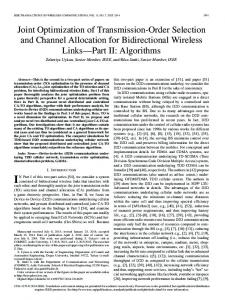
Fig. 2. Dynamic population diversity of ACO algorithms on slowly changing DTSPs with 𝑚 = 0.25 for 10 environmental changes.

where 𝑅 and 𝐸 are defined in Eq. 6 and 𝐷𝐼𝑉𝑖𝑗 defines the diversity of the population in observation 𝑖 of run 𝑗. For the DTSP, 𝐷𝐼𝑉𝑖𝑗 can be calculated as follows:

B. Analysis of the Offline Error Results

𝐷𝐼𝑉𝑖𝑗 =

𝜇 ∑ 𝜇 ( ∑ 𝑐𝐸 ) 1 1 − 𝑝𝑞 , 𝜇(𝜇 − 1) 𝑝=1 𝑛

(8)

𝑞∕=𝑝

where 𝜇 is the size of population, 𝑐𝐸𝑝𝑞 is defined as the number of common edges between the solutions of ants 𝑝 and 𝑞, and 𝑛 is the number of cities.

The experimental results regarding the offline error of ACO algorithms are presented in Table I. The corresponding statistical tests are presented in Table II, where Kruskal–Wallis tests were applied followed by posthoc paired comparisons using Mann–Whitney tests with the Bonferroni correction. In Table II, the results are shown as “−”, “+” or “∼” when the first algorithm is significantly better than the second one, when the second algorithm is significantly better than the first one, or when the two algorithms are not significantly different, respectively. In order to better understand the behaviour of

kroA150, f = 500 8500

4500

6500

8000

4000

6000

3000 2500

1500 0.1

0.5

5500 5000 4500

3500 0.1

0.75

kroA100, f = 5000

0.25

0.5

4500 0.1

0.75

Migration No Migration 0.25

1400

2200

kroA200, f = 5000

3000

800 600

Offline Error

1000

1800 1600 1400 1200

400

Migration No Migration 0.5

0.75

2500 2000 1500

1000 800 0.1

0.75

3500

2000

1200

0.5

m

kroA150, f = 5000 2400

Offline Error

Offline Error

6000

m

1600

0.25

6500

5000

Migration No Migration

m

200 0.1

7000

5500

4000

Migration No Migration 0.25

7500

Offline Error

3500

2000

Migration No Migration 0.25

m

Fig. 3.

kroA200, f = 500

7000

Offline Error

Offline Error

kroA100, f = 500 5000

0.5

0.75

Migration No Migration 1000 0.1

0.25

m

0.5

0.75

m

Offline error of the ℳℳAS(0.8,0.8) algorithm with and without the migration policy.

the algorithms in dynamic environments, their offline error and population diversity against the observations are plotted in Fig. 1 and Fig. 2, respectively, on DTSPs with 𝑓 = 5000 and 𝑚 = 0.25 for 10 environmental changes. From the experimental results, several observations can be made and they are analysed below. First, the single colony ℳℳAS(0.2) outperforms the multi-colony ℳℳAS(0.2,0.2) in most DTSPs; see the comparisons of ℳℳAS(0.2) ⇔ ℳℳAS(0.2,0.2) in Table II. This is because when the evaporation rate is set to a small value the performance of ACO usually is degraded, which can be supported by the performance of ℳℳAS(0.2) against the competing algorithms in Table I. Therefore, the performance is degraded even more in the corresponding multicolony ℳℳAS(0.2,0.2) because more function evaluations are wasted in every environmental change. Second, the multi-colony ℳℳAS(0.8,0.8) outperforms the single colony ℳℳAS(0.8) in most DTSPs; see the comparisons of ℳℳAS(0.8) ⇔ ℳℳAS(0.8,0.8) in Table II. In contrast to the ℳℳAS(0.2) performance, when the evaporation rate is set to a larger value, the performance of ACO is often improved. This can be observed from the offline error results of ℳℳAS(0.2) and ℳℳAS(0.8) in Table I. Usually, faster adaptation (e.g., higher evaporation rate) achieves better performance than slower adaptation (e.g., lower evaporation rate) in most DTSPs. This can be observed from the convergence speed of the two single colony ACO algorithms in Fig. 1. Third, ℳℳAS(0.8,0.8) outperforms ℳℳAS(0.2,0.2) in most DTSPs; see the comparisons of ℳℳAS(0.2,0.2) ⇔ ℳℳAS(0.8,0.8) in Table II. This is inherited by the performance of their corresponding single colony algorithms.

Hence, ℳℳAS(0.8,0.8) and ℳℳAS(0.2,0.2) promote the good and bad performance of ℳℳAS(0.8) and ℳℳAS(0.2), respectively. Although both homogeneous multi-colony ACO algorithms increase the diversity of their corresponding single colony ACO algorithms, which can be observed from Fig. 2, they have different effect on their offline error, which can be observed from Fig. 1. Fourth, the heterogeneous ℳℳAS(0.2,0.8) outperforms ℳℳAS(0.2,0.2) but it is outperformed by ℳℳAS(0.8,0.8) except when 𝑚 = 0.1. This is natural since ℳℳAS(0.2,0.8) inherits the performance of both single colony algorithms (i.e., ℳℳAS(0.2) and ℳℳAS(0.8)). This can be supported by the fact that ℳℳAS(0.2,0.8) outperforms ℳℳAS(0.8,0.8) in all quickly changing environments with 𝑚 = 0.1 because of the good performance inherited by ℳℳAS(0.2); and outperforms ℳℳAS(0.2,0.2) in the remaining DTSPs because of the good performance inherited by ℳℳAS(0.8). C. Analysis of the Effect of Migration The migration task in multi-colony algorithms enables the colonies to communicate. To investigate the effect of migration on multi-colony algorithms, the offline errors of ℳℳAS(0.8,0.8) with and without migration are presented in Fig. 3. From Fig. 3, it can be observed that when migration is enabled, ℳℳAS(0.8,0.8) performs better. Note that similar observations were found for the other multi-colony ACO algorithms, and thus, are not presented in this paper. This is natural because, in case a new best-so-far ant is found, the other colonies are notified via an extra pheromone deposit. Therefore, they are guided towards the promising areas of the search space.

TABLE III.

E XPERIMENTAL RESULTS REGARDING THE OFFLINE BEST ERROR BEFORE A DYNAMIC CHANGE OF ACO ALGORITHMS . B OLD VALUES INDICATE THE BEST RESULTS

Algorithms & DTSPs

kroA100(Optimum=21282)

kroA150(Optimum=26524)

kroA200(Optimum=29368)

𝑓 = 500, 𝑚 ⇒

0.1

0.25

0.5

0.75

0.1

0.25

0.5

0.75

0.1

0.25

0.5

0.75

ℳℳAS(0.2)

751

2357

2992

3158

1971

3912

4706

4855

2826

5180

6022

6214 5318

ℳℳAS(0.8)

974

2052

2451

2510

2356

3593

3965

4061

3537

4832

5272

ℳℳAS(0.2,0.2)

1202

2492

3139

3371

2760

4204

4987

5206

3560

5414

6271

6564

ℳℳAS(0.8,0.8)

1049

2205

2533

2619

2540

3703

4086

4178

3481

4792

5210

5239

ℳℳAS(0.2,0.8)

979

2267

2761

2919

2409

3821

4465

4589

3408

4941

5615

5816

𝑓 = 5000, 𝑚 ⇒

0.1

0.25

0.5

0.75

0.1

0.25

0.5

0.75

0.1

0.25

0.5

0.75

ℳℳAS(0.2)

214

323

470

540

640

903

1103

1103

452

865

1323

1377

ℳℳAS(0.8)

253

360

442

484

666

829

919

958

594

872

1004

996

ℳℳAS(0.2,0.2)

275

368

590

663

779

1209

1422

1447

633

1249

1680

1812

ℳℳAS(0.8,0.8)

166

230

341

350

534

670

775

764

436

581

743

760

ℳℳAS(0.2,0.8)

202

307

427

424

663

895

1037

1052

557

897

1142

1204

When migration is enabled, the colonies promote both cooperation, because information is exchanged via pheromone; and competition, because the best-so-far ant from both colonies is considered. In contrast, when migration is disabled, the colonies are only competing. These observations support our claim that multi-colony algorithms maximize the search area explored; but only when the colonies exchange information. D. Analysis of the Offline Error Before Change In addition to the traditional offline error that measures the adaptability of algorithms for DOPs, the offline best error just before a dynamic change [28] is also used to measure the accuracy of algorithms. The offline best error before change in DOPs is defined as follows: ⎛ ⎞ 𝑀 𝑅 ∑ ∑ 1 1 ¯𝐴𝐶𝐶 = ⎝ 𝐸 (9) 𝐸𝑟𝑟𝑖𝑗 ⎠ , 𝑀 𝑖=1 𝑅 𝑗=1

of multi-colony algorithms are proposed: homogeneous where the colonies have the same behaviour; and heterogeneous where the colonies have different behaviours. The key idea of multi-colony ACO is to maximize the search space explored. The proposed multi-colony ACO algorithms are compared with traditional single colony ACO algorithms on different dynamic test cases of the DTSP. From the experiments, the following conclusions can be drawn. First, the use of parallel colonies improve significantly the performance of ACO for most DTSPs. Second, multi-colony approaches help to enhance the diversity maintenance but they do not always improve the performance. Third, the migration task is important in multi-colony approaches because it enables the communications between the colonies. Fourth, the overall performance (both adaptability and accuracy) of ACO algorithms strongly depends on the difficulty of the DTSP to be tackled.

where 𝑀 is the number of environmental changes, 𝑅 and 𝐸𝑟𝑟𝑖𝑗 are defined as in Eq. (6). Similar to the offline error, the smaller the value, the better the result. For example, a value of 0 means that the algorithm found the optimum on all environmental changes. The experimental results regarding the offline best error before a dynamic change of ACO algorithms are presented in Table III.

Multi-colony ACO algorithms reduce the algorithmic iterations and improve the performance in dynamic environments when the appropriate settings are selected. In evidence, the single colony ℳℳAS(0.8) algorithm performs 10 and 100 iterations when 𝑓 = 500 and 𝑓 = 5000 (i.e., 𝑓 /𝜇), respectively. In contrast, the multi-colony ℳℳAS(0.8,0.8) algorithm performs 5 and 50 iterations on the same environmental cases (i.e., 𝑓 /(𝜇 × 2 colonies)), respectively.

Generally, these results match the offline error results above. The ℳℳAS(0.8,0.8) algorithm performs closer to the optimum followed by ℳℳAS(0.2,0.8) and ℳℳAS(0.2,0.2). However, it can be seen that when the environment changes quickly, the algorithms have larger error than when the environment changes slowly. This is because the available time for the ACO algorithms to re-optimize is shorter. Furthermore, as the magnitude of change increases, the error of the ACO algorithms increases. This shows that severely changing DTSPs are more challenging to tackle than slightly changing DTSPs.

For future work, it would be interesting to investigate more advanced migration policies [21], [29] to exchange information among colonies or even consider more than two colonies. In fact, it has been analysed that smart migration policies lead to significant speedups for parallel evolutionary algorithms in stationary environments [13]. Similarly, the re-optimization time can be improved in dynamic environments when an appropriate communication between colonies is selected. Another future work is to consider other parameters (e.g., 𝛼, 𝛽 or 𝑞0 ) in heterogeneous multi-colony ACO algorithms.

VI.

C ONCLUSION

Multi-colony ACO algorithms have been successfully applied to different optimization problems with stationary environments. This paper investigates the performance of multicolony ACO algorithms in dynamic environments. Two types

ACKNOWLEDGEMENT This work was supported by the Engineering and Physical Sciences Research Council (EPSRC) of UK under Grants EP/K001310/1 and EP/K001523/1.

R EFERENCES [1] D. Angus and T. Hendtlass, “Ant colony optimization applied to dynamically changing problem,” in Developments in Applied Artificial Intelligence, Lecture Notes in Artificial Intelligence, vol. 2358, 2002, pp. 618–627. [2] T. M. Blackwell and J. Branke, “Multi-swarm optimization in dynamic environments,” in EvoWorkshops 2004: Appl. Evol. Comput., Lecture Notes in Computer Science, vol. 3005, 2004, pp. 489–500. [3] E. Bonabeau, M. Dorigo, and G. Theraulaz, Eds., Swarm Intelligence: From Natural to Artificial Systems. New York: Oxford University Press, 1997. [4] J. Branke, Ed., Evolutionary Optimization in Dynamic Environments. Kluwer, 2001. [5] J. Branke, T. Kaußler, C. Schmidth, and H. Schmeck, “A multipopulation approach to dynamic optimization problem,” in Proc. 4th Int. Conf. Adaptive Comput. Des. Manuf., 2000, pp. 299–308. [6] J. Branke and H. Schmeck, “Designing evolutionary algorithms for dynamic optimization problems,” in Advances in Evolutionary Computing, ser. Natural Computing Series, A. Ghosh and S. Tsutsui, Eds. Springer Berlin Heidelberg, 2003, pp. 239–262. [7] M. Dorigo, V. Maniezzo, and A. Colorni, “Ant system: Optimization by a colony of cooperating agents,” IEEE Transactions on System Man and Cybernetics-Part B: Cybernetics, vol. 26, no. 1, pp. 29–41, 1996. [8] C. Eyckelhof and M. Snoek, “Ant systems for a dynamic tsp,” in Proc. 3rd Int. Workshop on Ant Algorithms, Lecture Notes in Computer Science, vol. 2463, 2002, pp. 88–99. [9] L. M. Gambardella, E. D. Taillard, and C. Agazzi, “Macs-vrptw: A multicolony ant colony system for vehicle routing problems with time windows,” in New Ideas in Optimization, 1999, pp. 63–76. [10] M. Guntsch and M. Middendorf, “Pheromone modification strategies for ant algorithms applied to dynamic tsp,” in EvoWorkshops 2001: Applications of Evolutionary Computing, Lecture Notes in Computer Science, vol. 2037, 2001, pp. 213–222. [11] ——, “Applying population based aco to dynamic optimization problems,” in Proc. the 3rd Int. Workshop on Ant Algorithms, Lecture Notes in Computer Science, vol. 2463, 2002, pp. 111–122. [12] Y. Jin and J. Branke, “Evolutionary optimization in uncertain environments - a survey,” IEEE Transactions on Evolutionary Computation, vol. 9, no. 3, pp. 303–317, 2005. [13] A. Mambrini, D. Sudholt, and X. Yao, “Homogeneous and heterogeneous island models for the set cover problem,” in Proc. 12th Int. Conf. on Parallel Problem Solving from Nature - PPSN XII, Lecture Notes in Computer Science, vol. 7491, 2012, pp. 11–20. [14] M. Mavrovouniotis and S. Yang, “A memetic ant colony optimization algorithm for the dynamic travelling salesman problem,” Soft Computing, vol. 15, no. 7, pp. 1405–1425, 2011. [15] ——, “Adapting the pheromone evaporation rate in dynamic routing problems,” in EvoApplications 2013: Applications of Evolutionary Computation, Lecture Notes in Computer Science, vol. 7835, 2013, pp. 606–615.

[16] ——, “Ant colony optimization with immigrants schemes for the dynamic travelling salesman problem with traffic factors,” Applied Soft Computing, vol. 13, no. 10, pp. 4023–4037, 2013. [17] M. Mavrovouniotis, S. Yang, and X. Yao, “A benchmark generator for dynamic permutation-encoded problems,” in Proc. 12th Int. Conf. on Parallel Problem Solving from Nature, Lecture Notes in Computer Science, vol. 7492, 2012, pp. 508–517. [18] L. Melo, F. Pereira, and E. Costa, “Multi-caste ant colony algorithm for the dynamic traveling salesperson problem,” in Proc. 11th Int. Conf. on Adaptive and Natural Computing Algorithms, Lecture Notes in Computer Science, vol. 7824, 2013, pp. 179–188. [19] R. Michel and M. Middendorf, “An island model based ant system with lookahead for the shortest supersequence problem,” in Proc. 5th Int. Conf. on Parallel Problem Solving from Nature - PPSN V, Lecture Notes in Computer Science, vol. 1498, 1998, pp. 692–701. [20] ——, New Ideas in Optimization. Maidenhead, UK, England: McGraw-Hill Ltd., UK, 1999, ch. An ACO Algorithm for the Shortest Common Supersequence Problem, pp. 51–62. [21] M. Middendorf, F. Reischle, and H. Schmeck, “Information exchange in multi colony ant algorithms,” in Parallel and Distributed Processing, Lecture Notes in Computer Science, vol. 1800, 2000, pp. 645–652. [22] ——, “Multi colony ant algorithms,” Journal of Heuristics, vol. 8, no. 3, pp. 305–320, May 2002. [23] T. T. Nguyen, S. Yang, and J. Branke, “Evolutionary dynamic optimization: A survey of the state of the art,” Swarm and Evolutionary Computation, vol. 6, pp. 1–24, 2012. [24] M. Pedemonte, S. Nesmachnow, and H. Cancela, “A survey on parallel ant colony optimization,” Applied Soft Computing, vol. 11, no. 8, pp. 5181 – 5197, 2011. [25] T. St¨utzle and H. Hoos, “The max-min ant system and local search for the traveling salesman problem,” in Proc. 1997 IEEE Int. Conf. on Evol. Comput., 1997, pp. 309–314. [26] ——, “Max-min ant system,” Future Generation Computer Systems, vol. 16, no. 8, pp. 889–914, 2000. [27] E.-G. Talbi, O. Roux, C. Fonlupt, and D. Robillard, “Parallel ant colonies for the quadratic assignment problem,” Future Generation Computer Systems, vol. 17, no. 4, pp. 441–449, 2001. [28] K. Trojanowski and Z. Michalewicz, “Searching for optima in nonstationary environments,” in Proc. 1999 IEEE Congr. on Evol. Comput., vol. 3, 1999, pp. 1843–1850. [29] C. Twomey, T. St¨utzle, M. Dorigo, M. Manfrin, and M. Birattari, “An analysis of communication policies for homogeneous multi-colony aco algorithms,” Inform. Sci., vol. 180, no. 12, pp. 2390–2404, 2010. [30] S. Yang, Y. Jiang, and T. T. Nguyen, “Metaheuristics for dynamic combinatorial optimization problems,” IMA Journal of Management Mathematics, vol. 24, no. 4, pp. 451–480, 2013.