Multi-Layer Network Architecture for Supporting Multiple Applications

Multi-Layer Network Architecture for Supporting Multiple Applications in Wireless Sensor Networks Amjed Majeed1 and Tanveer Zia2∗ 1 School of Mechanical and Electrical Engineering, Sheridan College Toronto, ON, Canada [email protected] 2 School of Computing and Mathematics, Charles Sturt University Australia [email protected] Abstract Traditionally wireless sensor networks’ deployment is meant for a single application, which limits the commercial deployment of a sensor network. In many scenarios, however, it has become desirable to use a sensor network to run multiple applications where the demand for applications that can harness the capabilities of a sensor-rich environment increases. With advancements in sensor technology the size and cost of a sensor node have reduced significantly allowing a large number of resource-constrained sensor nodes be deployed to form a dense network. In order to exploit the dense nature of wireless sensor network by utilizing the available redundant nodes, we propose network architecture made up of three layers, each of which has an equal number of subscribed sets of nodes. An active layer represents the execution of set of nodes running one application. The proposed network architecture to run three applications is designed based on the implementation of scheduling using directed acyclic graph (DAG). The experimental results obtained through Castalia simulation show successful execution of the architecture while maintaining energy efficiency. Keywords: wireless sensor networks; concurrent sensor applications; running multiple applications; multi-layer network architecture

1

Introduction

Advances in wireless networking, micro-fabrication and integration, and embedded microprocessors have enabled a new generation of massive scale sensor networks suitable for a range of commercial and military applications. The technology promises to revolutionize [1] the way we live, work, interact with physical environment. A wireless sensor network (WSN) is composed of a large number of sensor nodes [2] that are densely deployed either inside the field of interest where a phenomenon to be monitored or very close to it. Wireless Sensor Networks when deployed, collectively monitor and disseminate information about a variety of phenomena of interest. Each sensor node is a battery-operated device capable of sensing physical quantities and made up of several parts: a radio transceiver module for wireless communication, memory integrated chip for data and program storage, microcontroller for computation and signal processing, embedded sensing board (temperature, humidity, light, vibration, sound etc.) with electronic interfacing circuit and a battery or an embedded form of energy harvesting. These nodes have emerged as a result of developments in low-power digital and analog circuitry, low-power RF design and sensor technology [3]. Sensor networks are distinct from traditional computing domains; their design assumes being embedded in common environments, instead of dedicated ones. A vast amount (hundreds or even thousands) of Journal of Wireless Mobile Networks, Ubiquitous Computing, and Dependable Applications, 8:3 (September 2017), pp. 36-56 ∗ Corresponding

author: School of Computing and Mathematics, Charles Sturt University, NSW, 2678, Australia, Tel: +61-

2-69332024

36

Multi-Layer Network Architecture for Supporting Multiple Applications in WSNs Majeed, A., Zia, T.

these sensors constitute a wireless sensor network and when these devices are deployed in large numbers, they need the ability to assist each other to communicate data back to a centralized collection point for further data processing and analysis. Advances in integrated circuit design are continually shrinking the size, weight and cost of sensor devices, while simultaneously improving their resolution and accuracy. They are now coming equipped with many adds-on boards, such as sensor board that contains application-specific sensors. The availability of wide variety of sensor boards and sensors such as temperature, air quality, pressure, magnetometers, light, acoustic, accelerometers make WSN popular to serve as a general platform for many application domains solving many practical problems. A WSN has one or more sinks (base-stations) which collect data from all devices. These sinks are the interface through which the WSN interacts with the outside world. The node resource limitations are the primary hindrance in deployment of multiple applications in WSN. We have examined the literature available thus far and proposed preliminary ideas in [4] and [5]. This paper extends on those ideas and supports our proposed algorithms with extensive simulation and experiments as presented in Section 5.

2

Related Work

Initial research work on WSNs was primarily focused on networks running single application or application specific networks and was the start of first generation to be implemented. Challenges posed by WSNs related to deployment, size, and communication protocols as well as scarce resources related to power, memory and processor speed have attracted lots of research work. The new emergence in technology coupled with advances in semiconductor technology have made sensor nodes become more multi-functional devices. Most of WSNs including large scale networks are designed to run single application over the entire network lifetime. Our research has been primarily focused on large dense networks for the ability to execute multiple applications when required. Running single application limits the use of numerous versatile sensor nodes and a major source of system inefficiency even for the purpose of redundancy. Resource wastage in this case is not the only factor, but the design in this case does not fully exploit the enormous capabilities these WSNs possess of self-adapting and self-configuring. The idea of running multiple applications on a single network has gained significant momentum in recent years with lots of research work investigating different effective approaches on design concepts of both hardware and software systems to achieve the goal of running multiple applications on a single network. In [6] the work proposed adds many new challenges to the design and implementation concepts of WSNs since it is not only suggested to run different multiple applications but also with heterogeneous sensor nodes deployed in multiple networks employing multiple base stations and a web server. It is also suggested to have these sensor nodes be part of the new emerging concept Internet of Things (IoT) where sensor data can be accessed through the web. The main challenge in this new trend of multiple applications is the ability to effectively and dynamically coordinate the sharing of available resources for best optimization while at the same time maintaining the goal of meeting application requirements. The authors [6] propose the use of middleware platform solution that can provide high flexibility for adding advanced and sophisticated functions to implement the required algorithms for their approach called service oriented approach. In this approach sensor nodes are considered as service providers and the middleware layer acts as interface between the applications. This would access set of services provided by abstractions of the complex underlying layers through some standard interfaces based on the service-oriented architecture [7]. The work presented in [6] is an algorithm called resource allocation in heterogeneous sensor networks (SACHSEN) which is the core of the resource allocation component of their middleware layer, this algorithm addresses the aforementioned challenges faced by running multiple 37

Multi-Layer Network Architecture for Supporting Multiple Applications in WSNs Majeed, A., Zia, T.

applications onto heterogeneous WSNs. The approach suggested by SACHSEN would seem effective only when the different applications could share the same sensing data when these data have common characteristics in time and space and similar quality of service requirements (QoS), it is not clear how SACHSEN is applied when needs for different data gathered from different sensors. A similar work on scheduling of multiple applications in distributed and heterogeneous networks was also presented in [8], the authors proposed several resource allocation algorithms that carefully constrain the amount of resources that can be allocated to each running application. In [9], the work carried out was for supporting multiple concurrent applications by working out the best trade-off between fidelity-aware resource allocation and the sensor node selection. Fidelity can be defined to represent a concept for an application that can take variety of operational measures such as data quality and communication latency. The trade-off in this case arises when the algorithm starts to reduce the value of fidelity of several tasks in the applications in order to be able to run more simultaneous applications in the WSN system and this result in reducing the quality for that application. The work presented in [10] is an interesting different direction for running multiple applications in WSNs, these deployed networks are aimed to be integrated to the Internet of Things (IoT). The IoT is a networking paradigm evolved on the premise of large scale deployments of two important well-established technologies radio-frequency identification (RFID) and WSNs [11]. With the recent research directions on scalability in WSNs and the emergence of IoT as a new platform that is primarily realized on meeting scalability demands, the integration between the two would make a good optimization of resources. This work would allow WSN significantly benefit from the resource pool that IoT utilizes which comprises of all pervasive technologies and services such as cell phones, CCTV cameras and data collectors. Also, resource sharing and cross-utilization between WSNs and nearby architectures would also give additional benefit to utilize their resources. However, the biggest challenge presented in the paper is how to interweave WSN in the greater paradigm of IoT rather than just to tailor it to work for it. The work proposed aims to move away from WSNs as dedicated systems for sensing tasks to generic platforms of dynamically assigned resources. Nodes in this scenario are viewed as resource providers and the ability to assign measurable attributes to these resources would make it possible to better use them and utilize them to leverage operational capacity across multiple WSN platforms and hence multiple applications could be adopted to run concurrently on different WSNs. The approach idea is divided into three phases: 1) first phase looks into measuring the available resources in the network and their usability 2); the second phase involves representing applications into finite sets of functional requirements and; 3) the last phase looks into optimal mapping between applications and resources. It aims for dynamically accommodating varying resources being introduced or removed as well as utilizing any passing by transient resources in their vicinity. The aforementioned work presented on running multiple concurrent applications with the integration of IoT is a promising trend that will have many research work invested, however there are still many obstacles such as IP address space and allocation to things, availability of sensor nodes on the internet and adapting to large scale and control overhead [12], and challenges that need to be addressed and resolved first in order to translate this into realistic work on ground for implementation. In [13]the authors present a framework to run two applications on a single deployed WSN. The proposed work is for deterministic deployment scenario of wireless sensor nodes in an indoor office building, which assumes the luxury of power replenishment availability to any individual sensor node. The two applications namely Collection and Firecam need to run at different timings, Collection is the default application executed continuously during normal network operation primarily to monitor the building environment parameters such as temperature, humidity, light, and motion PIR detectors. The second application Firecam is executed at emergency event only, specifically when a smoke detector or security sensor goes off in one of the building’s zones. Sensor nodes that happened to be installed in that zone would take a series of picture shots and send them back to the base station. In the second application it can be seen that large amount of data stream need to be transmitted and routed back to the base station. These two scenarios obviously require two different 38

Multi-Layer Network Architecture for Supporting Multiple Applications in WSNs Majeed, A., Zia, T.

configurations with regard to the MAC and network protocols as the first application operates with lowrate reliable many-to-one collection versus the requirement of the second, point-to-point, low-latency, and bulk-data streaming. The authors propose a framework at which design time allows the settings of Network, MAC and Radio protocols for each application as well as the threshold and events that would trigger the WSN reconfiguration. Hence, at run time, the WSN automatically reconfigures itself in response to these events and to the criteria at which they were set at the design stage. In [14], the authors present scoping, a general concept to create node subsets on a network for the purpose of achieving multi-purpose task network. Basically, scoping is achieved by selecting group of nodes through a membership condition such as node properties, for example, nodes that share the same temperature sensing feature can subscribe to one group and so on, this is similar to our work presented since each of dynamic switching set nodes would run different sensing application. In order to delimit the scope of applications to a subset of nodes, the paper mentions that the required separation of applications is made at both node and network levels but it is not clear on how this is implemented. Although this concept is useful to run multiple tasks on a network, however these groups will eventually remain geographically isolated and confined only to their areas in terms of coverage and connectivity and not to the entire network. As well the concept presented may only be applied for deterministic deployment strategy as not clear how this can be implemented when a stochastic type of deployment is required. A similar research study on hosting multiple applications in WSNs is presented in [15]. The paper suggests dynamic allocation of sensor nodes constituting number of groups each of which to host one application. This concept depends on prior knowledge of application characteristics and the state of the network. The information needed in this case will serve as an input is collected from queries and application requests issued by the users of applications. This information is also modeled using a traffic source with stream of application requests following a Poisson arrival process. The requests are then submitted to a proxy stage to process and send request messages to cluster heads in the network. Another work in [16] is carried out on supporting multiple concurrent applications using multi-agent. The authors propose a middleware solution called “SensoMax” that runs on a Java based platforms in a modulated architecture that supports running multiple concurrent applications. Although the proposed SensoMax middleware solution aims to provide high standard features needed for WSN such as Macroprogramming, multi-tasking and multiple concurrent application support, however, it requires the availability of luxury and rich resources in both hardware and software platforms that are rarely available when designing WSN due to the fact that these sensors are characterized by their constrained resources and cost efficiency. The hardware targeted for the sensomax such as Sun Spot and Raspberry Pi [17] are resource-rich hardware platforms for example, Sun Spot devices feature a 400MHz ARM processor, 1MB of data and 8MB of program memory. The paper also discusses dividing the entire area to be monitored into separate regions each of which runs a different application, similar to the concept of scoping discussed in [14] and with that the network connectivity and coverage still of a question if coverage is achieved for the entire network or only confined to the areas on which a specific tasks are being executed. Some new research work has also been focusing on running multiple applications in WSN for multimedia purpose. As we see in [18] work presented to support multiple applications in wireless multimedia sensor networks. The proposed research aims to achieve enabling nodes to transmit audio and video streams along with scalar data. The framework concept is primarily focused on the cross layer architecture for the internal node design concerning network and MAC layers and the associated communication and routing protocols. The design concept works on reserving sufficient amount of memory as a separate space where application specific parameter settings for different layers of the protocol stack are stored and managed by additional middleware layer called Cross Layer Optimization Middleware (CLOM). Those saved parameters and their values are then used by different layers processing data packets for the applications that requested the settings. Despite that fact that Multimedia WSN is a promising future work, however the feasibility of implementing in a harsh sensor environment is still in question as video 39

Multi-Layer Network Architecture for Supporting Multiple Applications in WSNs Majeed, A., Zia, T.

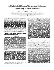
Figure 1: A graph representing a distributed system data streaming in particular requires a robust and reliable wireless channel with sufficient bandwidth and data rate as well as back-up power sources for the high energy consumption in this case. A thorough analysis of the related work is provided in Table 1.

3

Network Model

Models for wireless sensor networks are needed to develop algorithms mathematical correctness representations. Since the topology of a wireless sensor network can be regarded as a graph, models from graph theory can be used, Directed Acyclic Graph (DAG) is one which is implemented in our proposed work. DAG, sometimes referred to task graph is a commonly implemented model to represent task scheduling. The scheduling of a task implies that some precedence constraints need to be satisfied prior to running/execution of a task. A distributed system such as wireless sensor network can be modeled as a graph G(V, E) where V is the set of vertices and E is the set of edges of G. The computing nodes of the WSN are represented by the vertices of the graph, and an edge exits between the nodes if there is a communication link between them. Figure 1 shows a general graph of a distributing system consisting of 7 nodes, numbered 1 to 7. It can be seen that the graph is connected, providing a communication path between any pairs of nodes. If the vertex set V of a graph G is finite then it is called a finite graph, the assumption used throughout the work. An edge is identified by two vertices, and the edge is said to be incident to the vertices, as an example, edge e = {v1 , v2 }, sometimes written as e = v1 v2 or e{ v1v2}, is incident to the vertices v1 and v2 . The proposed network model follows directed graph on a two-dimensional plane. A directed graph (digraph) G(V, E) consists of a nonempty set of vertices V and a set of directed edges E where each e ∈ E is associated with an ordered set of vertices [19] An edge e is associated with the ordered pair (u, v) is described as starting from u and ending at v. Figure 2, shows a digraph with V = {1, 2, 3, 4} and E = {{1, 2}, {2, 4}, {3, 2}, {3, 4}, {4, 3}, {4, 1}} In a diagraph, we call u the tail of e, v the head of e, and u, v the end of e, if there is an edge with tail u and head v, then we let (u, v) denote such an edge and the edge becomes directed from u to v. If an edge e = (u, v) in a direct graph V is such that u = v then this is called a loop. Edges e, f are parallel if they have the same tails and heads. An important relationship in a diagraph is defined where a vertex u is called the predecessor of vertex v and the corresponding v is called the successor of u, if only if edge euv ∈ E, u, v ∈ V . 40

Multi-Layer Network Architecture for Supporting Multiple Applications in WSNs Majeed, A., Zia, T.

Figure 2: A directed graph

The vertex - edge concept of a direct graph in a WSN results in a node mimics a vertex where computation and sensing activities take place; the edge mimics communication link in this case. The time spent by a node (vertex) on a task computation/sensing and communication (edge) is a measure for cost which is incorporated in a graph model by assigning weights to its elements. The nonnegative weight s(v) represents sensing/computation cost and is associated with vertex v ∈ V and the nonnegative weight c(v) represents communication cost and is associated with edge e ∈ E. The above-mentioned definitions are the foundation for task scheduling towards application execution on a single wireless network. The mechanism for running applications sequentially is manifested by direct acyclic graph DAG as follows: directed acyclic graphs are directed graphs that have no cycles. If an edge ei, j = (vi , v j ) exits from node vi to node v j , then vi is called the parent of v j and v j is called the child of vi . If vi is the parent of v j and v j is the parent of vk then we say that vi is the ancestor of vk and vk is the descendant of vi . Following up the above-mentioned definitions, the properties of DAG can be summarized as: 1. The structure consists of nodes and edges, where edges are unidirectional 2. The direct relationship between any two nodes is represented by a maximum of one edge. 3. Indirect relationships, or paths, between any two nodes may exist through edges with other nodes. 4. Each node may have one or more child nodes and each node may have one or more parent nodes. 5. There may exist ancestor nodes for any given node, which consist of all the successive parents of a node. 6. There may exist descendant nodes for any given node, which consist of all the successive children of a node. 7. There exists an inverse structure to any given acyclic diagraph structure, which is the same structure but with all the edge directions reversed. We implemented DAG scheduling concept to our proposed network model as follows: 1- Phase 1, high level scheduling, coordination between Base Station (BS) and three Network Layers, 41

Multi-Layer Network Architecture for Supporting Multiple Applications in WSNs Majeed, A., Zia, T.

Concurrency & Programming at Network Level

Concurrency & Programming at Group

Concurrency & Programming at Node Level

Table 1: Comparative analysis of the related work TinyOS/nesC Allows concurrency at Node level and letting processor sleep as much as possible due to event-driven and hence, energy efficiency. Complexity since no blocking operation

TinyThread Y-Thread Melete Impala SensorWar Efficient per- Shared stack for A tiny virtual Supports concurrency at thread stack computation and machine archi- both node and network allocation as separate stack tecture. Stack level. It is also based on it uses stack for control. It is oriented on top Mate virtual machine conestimator. It is often too expen- of TinyOS. Had cept & Both are middleware often too expen- sive in terms of limited flexibility based. Impala allows softsive in terms of memory to stat- and minimal ware to be updated dynammemory to stat- ically allocating support for con- ically. Sensorware supports ically allocating per-thread stack. currency. These Tcl-based script language per-thread stack. With the blocking issues were then for re-programmability With the blocking execution con- addressed by ap- However, they require the execution con- texts, simplifies plication specific luxury of more memory texts, simplifies programs virtual machine. since they were designed for programs. iPAQ pocket pc devices. Neighborhood-based Group Logical Group These are defined by physical closeness. Abstract These are based on sharing some logical properties Regions and Hood provide programming primitives such as node type and sensor reading. These logical based on neighborhood. Neighborhood based groups groups are more dynamic as the group membership is are mostly static. often determined by dynamic properties such as sensor input. Group level abstraction feature the good collaboration among sensors as they support aggregation at group level through data sharing as well as being efficient within the group, however, we think when it comes to multi-application running, it would be very sophisticated to control and managing multi-application due to the nature of distributed groups. Database Other Network level reprogramming and concurrency Cougar and Run-Time Dynamic Linking is another work [4] for reprogrammability in wireless sensor netTinyDB are works where system functionality update is achieved. The intended design is to update native two examples code in heterogeneous network. This work implements an in-situ run time dynamic linker and of network- loader that use the standard Executable Linking File object (ELF Object) file format. Although ing level. run-time dynamic linking a great approach for WSN, its main drawback lies in the need of speWhile their cial compressor utility for creating a compact ELF(CELF) as the ELF object file needs to be in-network compressed to accommodate the 8-bit & 16-bit processors. Part of our proposed work is based query pro- on Agilla mobile agent middleware for sensor networks that establish in-network programming. cessing and Their architecture is based on tuple spaces and neighbor lists for agent coordination. Our proposed collabomodel follows a similar approach to Agilla but with some modifications. The agent manager in ration are Agilla architecture can handle a maximum of three agents due to limitation of processor speed declaratively and memory availability. Also Agiila uses two types of operations WEAK and STRONG operdescribed ation. Since the STRONG operation suffers higher overhead we have only adopted the WEAK by query, Operation and also limited our architecture design to two agents to free memory space and to be these are in line with processor speed. Since Agillas’ mobile agents are continuously on the move migratonly suitable ing and cloning as required for example for updates, configuration and new application code, they for describ- are heavily dependent on wireless links in the network which is somehow unreliable and hence ing query affects its efficiency and reliability. In our proposed design we have implemented lightweight operations mobile agents that would only act as an ON-OFF control in most cases. This uses less energy to a sensor transmission when compared to Agillas’ mobile agents. network.

Network Layer1, Network Layer2 and Network Layer3. 2- Phase 2, low level scheduling, coordination between each network layer and its subscribed sensors, S1 , S2 , ...., Sn . 42

Multi-Layer Network Architecture for Supporting Multiple Applications in WSNs Majeed, A., Zia, T.

Phase1 – High Level Scheduling Phase 01 Three network layers assigned to run three applications in a predetermined sequence. The subscribed sets of nodes of each layer become active running one application when the layer schedule is due as set by the BS. NL1 begins the execution of first application during which the other two layers are sustained in energy saving modes. Subject to the task completion of NL1, the second layer NL2 begins executing the second assigned task/application as scheduled. Finally, NL3 goes active when the previous two network layers NL1 and NL2 have completed their assigned task/application. The coordination between each NL and BS is established by the planner software running at the BS. The following parameters describe the concept of layering and partitions: Definition 3.1: Network Layer (NLx) is a collection of all sets that are scheduled to run one application such that: NL1 = {S1 , 1, S1 , 2, S1 , 3. . . . . . ..S1,n } NL2 = {S2 , 1, S2 , 2, S2 , 3. . . . . . ..S2,n } NL3 = {S3 , 1, S3 , 2, S3 , 3. . . . . . ..S3,n } Definition 3.2: A cover of a graph G(V, E) for running one application is a collection of all sets of nodes that belong to the network layer of that application, such that: n [

Si = V = NL

i=1

Definition 3.3: The size Z(S) of a set S is the number of nodes in S. The hexagon shape represents the sensing field of interest in Figure 3 where Network Layer (NL1) is active and running first application while other two layers are in sleeping energy saving mode. The collection sets of active nodes in a layer is represented by a 3D block to highlight application running as scheduled by the BS, here we have NL1 being active (S1 , 1, S1 , 2, S1 , 3. . . . . . ..S1,n ). Similarly, when NL2 is active the other two network layers NL1 and NL3 will be in saving mode and so on.

Phase 2 – Low Level Scheduling Since each layer is comprised of a number of sets, the scheduling propagates from each layer to its subscribed sets of nodes. A sensor in any set will only start the sensing function once its predefined precedence constraints are met. The base station through NL begins communicating with for example node1 to start its sensing function and that its schedule is now due. Meanwhile all other sensors in the set remain inactive until the predefined schedule criteria of each is met. Next node will begin functioning once it receives a copy of the BS start flag from, it makes a copy and begins its sensing duty. Similarly scheduling of node3 begins once node1 and node 2 started and received start flag and so on until all nodes in the set have received the initializing starting ‘start flag’ sent by BS. This is shown in Figure 4. Basically, it implements a topological ordering that satisfies the precedence constraints. In Figure 4, Node1 closest to the BS is considered cluster head (CH) of the set in NL1 (since it requires minimum energy consumption for communication with the BS). At the start the BS communicates with CH and sends a copy of the starting protocol flag to begin sensing duty. The CH would subsequently sends a replicate copy to all sensors in the set for initialization and implementing the topological ordering

43

Multi-Layer Network Architecture for Supporting Multiple Applications in WSNs Majeed, A., Zia, T.

Figure 3: Sensing field represented by three network layers comprising of sensor node sets

Figure 4: A set of network layer showing the task scheduling of nodes with the base station coordination.

44

Multi-Layer Network Architecture for Supporting Multiple Applications in WSNs Majeed, A., Zia, T.

Figure 5: Hierarchy of System Network Algorithm

4

Network System Algorithm

The general hierarchy of the proposed system algorithm is shown in Figure 5. It comprises of the following: 1- Software planner (coordinator) built at the base station 2- Three virtual network layers (Network Layer 1, Network Layer 2, and Network Layer 3) managed by software planner 3- Each network layers (1,2, & 3) is made up of equal number of sets ( Set1 , Set2 , . . . , Setn ) 4- Each set contains equal number of subscribed sensor nodes

4.1

Network System Pseudocode

Sensors nodes are deployed to the sensing field of interest with base station loaded with software planner. Base station begins initialization phase of identifying sensors that make up sets and the sets that make up each network layer. Cluster heads are identified for each set in a network layer (normally closest to BS is selected, Node1) We make the following assumptions about the network.

45

Multi-Layer Network Architecture for Supporting Multiple Applications in WSNs Majeed, A., Zia, T.

Algorithm 1 for NLx = 1 to 3 do for Si = 1 to n do Cluster Head (Node1) is identified and communication is established with BS Copy of Sensing Protocol, schedule due, and start flag is propagated to all nodes in set Si . Now that all sensors, sets and layers have been identified, also their schedule and application tasks have been propagated, the next step is to implement the sequential running of each application by BS. while NL1 schedule active do Application/Task 1 is running NL2 and NL3 sensor node sets are in sleeping energy saving mode while NL2 schedule active do Application/Task 2 is running NL1 and NL3 sensor node sets are in sleeping energy saving mode while NL3 schedule active do Application/Task 3 is running NL1 and NL2 sensor node sets are in sleeping energy saving mode

• Transmission range (rc ) for each sensor node is fixed. • Sensor nodes have identical energy and are densely deployed in monitored region • Sensor nodes are randomly and uniformly deployed in a planar field. • Base station and sensor nodes are static and aware of their locations via a localization technique [20]. • One application to run at a time in a predefined logical sequence coordinated between base station and cluster heads in the sets of network layers. We also introduce number of parameters that we used but not restricted to in the proposed algorithm as follows: • Total sensing area or field of interest is (A) • Density of nodes are of a uniform distribution (pn ) • Number of applications designed to run on single network is given by (m), 3 in our case. • Node communication range (rc ) in Omni-direction • Node sensing range is a unit disk (rs ) such that :rc ≥ 2rs

4.2

Network Layer and Sets’ Construction

First, the sensing field is divided into equal areas called Set1 , Set2 , . . . ., Setn .The ‘n’ sets are then rearranged into three overlapping groups named network layers 1, 2, and 3. Each layer with associated sets is responsible to run one application on a predefined logical sequence. When network layer1 is active running application, sets of the two other layers have their nodes in sleeping mode (energy saving mode). During the execution of an application, active nodes are also covering adjacent areas whose sensor nodes 46

Multi-Layer Network Architecture for Supporting Multiple Applications in WSNs Majeed, A., Zia, T.

are in sleeping mode, our approach is we establish the necessary and sufficient conditions for coverage to imply connectivity [21]. 1- Let A be a convex area representing the sensing field of interest (FOI) 2Let K be the number of subareas partition sets of A where each partition is called a set such that: S1 , S2 , S3 , . . . ..SK f or a given K ≥ 1

(1)

3- Assume number of sensor nodes ‘n’ is uniformly distributed in A. Sensor nodes in each set are involved in the following: I. Sensors in each set can form a cluster itself II. Sensors in each set either active running application or in energy saving sleep mode queuing for the next in-line application. III. Active running sensors maintain coverage of neighboring partitions whose nodes are in a sleeping mode. 4- Since sensor nodes in each set (S) form a cluster, 1 ≤ i ≤ k let p1 , p2 , ..., pk be the probabilities of sensor nodes located at S1 , S2 , S3 , . . . ..SK respectively [22]. P(n1 , n2 , . . . .nk ) =

n! pn1 pn2 . . . . . . .pnk k (n1 !, n2 !. . . .nk !) 1 2

(2)

n n := ∑Ki=1 ni , : is the number o f sensors in the network If N1 , N2 , . . . .NK have a multinomial distribution with parameters n, and p1 , p2 , . . . .pK , then the expected number of sensor nodes within each cluster E(Ni ) = n. To obtain an equal number of sensor nodes in each cluster, we have p1 = p2 = ...pk which can only be achieved if S1 = S2 = ...Sk in terms of areas, assuming that the density function of sensor nodes in the sensing area is uniformly distributed. 5- Let each sensor node has a communication range (rc ) in Omni-direction 6- Let each sensor node has a sensing range a unit disk (rs ) such that: rc ≥ 2rs

(3)

We introduce a new sensing range parameter. This parameter is calculated such that sensing scope of each sensor when active covers adjacent neighboring areas. This new calculated sensing range depends on number of applications designed to run on a network (three in our case). The formula for the new sensing range of a node is given below: r0s =

rs m

(4)

where 1 ≤ m ≤ 3 Number of applications to run) Where: r0s is the new sensing range used by each node, m is the number of applications running on the network 7 – Let the perimeter of the sensing field be given by Ps in meters Therefore the number of partitions is K and is given by: ps (5) K= r0s The value of K returns the number of partitions and hence sets need to be formed in order to maintain coverage when one network layer is active. 8 - The area of each set can now be found as follows: SA =

A K

(6)

9 - Number of sensor nodes needed per set can be approximately calculated as follows: pSet = 47

SA πr0s

(7)

Multi-Layer Network Architecture for Supporting Multiple Applications in WSNs Majeed, A., Zia, T.

10 – From equation (4.7) we can calculate approximately the total number of nodes needed to be deployed for our convex sensing field nr = pSet × K (8) 11- Let the sensor nodes at the boundary of the sensing field be B. The algorithm divides the sensing field into equal subareas (sets) by radial lines from the center of the field; this part of algorithm requires the location of all sensor nodes at the boundary of the sensing field area as an input given by B. Those boundary nodes are found using Graham’s scanning algorithm [23] for the given convex polygon (P). In this polygon each sensor node is either on the boundary or inside the polygon of the sensing field. The polygon area A (sensing field) is calculated using boundary sensor nodes locations: (Xi ,Yi ), 1 ≤≤ Pn

(9)

Where: Pn is the number of boundary sensor nodes and (Xi ,Yi ) is the location of a boundary sensor node. Assume the location of sensor node (XPn+1 ,YPn+1 ) is (X1 ,Y1 ). The area AP (area A of convex polygon P) and the centroid location of the polygon can be found as follows [24]: 1 Pn ∑ (XiYi+1 − Xi+1Yi ) 2 i=1

(10)

X0 :=

1 Pn ∑ (Xi + Xi+1 )(XiYi+1 − Xi+1Yi ) 6A p i=1

(11)

X0 :=

1 Pn ∑ (Yi +Yi+1 )(XiYi+1 − Xi+1Yi ) 6A p i=1

(12)

A p :=

The partition/Set procedure selects an arbitrary sensor node on the boundary B as the starting point P1. Then selects sensor node P2 on the boundary in ant-clockwise order. The area bounded by P1, P2, and the centroid P0 is calculated using equation (1). If the area is greater than the AC L (SA area of each set given in equation ??). This means the required area must be bounded by P0, P1 and intermediate point (a virtual sensor node) Pv that lies on the P1P2 line. Making use of set area and the locations of P0, P1 and P2, the location of Pv (X and Y coordinates) is calculated as follows: YV :=

Y1 −Y0 Y1 −Y0 X0 +Y0 − X0 X1 − X0 X1 − X0

(13)

1 (X0YV − 2SA ) Y0

(14)

XV :=

If the calculated partition/Set is less than the previously calculated set area (equation 6) a new sensor node on the boundary of sensing field next to P2 needs to be added and the area is recalculated. Ultimately, the sensor nodes of the boundary of the k partitions/Set are stored in BCL.

4.3

Network Layer Nodes’ allocation

The next stage is to identify and locate which node reside in which partition. An algorithm [5] is developed to address this: a) Each partition (Set) is a sector that constitutes a certain angle θSi . This angle is bounded by three points, the centroid and the two vertex points that make up the sector, e.g. 6 P2 P0 P1 as shown in Figure 6. 48

Multi-Layer Network Architecture for Supporting Multiple Applications in WSNs Majeed, A., Zia, T.

Figure 6: The angle θ shown for a Set partition

b) The algorithm first calculates the angle of each particular Set sector and identifies its three points for example in a counterclockwise P2P0P1 as shown in Figure 6. It would then start to randomly pick a node within the neighborhood area adjacent to the sector. The selected node becomes the new vertex point “PZ ” which would repeat with every new node chosen in this area. Each time a new node selected, an internal counter is incremented that keeps track of roughly the total number of nodes in each Set and not to exceed the predetermined population of a Set. The new PZ vertex now makes a new angle with the other two fixed node points for this sector measuring in counterclockwise direction 6 P2 P0 P1 as shown in Figure 7. c) If the new calculated angle from the new node is measured less or equal to the original sector angle then this sensor node is either inside or on the boundary of the Set sector and hence belongs to this sector. It is identified and given an ID that reflect its membership to this Set. d) If however the new measured angle is bigger than θSi then it will be ignored as it resides outside that specific Set and belongs to the adjacent sectors. e) Then the next node is chosen and the same algorithm is applied. The node selection and angle comparison process is repeated continuously until the number of identified nodes for a particular Set reaches the estimated pre-calculated number (compared with internal counter) of nodes that need to be residing in each Set. f) The next Set sector runs the same set of steps of the algorithm above until all the sectors in the 49

Multi-Layer Network Architecture for Supporting Multiple Applications in WSNs Majeed, A., Zia, T.

Figure 7: Node allocation procedure to each Set sensing area identify their actual nodes in their jurisdictions.

4.4

Network Layer Cluster Heads Formation

Now we need to determine cluster heads (CHs) candidates in each set of the network layer. Our algorithm is based on a homogenous sensor network, a network in which all the nodes have identical hardware capabilities [25]. The cluster heads are responsible for collecting data from other nodes in the cluster, performing data aggregation, [25–27] to the remotely located base station. In order to ensure load balancing and uniform energy drainage pattern across the entire network, it is proposed to establish a rotating role of cluster heads on the nodes. Each cluster head CH would store all information related to node IDs residing in a set. We haver the transmission range for each sensor node; there is a strong relationship between the Euclidean distance d from the sender (a sensor node) to the receiver (its cluster head) and the number of hops within distance d. Each route from a sensor node to its cluster head must meet: Number o hops in a shortest path ≥ 50

d r

(15)

Multi-Layer Network Architecture for Supporting Multiple Applications in WSNs Majeed, A., Zia, T.

Table 2: Running - Three Applications Total Network Time Simulation = 60Sec (39 Nodes + Sink) NL Group 1 = 0-20 Sec — NL Group 2 = 21-40 Sec — NL Group 3 = 41-60 Sec Node NL 1 NL 2 NL 3 Node NL 1 NL 2 NL 3 Node ID (#Pack- (#Pack- (#Pack- ID (#Pack- (#Pack- (#Pack- ID ets) ets) ets) ets) ets) ets) 1 0 20 0 14 0 0 20 27 2 0 0 20 15 20 0 0 28 3 20 0 0 16 0 20 0 29 4 0 20 0 17 0 0 20 30 5 0 0 20 18 20 0 0 31 6 20 0 0 19 0 20 0 32 7 0 20 0 20 0 0 20 33 8 0 0 20 21 0 20 0 34 9 20 0 0 22 20 0 0 35 10 0 20 0 23 0 0 20 36 11 0 0 20 24 0 20 0 37 12 20 0 0 25 20 0 0 38 13 0 20 0 26 0 0 20 39

NL 1 (#Packets) 20 0 0 20 0 0 20 0 0 20 0 0 20

NL 2 (#Packets) 0 20 0 0 20 0 0 20 0 0 20 0 0

Table 3: Application: Packets received per group 1 2 3 260 258 247 Most routing protocols use hop counting as one of the route selection criteria. These protocols aim to minimize the number of transmissions required to send a packet along the selected path. In addition, if the network is a dense network as in our case, then the minimum number of hops in the shortest path approaches d/r. To minimize the number of hops between a CH and its sensor nodes, the maximum distance between them need to be minimized. Accordingly, it is assumed that the center of a cluster area is the best location of the cluster head, which balances energy consumption among the sensor nodes in the partition/cluster, using equations (1), (11) and (12), and the location of each CH in each partition is calculated.

4.5

Application running on a Network Layer

The software planner (coordinator) at the base station keeps an ordered list of sequence of 3-tuple list for executing three applications. Soon after network initialization, network hierarchy of layers and sets are established, the base station initiate set of commands to cluster heads to all Sets pertaining Network Layer 1. Nodes in network layer 1 begins running application 1, Meanwhile, nodes pertaining to all other sets of the two other network layers transit to energy saving mode (sleep mode) queuing for next in line application [28]. Active nodes of once complete task/application, they move to sleep mode allowing next application in queue to run on sets pertaining to Network Layer 2 while Sets of Network Layer 3 remain in sleep mode. Finally, application 3 starts once application 2 is complete.

Table 4: Application: Packets received per node in any 20 seconds time period Per node 19.615 51

NL 3 (#Packets) 0 0 20 0 0 20 0 0 20 0 0 20 0

Multi-Layer Network Architecture for Supporting Multiple Applications in WSNs Majeed, A., Zia, T.

Table 5: Application: Packets received per node in any 20 seconds time period Per node 59.242

Figure 8: Active Sensor Nodes of Network Layer One Running Application One

5

Simulation and Experimental Results

Our experimental results are based on simulation of 40 sensor nodes (39 + sink) using Castalia Simulator. Castalia is a popular simulator ideal for Wireless Sensor Networks (WSN), Body Area Networks (BAN) and networks of low-power embedded devices. It is based on the OMNeT++ platform which is used by researchers and developers to test distributed algorithms and protocols in realistic wireless channel and radio models. It also gives a realistic node behavior when accessing the radio model [29]. In this model, the variability of the wireless channel sigma, communication links, and packet collisions have been removed and set to ideal for the purpose of validating the proposed algorithms associated with of different network layers. The experimental results as given in Table 2 are for three applications executed on 39 nodes communicating with base station over 60 seconds network lifetime. On completion of sensor allocation process, each network layer began running one application in a predefined sequence set by the base station, packets exchange between active nodes the base station are recorded for each layer. During the first time span of 20 seconds, the first thirteen sensor nodes of network layer 1 (NL1) communicated on average of 20 packets per node to the base station, while sensor nodes of the two network layers 2 and 3 are in sleeping mode. The second Layer becomes active running application 2 during the time span of the network life time from 21-40 seconds while nodes of Network Layers1 and 3 transits to sleep mode. The third set of nodes under layer 3 scheduled to run application 3 become active during the last and third time span from 41-60 seconds. The total packets of all sensor nodes in each layer communicated to base station is shown in Table 3 in which 260 , 258 and 247 packets are delivered to base station by network layer 1, 2 and 3 respectively. This shows that the average number of data packets sent by each node in any active group is approximately 20 packets during a period of 20 seconds verifying the packet rate of 1packet/sec. Table 4 shows the average number of packets (19.615 packets) sent to the base station by each node in 52

Multi-Layer Network Architecture for Supporting Multiple Applications in WSNs Majeed, A., Zia, T.

Figure 9: Active Sensor Nodes of Network Layer Two Running Application Two

Table 6: Application: Remaining energy Per node 98.246

any 20 seconds time period while Table 5 shows the average number of packets (59.242 packets) sent by an individual node over the complete network life time of 60 seconds. As previously discussed each of the three applications is executed on a group of 13 sensor nodes that are subscribed to one Network Layer. When each group is active and running one application, nodes of the two other groups are transmitted to energy saving mode, Figure 8, Figure 9, and Figure 10 show list of node IDs for each Network Layer respectively when active running one application during the network lifetime. Total of 13 Nodes in Figure 8 above have been identified by the BS to comprise NL1 running first application. These NL1 nodes have IDs start N3, N6, N9, N12, N15, N18, N21, N24, N27, N30, N33, N36 and N39. Similary, 13 nodes for the other two layers NL2 and NL3 have their IDs shown in Figure 9 and Figure 10 respectively. We have also measured energy related metrics in Joules pertaining to nodes consumed and remained energy over the simulation time of 60 sec, given that the initial energy of each node was set to 100J. Tables 6 and 7 show the remained and consumed amount of energy by each node at the end of 60 sec life times respectively. Table 8 shows the total sum of remained energy of 13 nodes in each network layer during any 20 sec time period.

Table 7: Resource Manager: Consumed Energy Per node 1.754 53

Multi-Layer Network Architecture for Supporting Multiple Applications in WSNs Majeed, A., Zia, T.

Figure 10: Active Sensor Nodes of Network Layer Three Running Application Three Table 8: Application: Application: Remaining energy per group 1 2 3 1277.8 1277.79 1279.29

6

Conclusion

This paper has addressed some primary issues related to the limitations of running a single application on a dense WSN when deployed in the field of interest. One of the main issues in a dense network running a single application is the waste of resources when it comes to consider that extra nodes are deployed to serve redundancy purpose, and the issue of total cost pertaining to a return of interest that is directly related to the ‘usefulness’ of the network deployed. Addressing these issues, coupled with the high market demand to have a single network able to perform multiple task functions, we have proposed a three layer network architecture. Each layer (NL1, NL2 and NL3) to have a number of subscribed nodes run one application during a predefined set sequence and time schedule implemented by the software planner in the base station. When one layer is executing one application, the two remaining layers transit to energy saving mode (sleeping mode) to conserve energy while waiting for their application schedule execution sequence to start. We have implemented the proposed algorithm on Castalia simulator and the results obtained are very promising. The required number of nodes to be deployed is an important element to be considered when deploying a WSN, and plays a key role in achieving our proposed goal of running multiple applications on a network.

References [1] F. Zaho and L. J. Guibas, Wireless Sensor Networks, An Information Processing Approach. Elsevier, 2004. [2] S. Slijepcevic and M. Potkonjak, “Power efficient organization of wireless sensor networks,” in Proc. of the 2001 IEEE International Conference on Communications (ICC’01), Helsinki, Finland. IEEE, June 2001, pp. 472–476.

54

Multi-Layer Network Architecture for Supporting Multiple Applications in WSNs Majeed, A., Zia, T.

[3] J. Cho, G. Kim, T. Kwon, and Y. Choi, “A distributed node scheduling protocol considering sensing coverage in wireless sensor networks,” in Proc. of the 66th IEEE Vehicular Technology Conference (VTC’07), Baltimore, Maryland, USA. IEEE, September 2007, pp. 352–356. [4] A. Majeed and T. A. Zia, “Multi-set architecture for multi-applications running in wireless sensor networks,” in Proc. of the 24th IEEE International Conference on Advanced Information Networking and Applications (AINA’10), Perth, Western Australia, Australia. IEEE, April 2010, pp. 20–23. [5] A. Majeed and T. A. Zia, “DSS: Dynamic switching sets for prolonging network lifetime in sensor nodes,” in Proc. of the 37th IEEE International Conference on Local Computer NEtworks Workshops (LCN Workshops’12), Clearwater, Florida, USA. IEEE, October 2012, pp. 22–25. [6] W. Li, F. Delicato, P. Pires, Y. Lee, A. Zomaya, and C. Miceli, “Efficient allocation of resources in multiple heterogeneous wireless sensor networks,” Journal of Parallel Distributed Computing, vol. 74, no. 1, pp. 1775–1788, January 2014. [7] N. Mohamed and J. Al-Jaroodi, “A survey on service-oriented middleware for wireless sensor networks,” Service Oriented Computing and Applications, vol. 5, no. 2, pp. 71–85, June 2011. [8] T. NTakpe and F. Suter, “Concurrent scheduling of parallel task graphs on multi-clusters using constrained resource allocations,” in Proc. of the 2009 IEEE International Symposium on Parallel and Distributed Processing (IPDPS’09), Rome, Italy. IEEE, May 2009, pp. 1–8. [9] N. Roy, V. Rajamani, and C. Julien, “Supporting multi-fidelity-aware concurrent applications in dynamic sensor networks,” in Proc. of the 8th IEEE International Conference on Pervasive Computing and Communication Workshops (PERCOM Work-Shops’10), Mannheim, Germany. IEEE, March 2010, pp. 43–49. [10] S. Oteafy and H. Hassanein, “Towards a global iot: Resource re-utilization in wsns,” in Proc. of the 2012 International Conference on Computing, Networking and Communications (ICNC’12), Maui, Hawaii, USA. Networking and Communications, January 2012, pp. 617–622. [11] A. Castellani, N. Bui, P. Casari, M. Rossi, Z. Shelby, and M. Zorzi, “Architecture and protocols for the internet of things: A case study,” in Proc. of the 8th IEEE International Conference on Pervasive Computing and Communications Workshops (PERCOM’10), Mannheim, Germany. IEEE, May 2010, pp. 678–683. [12] D. Guinard, V. Trifa, F. Mattern, and E. Wilde, “From the internet of things to the web of things: Resource oriented architecture and best practices,” in Architecting the Internet of Things, D. Uckelmann, M. Harrison, and F. Michahelles, Eds. Springer Berlin Heidelberg, 2011, pp. 97–129. [13] M. Szczodrak, O. Gnawali, and L. Carloni, “Dynamic reconfiguration of wireless sensor networks to support heterogeneous applications,” in Proc. of the 2013 IEEE International Conference on Distributed Computing in Sensor Systems (DCOSS’13), Cambridge, Massachusetts, USA. IEEE, May 2013, pp. 52–61. [14] J. Steffan, L. Fiege, M. Cilia, and A. Buchmann, “Towards multi-purpose wireless sensor networks,” in Proc. of the 2005 Systems Communications, Montreal, Quebec ,Canada. IEEE, August 2005, pp. 336–341. [15] N. K. Kapoor, B. Nandy, and S. Majumdar, “Dynamic allocation of sensor nodes in wireless sensor networks hosting multiple applications,” in Proc. of the 2013 International Symposium on Performance Evaluation of Computer and Telecommunication Systems (SPECTS’13), Toronto, Ontario, Canada. IEEE, July 2013, pp. 51–57. [16] M. Haghighi and D. Cliff, “Multi-agent support for multiple concurrent applications and dynamic datagathering in wireless sensor networks.” in Proc. of the 7th International Conference on Innovative Mobile Internet Services in Ubiquitous Computing (IMS’13), Taichung, Taiwan. IEEE, July 2013, pp. 320–325. [17] E. Upton and G. Halfacree, Raspberry Pi: USER GUIDE IS. John and Sons: Wiley, 2012. [18] M. Farooq, T. Kunz, and M. St-Hilaire, “Cross layer architecture for supporting multiple applications in wireless multimedia sensor networks,” in Proc. of the 7th International Wireless Communications and Mobile Computing Conference (IWCMC’11), Istanbul, Turkey. IEEE, July 2011, pp. 388–393. [19] K. Erciyes, Distributed Graph Algorithms for Computer Network. Computer Communications and Networks, 2013. [20] N. Bulusu, J. Heidemann, and D. Estrin, “Gps-less low cost outdoor localization for very small devices,” IEEE Personal Communication Magazine, vol. 7, no. 5, pp. 28–34, October 2000. [21] H. Zhang and J. Hou, “Maintaining coverage and connectivity in large sensor networks,” Ad Hoc & Sensor Wireless Networks, vol. 1, no. 1/2, pp. 89–124, 2005.

55

Multi-Layer Network Architecture for Supporting Multiple Applications in WSNs Majeed, A., Zia, T.

[22] O. Jerew and W. Liang, “Prolonging network lifetime through the use of mobile base station in wireless sensor networks,” in Proc. of the 7th International Conference on Advances in Mobile Computing and Multimedia (MoMM’09), Kuala Lumpur, Malaysia. IEEE, December 2009, pp. 558–659. [23] R. Graham, “An efficient algorithm for determining the convex hull of a finite point set. info proc,” http: //geomalgorithms.com/a10- hull-1.html, [Online; Accessed on September 1, 2017]. [24] P. S. Heckbert, Graphics Gems Iv. Academic press, 1994. [25] Y. Li, M. Thai, and W. Wu., Wireless Sensor Networks and Applications. Springer, 2008. [26] A. Boulis, S. Ganeriwal, and M. Srivastava, “Aggregation in sensor networks: An energy-accuracy trade-off,” in Proc. of the 1st IEEE Workshop on Sensor Network Protocols and Applications (SNPA’03), Anchorage, Alaska, USA, May 2003, pp. 128–138. [27] H. Karl and A. Willing, Protocols and Architectures for Wireless Sensor Networks. Wiley, 2007. [28] A. Majeed and T. A. Zia, “Running multi-sequence applications in wireless sensor networks,” in Proc. of the The 7th International Conference on Advances in Mobile Computing and Multimedia (MoMM’09), Kuala Lumpur, Malaysia. ACM, December 2009, pp. 14–16. [29] A. Boulis, “Castalia: A simulator for wireless sensor networks and body area networks,” Version, vol. 3, no. 2, p. 2011, March 2011.

——————————————————————————

Author Biography Amjed Majeed’s post-secondary education began in Bangor, North Wales (UK) moving to a BSc in electrical engineering from Mosul University, and subsequently, a MSc in Nuclear engineering from Baghdad University in 1995. Amjed moved on and graduated with his PhD in 2014 in grid and distributed systems (Wireless Sensor Networks) from Charles Sturt University – School of Computing and Mathematics, Australia. Amjed has recently joined Sheridan’s School of Electrical and Mechanical Engineering Technology in Toronto, Canada. Previously, Amjed was Program Chair, and Dean of Academic Operations at the “Higher Colleges of Technology”, United Arab Emirates. Tanveer Zia is Associate Professor in Computing with the School of Computing and Mathematics, Charles Sturt University, NSW, Australia. His broader research interests are in ICT security. Specially, he is interested in security of low powered mobile devices. He is also interested in biometric security, cyber security, Internet of Things (IoT) security, cloud computing security, information assurance, trust management, and forensic computing. Tanveer received BS in computer sciences from Southwestern University, Philippines, MBA Preston University, USA, Masters of Interactive Multimedia from the University of Technology Sydney, and PhD from the University of Sydney.

56