header for SPIE use
Multi-object segmentation of brain structures in 3D MRI using a computerized atlas Matthieu Ferrant*1,2, Olivier Cuisenaire1, and Benoit Macq**1 1
Communications and Remote Sensing Laboratory Universite catholique de Louvain, B-1348 Louvain-la-Neuve, Belgium 2 International Consortium for Medical Imaging Technology Massachusetts Institute of Technology, Cambridge, MA 02139, USA ABSTRACT We present a hierarchical multi-object surface-based deformable atlas for the automatic localization and identification of brain structures in MR images. The atlas is built as a multi-object set of 3D triangulated closed surfaces, each representing a given brain structure, and sharing its faces with neighboring structures. To support such a topology unambiguously, the multi-object mesh is build upon a Face Centered Cubic grid to maintain a unique kind of shared boundary elements. Hence, the voronoi neighborhoods of grid points are rhombic dodecahedra so that neighboring grid points always share a common face of a given size (cubic grid points can also share an edge or a corner). The registration of the atlas to a patient's MR image is done in two steps: a global registration based on the matching of the cortical surface and the ventricles followed by a multi-object active surface deformation to account for the local shape deformations. First, the cortical surface and the ventricular system are segmented using directional watersheds and mathematical morphology to simplify the shape of the objects. The registration criterion is then defined as a distance measure between these surfaces and the equivalent surfaces in the Computerized Brain Atlas (CBA, University hospital of Karolinska, Sweden) database. The distance measure is computed using a precomputed distance map from any point to the atlas’ reference surfaces. The global transformation is a linear combination of 30 de-correlated base functions whose coefficients are optimized by gradient-based minimization of the distance criterion. This provides us with an accurate localization of most structures in images of healthy patients. Experiments show that the localization of sub-cortical structures is very good, but the transformation is too global to account for local shape differences. Most sulci can be identified, their locations are correct, but their shape often differs significantly from the image data, especially on the top slices. As a refinement step, the globally registered atlas surfaces are locally deformed in a hierarchical way using multi-object active surfaces. The external force driving a surface towards the edges of the structure to be segmented in the image is a decreasing function of the gradient, and also includes prior information such as the expected gradient sign and the mean expected gray level the surface should surround. The energy is minimized by solving the corresponding Euler-Lagrange equation iteratively with finite element methods. The surfaces of the multi-object mesh are deformed in a hierarchical way, starting with objects having very well defined features in the image to objects showing less obvious features. Experiments involving several sub-cortical atlas objects are presented. Keywords: Active surfaces, registration, computerized brain atlas, segmentation, face centered cubic grid, distance transforms
1. INTRODUCTION The automatic identification and localization of structures in MR brain images is a major part of the processing work for the neuroradiologist in numerous clinical applications, such as functional mapping and surgical planning. The accurate segmentation of brain structures is a very complex task. Manual procedures, as well as semi-automated procedures for slice per slice segmentation of the three dimensional (3D) data are highly time consuming, while automatic procedures relying on local criteria can often hardly do more than separate the main tissue types (white matter, gray matter, CSF, lesions, etc). The use of 3D deformable atlases is therefore gaining increased attention in the medical imaging research community, combining the advantages of both local image analysis and global models.
*
Correspondence: Email:
[email protected] ; WWW: http://www.tele.ucl.ac.be/PEOPLE/mf.html Correspondance: Email:
[email protected] ; WWW: http://www.tele.ucl.ac.be/PEOPLE/bm.html
**
Such model-based techniques can dramatically decrease the time required for the localization and quantitative analysis of anatomical brain structures. It can also improve the reproducibility and potentially the accuracy of the process. A fitted atlas can then be used as a fundamental tool for the assessment of structural brain abnormalities, for mapping functional information onto the corresponding anatomy and for computer-assisted neurosurgery. We propose a framework combining both recognition and segmentation of brain structures. We first use a global deformation to register a surface-based model of the brain (the atlas) to the patient’s image. The atlas is then deformed using multi-object active surfaces to account for local shape deformations. This later deformation is done in a hierarchical way, starting with objects exhibiting well-defined image features (such as the ventricular system) in the target scan and then proceeding to objects with less well-defined image features (such as sub-cortical gray matter structures). To maintain a spatial relationship between the objects in the atlas, a multi-object surface based model is built with the atlas data to enable the propagation of deformations of the structure that is being matched to the neighboring linked structures.
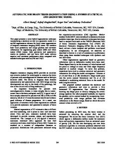
2. ATLAS MATCHING ALGORITHM 2.1. Global atlas registration In [2], we propose an automated procedure to find the best parameters for the 3D second degree global transformation proposed and routinely used by Thurjfell et al. in [1] for registering the Computerized Brain Atlas (CBA, University hospital of Karolinska, Sweden) with an MR image. The registration method is based on the matching of 2 important anatomical landmarks: the cortical surface and the ventricular system. First, the cortical surface of the brain is segmented from the MR image using a directional watershed algorithm proposed in [10] followed by mathematical morphology based operations to simplify the brain surface. Only a coarse cortical surface (without sulci) and the ventricular system will used by the matching criterion (see Figure 1).
Figure 1 : slice of original MR image, segmentation using directional watersheds, extracted cortical surface and ventricles, simplified cortical surface Similarly to [3], we define our registration criterion as a distance measure between this surface Smob and the equivalent reference object in the atlas Sref :
∑
1
d S2ref (x ) 2 x∈S d ( S ref , S mob ) = mob # (S mob ) whith
{
d Sref (x ) = min d (x, y ) | y ∈ S ref
(1)
}
(2)
This distance measure can be efficiently computed by precomputing the distance d S ref (x ) from any pixel x to the reference surface Sref using the Distance Transform algorithm that we describe in [5], which is mainly an efficient implementation of the Euclidean Distance Transform proposed in [4]. True Euclidean distance is indeed required here since its commonly used Chamfer approximations fail to provide a good estimate of the gradient of the distance. The global transformation is then
considered as the linear combination of 30 de-correlated basic transformations whose coefficients are optimized by a steepest gradient minimization of the criterion in the 30-dimensional coefficient space. This global transformation is equivalent to the routinely used transformation performed by the manual registration of the CBA. This part of our algorithm mainly is an automation of this procedure. Improving these results, i.e. providing a correct local shape and not only a correct localization for the brain structures, requires adding complexity to both the possible deformations and the matching criterion. We believe that by exploiting local image information, as well as prior information for visible structures in the image, it is possible to refine these results significantly. Optical flow methods could provide us with an efficient and robust method for matching individual structures on the target scan, but these methods are computationally heavy, and require a multi-resolution scheme to achieve a good accuracy. Also, the reference MR image of the atlas is needed. Since the CBA has been drawn from anatomical brain slices, we only have the contours of the atlas objects. Therefore we have chosen to use active surfaces for the local deformation of the initialized surfaces. 2.2. Active surface model We propose an active surface model to refine the local shape of the globally registered structures. The concept of active contours was first introduced by Kass and al. [6]. They define active contour models as parametric curves v(s) = (x(s),y(s)) where s ∈ [0,1], evolving to minimize an energy typically defined as 1
∫
E (v) = w1 ( s) 0
∂v ∂s
2
+ w2 ( s )
∂ 2v ∂s 2
2
+ P (v( s)) ds
(3)
E is a combination of smoothness terms designed to hold the curve together (elasticity term weighted by w1) and keep it from bending too much (rigidity term weighted by w2) and a third term driving the curve towards the edges of the image. This later term is typically a decreasing function of the gradient of the smoothed image. The minimization of the energy is done locally by solving the corresponding Euler Lagrange equation ∂v( s, t ) ∂ ∂v( s, t ) ∂ 2 ∂ 2 v( s, t ) − w1 + λ∇P(v( s, t ) ) = 0 + 2 w2 ∂t ∂s ∂s ∂s ∂s 2
(4)
To reach a global minimum, the curve needs to be fairly well initialized. This model can be extended to 3D parametric surfaces with two parameters s,r : v(s,r) = (v1(s,r),v2(s,r),v3(s,r)). As proposed by Cohen & al. in [7], the minimization can then be efficiently solved using finite element methods provided we have a meshed description of our surface. The meshing problem will be inspected later. The energy term has been simplified, taking into account only the first order derivatives in the smoothness terms. Hence, the energy is defined as : E (v ) =
∫∫
w10 (r , s)
∂v ( r , s ) ∂r
2
+ w01 (r , s)
∂v ( r , s ) ∂s
2
+ P (v(r , s)) drds
(5)
This energy can then be minimized by solving the corresponding Euler-Lagrange equation : ∂v ∂ ∂v ∂ ∂v − ω10 . − ω 01. = − F (v) ∂ ∂ ∂ ∂ ∂r t s s r v(0, s, r ) = v ( s, r ) (initial estimate) 0
(6)
This equation can be solved using finite element methods. Readers are referred to [11] for complete details about the finite element method. If we discretise the temporal derivative using finite differences, equation (6) becomes :
U t − U t −1 + A.U t = BU t −1 τ
(7)
where U represents the node vector, A the smoothness matrix, B the external forces vector and τ the time step. These equations are efficiently solved using a semi-explicit resolution scheme. 2.3. External forces The external forces, driving the active surface towards the edges of the structure in the image, are computed on each element of the mesh and distributed over the nodes belonging to the element using the element’s shape functions [11]. Classically, the image energy is computed as a decreasing function of the gradient so that it is minimal at the edges of the image. The image force is of course the gradient of the energy. In our case, we have 1 F (v) = ∇(P(v) ) = ∇ 2 1 + (∇I )
(8)
where ∇I is the local smoothed gradient. This expression does not include the sign of the gradient which has therefore been added to the expression of the external force. This prevents both sides of a thin surface from sticking together on the same edge in the image, which is very likely to happen for ribbon-like structures. Also, to prevent several neighboring nodes being displaced towards a spot where the gradient is important, forces are constrained to move along the surface normal direction n only. This requirement also ensures a fairly regular sampling of the surface while it deforms. This yields the following complete expression for the image force : 1 .n .Gexp F (v) = ∇ 2 1 + (∇I )
(9)
where + 1 if Gexp = − 1 if
n .∇I .k > 0 n .∇I .k < 0
(10)
and k=+1 if the region to be segmented has a brighter gray level than the surrounding tissues; k=-1 if the region to be segmented has a darker gray-level than the surrounding tissues. In regions where the gradient is relatively small, where the surface is quite far away from the structure’s edge, the direction of the normal force is computed using precomputed object statistics, shrinking the surface to the edges if it is located outside the object, and expanding if it is inside the object. The force is then defined as : F (v) = + n F (v) = −n
if
I ( v ) − µ ≤ kσ
(curve in the object )
if
I ( v ) − µ ≥ kσ
(curve out of the object )
(11)
where µ is the mean intensity of the target object, σ the standard deviation of the object intensity and k is a user defined constant. In [9], this active surface model has been successively applied for structures exhibiting well-defined features in the image. However, structures that were not initialized close enough to the actual contours in the image sometimes could not be segmented correctly. Therefore, a model of the brain atlas preserving the spatial relationship between neighboring structures is needed.
2.4. Creation of a multi-object surface-based atlas The multi-object model of the CBA atlas has been created from a labeled 3D image where each structure is represented by a given gray-value. This image has been obtained by filling the inside of the contour lines of the atlas’s structures. In order to preserve the spatial relationship between neighboring objects in the atlas, each structure has to share portions of its boundary with its neighboring structures in a well-defined fashion. In [9], we chose to mesh structures individually using a modified Marching Cubes algorithm. If this algorithm were to be applied to generate multi-object meshes where all triangular faces are shared by two structures, the algorithm would generate holes in the cubes where 3 structures intersect. This does not match the requirement of a multi-object mesh. We need a fully connected multi-object mesh. If one decides to mesh the multi-object image using cubic grid points, full connectivity could be ensured but neighboring grid points could share either a face, an edge, or just a corner. These two later cases would obviously generate topological problems for the active surface model. A grid that defines a unique kind of boundary elements between neighboring grid points is the Face Centered Cubic (FCC) grid.
Figure 2 : rhombic dodecahedron In a FCC grid, the voronoi neighborhoods of grid points are rhombic dodecahedra (see figure 2). On figure 2, the neighboring grid points of g are the grid points that are located in the middle of the edges of the wireframe cube (represented only to facilitate visualization) surrounding the rhombic dodecahedron (ni, i=1,2,…,12). Hence, neighboring grid points always share one of the dodecahedron’s faces [8]. This is very convenient for determining a unique kind of boundary elements in a multi-object image. Each face of the dodecahedron is divided into two triangles, whose size can easily be modified either by resampling the FCC grid, or by oversampling or decimating the resulting multi-object mesh. If an FCC grid is relatively coarse, the edges of the structures will appear jagged. To improve the multi-object mesh and remove this jaggedness, the structures’ surfaces are subsequently displaced towards the actual edges of the atlas’s multi-object image with smoothness constraints. Figure 3 shows a multi-object mesh of the sub-cortical brain structures (these are the structures that are surrounded by the ventricles).
Figure 3 : Multi-object mesh of main sub-cortical objects This algorithm provides us with multi-object triangulated surfaces. Each structure has a list of triangles representing its own surface. Each triangle points to the number of the neighboring structure it shares the triangle with.
The surfaces can still be deformed one by one as we did it in our previous work [9]. One way to exploit the data structure that we built around the atlas is to deform all the atlas objects concurrently. This can be done by adding the linking forces between the nodes of neighboring structures to the image force and updating them after each iteration of the energy minimization process. This requires huge amounts of memory and computational power to be solved, and turns out to be highly unstable and difficult to control. Another way one can take advantage of the data structure is to deform the atlas structures sequentially, and subsequently applying the resulting deformation to linked structures. This approach can be very powerful provided this is done in an hierarchical way. 2.5. Hierarchical deformation of the multi-object atlas After the global deformation model has been applied to the multi-object surface based atlas, the local shape of the structures is refined using multi-object active surfaces in a hierarchical way. Structures exhibiting well-defined image features are deformed first, forcing neighboring structures to follow the deformation, while structures with slightly less-well defined features are processed next. The advantage of using the multi-object model is that while individual surfaces deform, the spatial relationship between neighboring structures is preserved. This prevents neighboring structures from intersecting and in this way, structures cannot deform towards edges of structures that were processed previously. The algorithm deforms the structures using the active surface algorithm described in section 2. The weight of the equation’s parameters (smoothing parameter w=w10=w01 and image force parameter) evolve as follows: first the smoothing parameters have a great weight as compared to the image force until a significant number of nodes have reached the edges of the structure (practically, when the gradient associated to these nodes starts to be significant). The relative importance of the smoothing force then decreases gradually to allow the nodes to move without constraints towards the edges in the image. The iterative process is stopped when 80% of the nodes have reached stability. Once a given structure has been deformed, i.e. the Euler-Lagrange equations are solved, the displacement of the structure’s nodes is propagated to the neighboring structures through the multi-object mesh structure. The nodes of previously deformed structures are considered as fixed.
3. RESULTS 3.1. Global registration - sub-cortical brain structures On figure 4, one can observe that the shape of the ventricles differs significantly from the target scan, thereby also causing a shift for structures such as the thalami and the caudate nuclei.
Figure 4 : Axial view of globally registered sub-cortical structures
3.2. Global registration - cortical surface and main sulci Figure 5 presents the matching results of the global transformation for the cortical surface, and for the main sulci. The shape of the cortical surface matches the outer surface very well. Most sulci are very well located, but due to their ribbon-like shape, a slight shift could lead to an incorrect identification.
Figure 5 : Global registration of major sulci and cortical surface This method provides us with an accurate localization of most brain structures, but the transformation is too global to account for local shape differences between the patient and the atlas model. 3.3. Multi-object active surface hierarchical deformation Each slice of the original scan is first filtered using a 3 by 3 median filter to remove the noise and the signal inconsistencies. After that, the image is resampled so as to have cubic voxels. Also, to improve the attraction of the atlas’s structures to the edges in the image, the image is preliminary smoothed. Figure 6 shows the global registration and the subsequent hierarchical deformation of the lateral ventricles and caudate nuclei. If the nuclei had been deformed as single objects, independently from the ventricles, the structure would not have converged towards the actual edges in the image. By deforming the ventricular system first, and propagating this deformation to the nodes it shares with the nuclei, one ensures that the nuclei will be matched correctly. On the images of figure 6, one can also observe the interest of adding the expected gradient sign to the image force. In this case, it has prevented the inner boundary of the right ventricle (on the left hand side in the image) from sticking on the edge of the left ventricle (on the right hand side in the image). For the ventricles, the expected gradient sign in the surface normal direction is negative (dark voxels surrounded by brighter voxels). At the beginning of the surface deformation process, the gradient sign along the surface normal direction is positive at the inner nodes of the interior right ventricle. This causes these nodes of the surface to be displaced towards the left in the image.
Figure 6 : Left : axial view of globally registered caudate nuclei and lateral ventricles Right : same structures after hierarchical deformation
Figure 7 : axial view of thalami, ventricles and putamen Figures 8 and 9 show similar results for a different image on different views. The displayed image is median filtered. One can also notice that, because of the larger ventricles, the deformation of the ventricles is easier to perform.
Figure 8 : Left : coronal view of the globally registered ventricular system and caudate nuclei Right : ventricular system and caudate nuclei after hierarchical deformation
Figure 9 : Left : sagittal view of the globally registered left ventricle and caudate nucleus Right : same structures after hierarchical deformation
Figure 10 : 3D rendering of matched ventricles, caudate nuclei, thalami and putamen with axial, sagittal and coronal cuts through the image
4. CONCLUSION AND PERSPECTIVES We have implemented a hierarchical multi-object surface based deformable model for the automatic localization of brain structures in MR images. Figure 11 recalls the main steps of our algorithm. The framework of the algorithm can be seen as a 3D non-linear correspondent to the philosophy of Kalman filtering in signal processing. We first have a very strong confidence in our model – the CBA database – and then progressively take into account the additional information coming from the data itself. The advantages of this method are manifold. The first advantage is that most global registration methods are rigid-based and use simpler landmarks. The use of a second degree transform instead of a first degree global transform allows the landmarks to be matched more efficiently, providing us with an accurate localization of all structures. Also, the use of the cortical surface as a matching criterion for the global transform provides us with a better localization of most sulci, as compared to usual global registration methods. The multi-object model built from the atlas is useful to preserve the spatial relationship between neighboring structures while the atlas deforms. If the local refinements to be performed are small, the multi-object active surface refinement turns out to be a powerful solution, especially for the sub-cortical brain structures. However, if the patient’s brain has been deformed too much because of a disease for instance, the model does not work well. Structures such as the ventricles will still be segmented correctly, but the transmission of its deformation to the neighboring structures will lack volumetric constraints. The deformation then sometimes generates self-intersecting structures. Therefore, at this point, the algorithm works best with images of healthy patients. To account for more complex deformations, a volumetric model of the brain is needed. For most sulci, the refinements using active surfaces cannot be carried out efficiently because the initialization sometimes is closer to another sulci at some of its nodes, which generates instabilities in the minimization process. We believe that a volumetric deformation model, incorporating the tissue’s characteristics will be a great advantage for the matching process.
Figure 11 : atlas matching scheme For these reasons, our work is now concentrating on the development of a volumetric finite element based deformation model, to be able to identify and segment accurately images of both healthy brains and brains affected by tumors, lesions, expanded ventricles, …
ACKNOWLEDGEMENTS Olivier Cuisenaire and Matthieu Ferrant are working towards a Ph.D. thesis with a grant from the Belgian FRIA (Fonds pour la Formation à la Recherche dans l’Agriculture et l’Industrie).
REFERENCES 1. 2. 3. 4. 5. 6. 7. 8.
L. Thurjfell, C. Bohm, T. Greitz and L. Eriksson. Transformations and algorithms in a Computerized Brain Atlas. IEEE Transactions on Nuclear Sciences. vol. 40. pp. 1187-1191, 1993. O. Cuisenaire, J.P. Thiran, B. Macq, C. Michel, A. De Volder and F. Marques. Automatic registration of 3D MR images with a computerized brain atlas, SPIE Medical Imaging 96, Newport Beach, SPIE vol. 1719, pp. 438-449 J.F Mangin, V. Froin, I. Bloch, B. Bendriem and J. Lopez-Krahe. Fast non-supervised 3D registration of PET and MR Images from the brain. Journal of Cerebral Blood Flow and Mechanism, vol. 14, pp. 749-792, 1994 P.E.Danielsson. Euclidean Distance Mapping, Computer Graphics and Image Processing 14, 1980, 227-248. O. Cuisenaire. Region Growing Euclidean Distance Transforms. ICIAP’97, Florence, September 97, Lecture Notes in Computer Science. M. Kass, A. Witkin and D. Terzopoulos. Snakes, active contour models. International Journal of Computer Vision, vol. 1, pp. 321-331, 1988 L.D. Cohen and I. Cohen. Finite element methods for active contour models and balloons for 2D and 3D images. IEEE Pattern Analysis and Machine Intelligence, 15, November 1993 G.T. Herman and E.Zhao. Jordan Surfaces in Simply Connected Digital Spaces. Journal of Mathematical Imaging and Vision, vol. 6, pp. 121-138, 1996.
9.
O. Cuisenaire, M. Ferrant, J.-Ph. Thiran and B. Macq, Model-based segmentation and recognition of anatomical brain structures in 3D MR Images, NMBIA'98, Glasgow, July 1998. 10. J.-Ph. Thiran, V. Warscotte, B. Macq, A queue-based region growing algorithm for accurate segmentation of multidimensional images, Signal Processing, Vol. 60, 1997, pp. 1-10. 11. O.C. Zienkiewickz and R. L. Taylor, The Finite Element Method. McGraw Hill Book Co., NY, 4th edition, 1987.