Multi-Resource Management in Embedded Real-Time Systems

Multi-Resource Management in Embedded Real-Time Systems

PROEFSCHRIFT

ter verkrijging van de graad van doctor aan de Technische Universiteit Eindhoven, op gezag van de rector magnificus, prof.dr.ir. C.J. van Duijn, voor een commissie aangewezen door het College voor Promoties in het openbaar te verdedigen op woensdag 17 oktober 2012 om 16.00 uur

door Michał Jakub Holenderski

geboren te Warschau, Polen

Dit proefschrift is goedgekeurd door de promotor: prof.dr. J.J. Lukkien Copromotor: dr.ir. R.J. Bril

Printed by: Eindhoven University Press, Eindhoven, The Netherlands © Michał Holenderski 2012

All rights are reserved. Reproduction in whole or in part is prohibited without the written consent of the copyright owner. A catalogue record is available from the Eindhoven University of Technology Library ISBN: 978-90-386-3237-7

Contents 1 Introduction 1.1 Problem statement . . . . . . . . . . . . . . . . . . . . . . . . . . . . . 1.2 Contributions . . . . . . . . . . . . . . . . . . . . . . . . . . . . . . . . 1.3 Outline . . . . . . . . . . . . . . . . . . . . . . . . . . . . . . . . . . .

1 3 3 4

2 System model 2.1 Resource model . . . . . . . . . . . . . . . . . . . . . . . . . . . . . . . 2.2 Application model . . . . . . . . . . . . . . . . . . . . . . . . . . . . . 2.3 Mapping . . . . . . . . . . . . . . . . . . . . . . . . . . . . . . . . . . .

5 5 7 11

3 Processor management 3.1 Related work . . . . . 3.2 System model . . . . . 3.3 RELTEQ . . . . . . . 3.4 Periodic tasks . . . . . 3.5 Servers . . . . . . . . . 3.6 Hierarchical scheduling 3.7 Evalulation . . . . . . 3.8 Discussion . . . . . . .

. . . . . . . .

. . . . . . . .

. . . . . . . .

. . . . . . . .

. . . . . . . .

. . . . . . . .

. . . . . . . .

. . . . . . . .

. . . . . . . .

. . . . . . . .

. . . . . . . .

. . . . . . . .

. . . . . . . .

. . . . . . . .

. . . . . . . .

. . . . . . . .

. . . . . . . .

. . . . . . . .

. . . . . . . .

. . . . . . . .

. . . . . . . .

17 19 24 29 33 35 42 44 50

4 Memory management 4.1 Related work . . . . . . . . . . . . 4.2 System model . . . . . . . . . . . . 4.3 Reducing memory requirements . . 4.4 Handling overload conditions . . . 4.5 Bounding the mode change latency 4.6 Discussion . . . . . . . . . . . . . .

. . . . . .

. . . . . .

. . . . . .

. . . . . .

. . . . . .

. . . . . .

. . . . . .

. . . . . .

. . . . . .

. . . . . .

. . . . . .

. . . . . .

. . . . . .

. . . . . .

. . . . . .

. . . . . .

. . . . . .

. . . . . .

. . . . . .

. . . . . .

55 57 62 68 77 79 93

5 Multi-resource management 5.1 Related work . . . . . . . . . . . . . . . . 5.2 Recap of related synchronization protocols 5.3 Towards multi-resource sharing . . . . . . 5.4 System model . . . . . . . . . . . . . . . . 5.5 Parallel-SRP (PSRP) . . . . . . . . . . . . 5.6 Schedulability analysis for PSRP . . . . . 5.7 Evaluation . . . . . . . . . . . . . . . . . . 5.8 Discussion . . . . . . . . . . . . . . . . . .

. . . . . . . .

. . . . . . . .

. . . . . . . .

. . . . . . . .

. . . . . . . .

. . . . . . . .

. . . . . . . .

. . . . . . . .

. . . . . . . .

. . . . . . . .

. . . . . . . .

. . . . . . . .

. . . . . . . .

. . . . . . . .

. . . . . . . .

. . . . . . . .

95 97 101 106 107 110 113 128 130

. . . . . . . .

. . . . . . . .

. . . . . . . .

. . . . . . . .

. . . . . . . .

. . . . . . . .

6 Grasp 133 6.1 Related work . . . . . . . . . . . . . . . . . . . . . . . . . . . . . . . . 135 i

ii

CONTENTS 6.2 6.3 6.4 6.5 6.6

Grasp overview . . . . . . . . . . . . . Multiprocessor scheduling . . . . . . . Hierarchical scheduling . . . . . . . . . Hierarchical multiprocessor scheduling Timestamp synchronization . . . . . .

. . . . .

. . . . .

. . . . .

. . . . .

. . . . .

. . . . .

. . . . .

. . . . .

. . . . .

. . . . .

. . . . .

. . . . .

. . . . .

. . . . .

. . . . .

. . . . .

. . . . .

. . . . .

136 141 144 146 147

7 Conclusion

151

Bibliography

153

Symbol index

164

Acronyms

166

Accomplishments

167

Summary

171

Curriculum Vitae

174

Chapter 1

Introduction The history of the modern computer starts in 1944 with the Colossus. It was the world’s first electronic, digital programmable computer, used by the British to decrypt German messages during World War II. It used vacuum tubes instead of mechanical or electrical relay switches found in its predecessors. The vacuum tubes were the computational units and were interconnected by simple copper wires. The machine was programmed by manually routing the wires. The first general-purpose electronic computer was the ENIAC, completed in 1946. Like the Colossus, it was colossal, weighing 30 tons, occupying 165 m2 , and consuming 174kW of power (McCartney, 1999). Its 18 000 vacuum tubes could perform 5000 additions per second, and were initially used by the US army for computing the behavior of chemical reactions inside of a hydrogen bomb for the Manhattan project and later for ballistic analysis. The invention of the transistor and the integrated circuit in the late 1940s, followed by their mass production in the 1950s, made it possible to shrink computers and to reduce their cost, making them available for many new applications. Initially they found their application in large and powerful mainframe computers, where several users at a time could execute their computations on a shared mainframe computer. With their ever shrinking size, however, digital computers could also be used for controlling smaller systems. A prominent example is the Apollo Guidance Computer, which was responsible for guidance, navigation and control of the Apollo spacecrafts on their lunar missions in the late 1960s. It weighed 32kg, occupied 1 cubic foot, had 2K of RAM, and 36K of hard-wired core-rope memory with copper wires threaded or not threaded through tiny magnetic cores. It consumed 55 Watts and could perform 40 000 additions per second (O’Brien, 2010). The state of the art in scheduling in those days was to divide the entire control application into individual tasks, and to schedule them according to a round robin, First-In-First-Out, or table driven scheme. However, the safety critical nature of the Apollo Guidance Computer, combined with its limited resources, required new task scheduling methods, giving rise to one of the earliest priority-based schedulers. In the case of an overload, the scheduler would continue executing the highest priority tasks, at the cost of dropping those with a 1

2

Introduction

lower priority (Martin, 1994). As digital computers were increasingly used for controlling safety critical systems, theories for reasoning about the behavior of these systems started to emerge, in particular, the real-time scheduling theory. Its goal is to analyze the mapping of the digital resources (such as the processor, memory or network) to tasks to ensure that the tasks’ timing constraints (derived from the system timing constraints) are met. The seminal paper by Liu and Layland (1973) is often regarded as the beginning of the real-time scheduling theory. It proposed sufficient and necessary utilization bounds for fixed priority preemptive scheduling on uniprocessor systems. Since then, real-time theory has addressed more complicated systems, such as multiprocessor and distributed platforms, with dependencies between tasks, and various other constraints. Even though significant progress has been made, real-time scheduling and analysis still o↵ers many challenging and fundamental open problems, in particular in the multiprocessor domain (Davis and Burns, 2011). The Apollo Guidance Computer can be regarded as the precursor of modern embedded systems. Unlike large super computers, embedded devices have stringent operational constraints, such as weight, size, and cost. Consequently, embedded systems are characterized by limited processing, storage and energy resources. For example, due to the weight constraints, an airplane will reuse the same computer hardware to run the control software during di↵erent modes of operation, such as takeo↵, flight, and landing. Switching between the di↵erent modes of operation must be efficient and predictable, without disturbing the operation of the entire system. It is often too costly to develop dedicated hardware for solving a particular problem, which has lead to a wide adoption of general purpose computers, exemplified already by the Colossus vs. ENIAC. General purpose computers o↵er the flexibility to reuse the same hardware for di↵erent applications. As computer platforms and applications become ever more complex, however, the programmers must rely on operating systems providing higher level abstractions for managing the resources. In embedded systems this is often achieved by explicit fine-grained multi-resource management of the various resources comprising the platform. A popular abstraction are resource reservations (Mercer et al., 1994), which aim at providing temporal isolation between independent tasks. They form the basis for virtual platforms, which provide tasks with the illusion of executing on a dedicated platform, often comprised of several di↵erent resources. As applications became increasing complex, comprised of hundreds of tasks, it became more difficult and costly to develop large systems. This gave rise to componentbased engineering, which o↵ers a modular approach for designing and developing complex systems by grouping the tasks performing a particular function inside of components. Several component models for real-time systems were proposed since, most notably the periodic resource model (Shin and Lee, 2003), aiming to facilitate independent development and analysis of components. Hierarchical scheduling is then used to schedule components on the global level, and tasks locally within components. Due to the limited resources in embedded systems, it is important that the mechanisms provided by an operating system, such as task scheduling and timer management, are efficient and introduce little overhead.

Problem statement

3

We conducted our work within the context of multimedia processing systems in the surveillance domain. The hardware platforms in this domain are usually resourceconstrained embedded systems, comprised of multiple di↵erent resources, such as a processor, memory and digital signal processors. The multimedia applications which are mapped to these platforms have real-time constraints, are data intensive, and experience high variability of resource requirements due to data-dependent workload. For example, an MPEG encoder will require more processing time for a scene with a lot of movement. Consequently, the encoded video frames will vary in size, requiring variable amount of network bandwidth during transmission and memory during decoding. If several video streams are processed on the same platform, and their total resource requirements exceed the available resources, then a tradeo↵ needs to be maintained between the resource requirements and the quality of the individual streams (expressed in terms of e.g. timing constraints on individual frames), to guarantee a system wide quality of service. We considered multimedia processing applications comprised of several scalable components, which can operate in di↵erent modes and are scheduled by a hierarchical scheduling framework.

1.1

Problem statement

This thesis addresses the problem of mapping multiple heterogenous resources to tasks in the context of resource constrained embedded real-time systems. It focuses on three research questions: 1. How can we design an efficient hierarchical scheduling framework for supporting independent development and analysis of component based systems, to provide temporal isolation between components? 2. How do we change the mapping of resources to tasks and components during run-time efficiently and predictably, and how do we analyze the latency of such a system mode change in systems comprised of several scalable components? 3. How do we schedule and analyze a set of parallel-tasks which require simultaneous access to several di↵erent resources, while guaranteeing that all tasks meet their deadlines?

1.2

Contributions

In Chapter 2 we propose a system model, comprised of a resource model, an application model, and a mapping between the two. The novel resource model abstracts the key properties of heterogenous resources from a scheduling perspective, providing a uniform model for di↵erent resources, such as a processor, memory or network. The application model is based on the notions of tasks and components, and supports the modeling and analysis of hierarchical and reservation-based systems.

4

Introduction

In Chapter 3 we present RELTEQ, which is a general timer management system exhibiting low processor and memory overheads. We then leverage RELTEQ to design and implement an efficient hierarchical scheduling framework, which provides temporal isolation between components. The system overheads are evaluated based on an implementation within µC/OS-II, a real-time operating system used in the industry in various domains, such as aerospace, automotive, medical, and surveillance. In Chapter 4 we investigate scalable applications operating in a memory-constrained system. A scalable application, comprised of scalable components, can operate in one of several predefined system modes, defined in terms of component modes. A component mode defines a trade-o↵ between its resource requirements and its output quality. During runtime the system may reallocate the resources between the components, resulting in a system mode change. The latency of a system mode change, defined as the time duration between a mode change request and the time that it has been e↵ected, should satisfy an upper bound. We first show how to reduce the memory requirements in a streaming multimedia application. We then show how to provide guaranteed resource access in spite of mode changes, while at the same time minimizing the mode change latency bound. We present a novel mode change protocol called Swift Mode Changes, which relies on fixed priority with deferred preemption scheduling. The design, analysis and implementation are presented and evaluated based on a quantitative analysis. In Chapter 5 we address the problem of scheduling periodic parallel tasks on a multi-resource platform, where tasks have real-time constraints. The goal is to exploit the inherent parallelism of a platform comprised of multiple heterogeneous resources. A new scheduling algorithm called PSRP is presented, together with the accompanying schedulability analysis. The benefits of PSRP are demonstrated by means of simulation results and an example application showing that PSRP indeed exploits the available concurrency in heterogeneous real-time systems. In Chapter 6 we present a trace visualization toolset called Grasp, which we have used extensively during the design and development of the various real-time operating system extensions described in this thesis. It provides and clear and intuitive user interface and a simple architecture, making it easy to extend Grasp with new visualizations.

1.3

Outline

This thesis is structured as follows. Chapter 2 introduces the system model, which is used later in Chapters 3, 4, and 5. Each of these chapters instantiates and extends the model for its particular needs. Chapters 3, 4, 5, and 6 discuss the main contributions outlined in Section 1.2. Chapter 7 concludes this thesis. A list of publications contributing to this thesis can be found in the Accomplishments appendix.

Chapter 2

System model A system consists of applications, resources and a mapping between them. Application workload is expressed in terms of tasks, where a task represents the work which needs to be done in response to an event, such as processing a newly arrived video frame. The mapping of resources to tasks describes how the “ownership” of resources changes during runtime, i.e. which task “owns” a particular resource at a particular time. The ownership may change, e.g. if several tasks need to access the same memory region or the same processor. A mapping must satisfy certain soundness constraints, e.g. every mutually exclusive resource is owned by at most one task at a time. In real-time systems there are additional timeliness constraints, which are often expressed in terms of task deadlines. Embedded systems exhibit additional constraints which address the overheads associated with the mapping due to limited resources, such as scheduling, and context switching overheads. In this chapter we present an abstraction which allows us to model the scheduling of tasks on di↵erent resources in a uniform way. The essential abstraction is that any resource (such as a processor, memory space or bus) can be represented as a multi-unit preemptive or non-preemptive resource.

2.1

Resource model

The purpose of a resource model is to provide a certain level of abstraction helping to describe the mapping of physical resources to tasks. It has to be simple enough to reason about, while at the same time expressive enough to use the available resources efficiently. The main contribution of our model is the ability to schedule tasks on various di↵erent resources, such as processor and memory, in a uniform way. At the core of our resource model is the multi-unit resource. Definition 2.1 (Multi-unit resource). Let R be the set of all resources in the system. A multi-unit resource r 2 R consists of multiple units, where each unit is a serially accessible entity. A resource r is specified by its capacity Nr 1, which represents the maximum number of units the resource can provide simultaneously. 5

6

System model

Memory space is an example of a multi-unit resource. In this thesis, when talking about the memory space resource we are interested in the memory requirements in terms of memory size, and ignore the specifics of memory allocation and the actual data stored in the memory. A memory, managed as a collection of fixed sized blocks, can be regarded as a multi-unit resource with capacity equal to the number of blocks. In this sense our multi-unit resource is similar to a multi-unit resource discussed by Baker (1991). The capacity of a multi-unit resource represents essentially the maximum number of tasks which can use the resource simultaneously. A multi-core processor can therefore be modeled as a resource with capacity equal to the number of cores. Resource management is about managing access to scarce resources, i.e. resources for which at times the demand may exceed their provision. If the total requirement for a resource never exceeds its capacity, then the management is trivial: we can always provide access to the resources. When modeling systems we can therefore ignore resources for which the demand never exceeds their provision. Single-unit resources are a special case of multi-unit resources. Definition 2.2 (Single-unit resource). A single-unit resource r 2 R is a multi-unit resource such that Nr = 1 A single-core processor is an example of a single-unit resource, since only a single task can be using it at a time. A memory controller synchronizing the access to a memory space can also be regarded as a single-unit resource1 . In the remainder of the thesis we assume multi-unit resources with capacity greater than 1, unless explicitly stated otherwise.

2.1.1

Preemptive vs. non-preemptive resources

A preemption is the change of ownership of a resource unit before the owner is ready to relinquish the ownership. In terms of the traditional task model, a job (representing the ownership of a resource) may be preempted by another job before it completes. We can classify all resources in one of two categories: Definition 2.3 (Preemptive resource). The usage (or ownership) of a unit of a preemptive resource can be preempted without corrupting the state of the resource. We use P ✓ R to denote the set of all preemptive resources in the system. Definition 2.4 (Non-preemptive resource). The usage (or ownership) of a unit of a non-preemptive resource may not be preempted without the risk of corrupting the state of the resource. We use N ✓ R to denote the set of all non-preemptive resources in the system. Every resource is either preemptive or non-preemptive, i.e. (N [ P = R) ^ (N \ P = ;).

(2.1)

1 A memory can therefore be modeled by two resources: one representing the memory space and the other representing mutually exclusive access to the memory.

Application model

7

A processor is an example of a preemptive resource, as the processor state of a running task can be saved upon a preemption and later restored. A bus is an example of a non-preemptive resource, as an ongoing message transfer cannot be preempted without loosing the message. A logical resource (e.g. a shared variable) is another example of a non-preemptive resource. Preemption is usually provided on the software level, by the operating system. For example, when an interrupt arrives, the operating system first stores the processor state, then executes the interrupt handler, and finally restores the saved processor state. Note that actually the usage of nearly any resource can be preempted: e.g. memory space (usually considered a non-preemptive resource) can be “switched out” to a memory higher in the memory hierarchy (e.g. data can be moved from the processor cache to the RAM), or the data can be simply overwritten and recomputed later. However, this will come at the cost of a performance penalty (incurred by storing-and-restoring or recomputing the state of the resource). A non-preemptive resource is basically one for which the system designer has decided that its preemption overhead is too large. We assume mutually exclusive access to resources, meaning that each unit of a multi-unit resource can be accessed by at most one task at a time. For example, each core in a multicore processor can be accessed by at most one task at a time. Notice that preemptiveness is orthogonal to mutual exclusion, as mutual exclusion holds for both preemptive and non-preemptive resources.

2.1.2

Physical vs. virtual resources

Physical resources are the hardware resources provided by the platform, such as a processor, memory or bus. As we will see later in Section 2.2.2, application components can provide their own virtual resources. We use R to denote both physical and virtual resources. Similar to physical resources, each virtual resource is either preemptive or non-preemptive.

2.2

Application model

Let T = R+ 0 be the time domain (of non-negative real numbers), with t 2 T representing a time instant or the duration of a time interval.

2.2.1

Tasks

We model applications in terms of a set of tasks. Each task specifies the resource requirements which are required to do a particular work. Definition 2.5 (Task). A task ⌧i is specified by its • fixed and unique priority ⇡i (lower number indicating higher priority), • period Ti , which specifies the inter-arrival time between two consecutive instances of ⌧i ,

8

System model • initial o↵set (or phasing) Oi , which specifies the arrival time of the first instance of ⌧i , • relative deadline Di , with Di  Ti , • sequence of segments Si , where the j-th segment ⌧i,j 2 Si is specified by its worst-case execution time Ei,j , and a set of resource requirements Ri,j . Each resource requirement (r, n) 2 Ri,j represents a requirement for n > 0 units of resource r 2 R.

We use to denote the set of all tasks in the system, and S to denote the set of all segments in the system, i.e. [ S= Si ⌧i 2

Our task therefore models programs which can be expressed as a sequence of segments, where each segment ⌧i,j is wrapped between a lock (Ri,j ) and unlock (Ri,j ) operation. The semantics of these operations is similar to the primitives used in (Havender, 1968) for locking resources collectively. Priorities are used for resolving conflicts during runtime when more than one task tries to access a shared resource. All segments ⌧i,j 2 Si share its priority ⇡i . We use ⇡? to denote a priority lower than the lowest priority, and ⇡> to denote a priority higher than the highest priority among all tasks. Notation To keep the notation short, if a segment ⌧i,j requires only single-unit resources, or if the number of required units is not important, we will write Ri,j = {r1 , r2 , r3 } instead of Ri,j = {(r1 , 1), (r2 , 1), (r3 , 1)}. We use a shorthand notation to refer to the resources which are required by a segment, where r 2 Ri,j means that 9(x, n) 2 Ri,j : x = r. When specifying segments we use a shorthand notation, where (e, {r1 , r2 , . . .}) represents a segment ⌧i,j with Ei,j = e and Ri,j = {r1 , r2 , . . .}. When applying set operations to sets of resource requirements we are usually interested only in the identity of the resources (and not the number of units). Therefore, for simplicity, we will use Ri,j \ Rx,y to denote {r | (r, n) 2 Ri,j ^ (r, m) 2 Rx,y }, and Ri,j [ Rx,y to Pdenote {r | (r, n) 2 Ri,j _ (r, m) 2 Rx,y }. We use Ei = ⌧i,j 2Si Ei,j to denote the worst-case execution time of task ⌧i . Example 2.1. Our model distinguishes between 2 single-core processors (modeled as 2 single-unit resources) and a single 2-core processor (modeled as one multi-unit resource). In the 2 single-core processors case, we can specify a task requiring simultaneous access for t time units to particular single-core processors, e.g. P = {p1 , p2 }, Np1 = 1, Np2 = 1,

= {⌧1 }, S1

= h(t, {p1 , p2 })i.

In the 2-core processor case we can only specify a task requiring simultaneous access for t time units to a particular number of cores, e.g.

Application model

9

P = {p}, Np = 2,

2.2.2

= {⌧1 }, S1

= h(t, {(p, 2)})i.

Components

Next to the notion of physical resources (described in Section 2.1.2) we introduce the notion of virtual resources, which are provided by components. Definition 2.6 (Component). A component c is specified by its • fixed and unique priority ⇡c (lower number indicating higher priority), • period Tc , which specifies the inter-arrival time between two consecutive instances (or replenishments of the budget) of c, • initial o↵set (or phasing) Oc , which specifies the arrival time of the first instance (or replenishment of the budget) of c, • relative deadline Dc , with Dc  Tc , • set of resource requirements Rc , where each resource requirement (r, n) 2 Rc represents a requirement for n > 0 units of resource r 2 R, • set of resource provisions Pc , where each resource provision (r, n) 2 Pc represents a provision of n > 0 units of resource r 2 R, • time capacity (or budget) Ec , which specifies the amount of time during each period that component c will provide the resources in Pc , while requiring the resources in Rc . We use C to denote the set of all components in the system. A component c provides virtual resources, which are specified in Pc . We include these resources in the set of all resources in the system, i.e. 8c 2 C : Pc ✓ R. The following two examples demonstrate how to express a processor server and a memory bu↵er in terms of our component model. Example 2.2 (A processor server component). A single core processor can be modeled as a preemptive resource cpu 2 P with Ncpu = 1. A processor server s provides a share of a processor bandwidth, which is specified by its replenishment period ⇧s and capacity ⇥s (Shin and Lee, 2003). When a server is running, every time unit its remaining budget is decremented by one. Every ⇧s time units its remaining budget is replenished to ⇥s . In systems with global fixed-priority scheduling each server also has a fixed priority ⇡s .

10

System model

A server s providing a share of processor cpu, can be modeled as a component c 2 C with ⇡c Tc Oc Dc Ec Rc Pc

= = = = = = =

⇡s ⇧s 0 ⇧s ⇥s {(cpu, 1)} {(cpus , 1)}

(2.2)

with cpus 2 P. Example 2.3 (A memory bu↵er component). A memory containing M bytes can be modeled by a non-preemptive resource mem 2 N with Nmem = M . A memory bu↵er component manages a part of the memory space in terms of bu↵er elements and provides a FIFO access to these elements. Each bu↵er q has a finite capacity N umElemsq , defining the maximum number of elements which can be stored in the bu↵er, where each element has a fixed size of ElemSizeq bytes. A bu↵er q, which resides in memory mem and is created during the initialization of the system and never destroyed, can be modeled as a component c 2 C with Tc Oc Dc Ec Rc Pc

= = = = = =

1 0 1 1 {(mem, ElemSizeq ⇤ N umElemsq )} {(elementsq , N umElemsq ), (mutexq , 1)}

(2.3)

with elementsq , mutexq 2 N. Tc = 1 means that the component is aperiodic. Oc = 0 and Dc = Ec = 1 mean that the bu↵er will be created at the system initialization and live until the system terminates. During that time it will require ElemSizeq ⇤ N umElemsq units of the mem resource, and in return it will provide a virtual elementsq resource containing N umElemsq bu↵er elements. A bu↵er provides interface methods to store and retrieve elements from the bu↵er. These methods manipulate the bu↵er’s internal data structures and have to execute in a mutually exclusive fashion. A common implementation will guard these methods with a mutex. A call to the bu↵er’s interface methods is modeled by a requirement for one unit of the virtual mutexq resource for the duration of the call. Since Nmutexq = 1 and mutexq 2 N, only one task may access the bu↵er’s interface methods at a time. Note that a bu↵er requires mutually exclusive access only to its internal data structures. This means that one task can be reading from the bu↵er’s head element, while another task is writing to the tail element, provided that the internal data structures keeping track of the pointers to the head and tail are updated in a mutually exclusive manner. Note that since bu↵ers live in the memory for the entire duration of the system execution, during runtime there is no need for arbitration between two bu↵ers com-

Mapping

11

peting for memory: all bu↵ers need to fit in the memory or the application cannot start executing. Hence, the priority of the bu↵er component is irrelevant.

2.2.3

Applications

We can group tasks and components which together perform a particular function to form an application. Definition 2.7. An application a is specified by its • task set

a

✓ ,

• component set Ca ✓ C. We use A to denote the set of all applications in our system. Every task (or component) belongs to at most one application. We assume that applications are independent and do not share tasks (or components), i.e. 8a, b 2 A : a 6= b ) (

2.3

a

\

b

= ; ^ Ca \ Cb = ;).

(2.4)

Mapping

In Sections 2.1 and 2.2 we have defined the static models describing the resources and the applications. Now we move on to the mapping of resources to applications. The mapping is responsible for time sharing the access to resources during runtime, and is defined by allocation and scheduling. An allocation assigns task segments and components to their required resources, while a schedule describes when segments and components gain access to their assigned resources.

2.3.1

Allocation

In this thesis we assume static allocation of resources (also referred to as partitioning), which is specified in our system model by the resource requirements of task segments and components. In embedded systems, where hardware platforms are usually comprised of several di↵erent resources (e.g. CPU, DSP, DMA controller), tasks must be explicitly mapped to the various resources. In such systems static allocation of tasks to resources is often desired. It also simplifies the scheduling of the entire platform during runtime, since the decision of allocation has been taken o✏ine. Resource identity in multi-unit resources When a task or component requests memory space for storing its data, it assumes that no other task or component will modify and corrupt the data inside of its memory space. This suggests that two parameters should be associated with each granted memory request: its size and its identity. The scheduling function makes sure that a resource request for n units of a multi-unit resource is granted only if the resource

12

System model

has at least n units available. When a request is granted, the requesting task or component has complete control over these units. Protection mechanisms preventing tasks and components from corrupting each others resources are outside the scope of this model. However, when a task or component accessing a resource is preempted it may be critical that it is later resumed on the same resource units. For example, when a job is preempted while it is writing to a particular memory location, once it is resumed it should continue writing to the same location. Our model abstracts from the identity of individual units in a multi-unit resource and therefore it cannot be used to reason about particular resource units. However, we can assume the context switch to be responsible for making sure that a segment is resumed on the appropriate resource units. In the example of a preemption of a task writing to memory, upon preemption the system may store the partially written data to the disk and later restore it to the memory upon resuming.

2.3.2

Scheduling

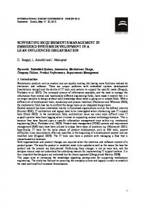
The schedule needs to maintain the timing constraints of tasks and components and mutually exclusive access to shared resources. All these constraints can be resolved o✏ine, giving rise to a time-driven schedule. Alternatively, the scheduling can be done online, where scheduling decisions are event-driven and performed according to a predefined scheduling policy. In this thesis we consider the latter, focusing on FixedPriority Preemptive Scheduling (FPPS) and Fixed-Priority with Deferred-preemption Scheduling (FPDS). We can schedule both tasks and components. When a task segment (or a component) is scheduled on a resource during runtime, we say that the segment (or component) is using the resource, or that it owns the resource. The ownership of a resource may change. However, at any point in time each unit of a multi-unit resource may be used by at most one segment (or component). The scheduling of segments on a multi-unit resource r can be visualized by means of Nr “tracks”, where each track represents the usage of a single unit of resource r, as illustrated in Example 2.4. Example 2.4. Figure 2.1 represents a schedule of segments b, c, and d on resources cpu and dsp, with b scheduled at time 0, d scheduled at time 1 and c scheduled at time 5 and preempting segment d. The arrival pattern of a segment is determined by the task it belongs to, which is discussed in the next section. A resource manages its units internally, meaning that we cannot specify a requirement for a particular unit of a multi-unit resource. A segment can only specify a requirement for a certain number of arbitrary units within a multi-unit resource. However, we assume that while a segment is “executing” on a resource unit the segment will not be migrated to another unit. For example, in Figure 2.1, once d’s requirement for 2 cores of the cpu is granted, d will own the same cpu cores throughout its execution in the time interval [1, 5). Note that the cpu resource may decide to migrate d to di↵erent units when it is preempted at time 5.

Mapping

13 c

cpu.4 cpu.3

d

c

d

cpu.2

d

c

d

cpu.1

b

dsp

b

0

5

10

15

20

25

Figure 2.1: Example of a mapping of segments S = {b, c, d} with Eb = 20, Rb = {(cpu, 1), (dsp, 1)}, Ec = 8, Rc = {(cpu, 3)}, Ed = 7, Rd = {(cpu, 2)}, on a platform containing a 4-core cpu and a single dsp, i.e. R = {cpu, dsp} with Ncpu = 4, Ndsp = 1. We use a dot notation to refer to the individual units in a multi-unit resource. Scheduling of tasks Definition 2.8 (Task schedule). A schedule S : T ⇥ S ⇥ R ! N expresses resource ownership by task segments during runtime, where S (t, s, r) is the number of units of resource r which are owned by segment s at time t. Saying that “at time t segment s owns n units of resource r” is synonymous to saying that “at time t segment s executes on n units of resource r” or that “at time t segment s is scheduled on n units of resource r”. Definition 2.9. We define ⌘ S : T ⇥ S ⇥ R ! {0, 1}, where ⌘ S (t, s, r) returns 1 if at time t segment s is scheduled on resource r, and 0 otherwise, i.e. ( 1 if S (t, s, r) > 0, S ⌘ (t, s, r) = (2.5) 0 otherwise. The scheduling function

S

must satisfy the following criteria:

1. A segment is scheduled only on resources which it requires, i.e. 8t 2 T, s 2 S, r 2 R :

S

(t, s, r) > 0 ) r 2 Rs .

(2.6)

2. A segment is scheduled on all of its required resources, or not at all, i.e. 8t 2 T, s 2 S : (9r 2 Rs :

S

(t, s, r) > 0) ) (8(r, n) 2 Rs :

S

(t, s, r) = n). (2.7)

3. The scheduling function must satisfy the realtime constraints, by making sure that every segment receives its worst-case execution time on its required resources before its parent task’s deadline, i.e. Z k⇤Ti +Di 8k 2 N, ⌧i,j 2 S, r 2 Ri,j : (k + 1)Ei,j  ⌘ S (x, ⌧i,j , r)dx. (2.8) 0

14

System model

Scheduling of components Definition 2.10 (Component schedule). A schedule C : T ⇥ C ⇥ R ! N expresses resource ownership by components during runtime, where C (t, c, r) is the number of units of resource r which are owned by component c at time t. Saying that “at time t component c owns n units of resource r” is synonymous to saying that “at time t component c executes on n units of resource r” or that “at time t component c is scheduled on n units of resource r”. Definition 2.11. We define ⌘ C : T ⇥ C ⇥ R ! {0, 1}, where ⌘ C (t, c, r) returns 1 if at time t component c is scheduled on resource r, and 0 otherwise, i.e. ( 1 if C (t, c, r) > 0, ⌘ C (t, c, r) = (2.9) 0 otherwise. Definition 2.12. We define : T ⇥ C ! T , which captures the remaining budget (or time) of components during runtime, where (t, c) is the remaining budget of component c at time t. The scheduling function

C


4. A component is scheduled only on resources which it requires, i.e. 8t 2 T, c 2 C, r 2 R :

C

(t, c, r) > 0 ) r 2 Rc .

(2.10)

5. A component is scheduled on all of its required resources, or not at all, i.e. 8t 2 T, c 2 C : (9r 2 Rc :

C

(t, c, r) > 0) ) (8(r, n) 2 Rc :

C

(t, c, r) = n). (2.11)

6. The scheduling function must satisfy the realtime constraints, by making sure that every component receives its required time capacity on its required resources before its deadline. The exact specification may di↵er for di↵erent components. For the periodic-idling server component (see Section 3.2.2), the real-time requirement can be formalized as 8k 2 N, c 2 C, r 2 Rc : (k + 1)Ec =

Z

k⇤Tc +Dc

⌘ C (x, c, r)dx.

(2.12)

0

7. Only components with remaining budget are scheduled, i.e. 8t 2 T , c 2 C : (9r 2 R :

C

(t, c, r) > 0) ) (t, c) > 0.

(2.13)

8. The remaining budget should never exceed component’s time capacity, i.e. 8t 2 T , c 2 C : 0  (t, c)  Ec .

(2.14)

Mapping

15

9. The remaining budget of a component c is replenished periodically, with period Tc . Each budget is consumed at a uniform rate whenever it is scheduled. The exact specification may di↵er for di↵erent components. For the periodic-idling server component (see Section 3.1.2), the periodic replenishment and uniform consumption requirement can be formalized as Z t 8k 2 N, c 2 C, t 2 [kTc , (k + 1)Tc ), r 2 Rc : (t, c) = Ec ⌘ C (x, c, r)dx. kTc

(2.15)

Scheduling of tasks and components The scheduling functions

S

and

C


10. The scheduling functions never schedule more units than a resource can provide, i.e. X X S C 8t 2 T , r 2 R : (t, s, r) + (t, c, r)  Nr . (2.16) s2S

c2C

Note that several segments and component may be scheduled on a resource at the same time, as long as together they do not require more units than the resource can provide. 11. A task or component is scheduled on a virtual resource provided by another component only when that component is itself scheduled on its required resources, i.e. 8t 2 T , s 2 S, c 2 C, p 2 Pc : 8t 2 T , c1 , c2 2 C, p 2 Pc2 :

C

S

(t, s, p) > 0 ) (8q 2 Rc :

(t, c1 , p) > 0 ) (8q 2 Rc2

C

(t, c, q) > 0) (2.17) : C (t, c2 , q) > 0) (2.18)

16

System model

Chapter 3

Processor management Modern real-time systems have become exceedingly complex. A typical car is controlled by over 100 million lines of code executing on close to 100 Electronic Control Units (ECU). With more and more functions being implemented in software, the traditional approach of implementing each function (such as engine control, ABS, windows control) on a dedicated ECU is no longer viable, due to increased manufacturing costs, weight, power consumption, and decreased reliability and serviceability (Nolte et al., 2009). With the ECUs having increasingly more processing power, it has become feasible to integrate several functions on a single ECU. However, this introduces the challenge of supporting independent and concurrent development and analysis of individual functions which are later to be integrated on a shared platform. A popular approach in the industry and literature is component-based engineering, where the complete system is divided into smaller software components which can be developed independently. The Automotive Open System Architecture (AUTOSAR) (AUTOSAR, 2011) standard is an example of such an approach in the automotive domain. It relies on a formal specification of component interfaces to verify the functional properties of their composition. Many functions in automotive systems, however, also have real-time constraints, meaning that their correct behavior is not only dependent on their functional correctness but also their temporal correctness. AUTOSAR does not provide temporal isolation between components. Verifying the temporal properties of an integrated system requires complete knowledge of all functions comprising the components mapped to the same ECU, and therefore violates the requirement for independent development and analysis. In this chapter we address the problem of providing temporal isolation to components in an integrated system. Ideally, temporal isolation allows to develop and verify the components independently (and concurrently), and then to seamlessly integrate them into a system which is functioning correctly from both a functional and timing perspective (Shin and Lee, 2008; Nolte, 2011). The question is how to provide true temporal isolation when components execute on a shared processor. We address this problem by means of an hierarchical scheduling framework (HSF). An HSF provides the means for the integration of independently developed and 17

18

Processor management

analyzed components into a predictable real-time system. A component is defined by a set of tasks, a local scheduler and a server, which defines the component’s time budget (i.e. its share of the processing time) and its replenishment policy.

Problem description An HSF-enabled platform should provide the following general functionalities: 1. Interface for the creation of servers and assigning tasks to servers. 2. Virtual timers, which are relative to a components’s budget consumption, as well as global timers, which are relative to a fixed point in time. 3. Local scheduling of tasks within a component, and global scheduling of components on the system level. In this chapter we focus on providing temporal isolation and preventing interference between components. We aim at satisfying the following additional requirement: 4. Expiration of events local to a component, such as the arrival of periodic tasks, should not interfere with other components. In particular, the handling of the events local to inactive components should be deferred until the corresponding component is activated. The time required to handle them should be accounted to the corresponding component, rather than the currently active one. These requirements should be met by a modular and extensible design, with low performance overhead and minimal modifications to the underlying RTOS. It should exhibit predictable overhead, while remaining efficient to support resourceconstrained embedded systems in the automotive domain. Real-time applications will often require support for periodic task arrival. Periodic tasks rely on timers to represent their arrival time. For servers, we also need timers representing the replenishment and depletion of a budget. Vital, and a starting point for our design, is therefore the support for simple timers (or timed events), i.e. the assumption that an event can be set to arrive at a certain time. This simple timer support is typically available in an o↵-the-shelf Real-Time Operating System (RTOS) (Labrosse, 2002). Some RTOSes provide much more functionality (for which our work then provides an efficient realization) but other systems provide just that. As a result, the emphasis lies with the management of timers. The timer management should support long event inter-arrival times and long lifetime of the system at a low overhead.

Contributions We first present the design of a general timer management system, which is based on Relative Timed Event Queues (RELTEQ), an efficient timer management system targeted at embedded systems. Pending timers are stored in a queue sorted on the expiration time, where the expiration time of each timer is stored relative to the

Related work

19

previous timer in the queue. This representation makes it possible to reduce the memory requirements for storing the expiration times, making it ideal for resource constrained embedded systems. We have implemented RELTEQ within µC/OS-II, and showed that it also reduces the processor overhead compared to the existing timer implementation. We then leverage RELTEQ to implement periodic tasks and design an efficient HSF. The proposed HSF extension of RELTEQ supports various servers (including the polling, idling-periodic, deferrable and constant-bandwidth servers), and provides access to both virtual and global timers. It supports independent development of components by separating the global and local scheduling, and allowing each server to define a dedicated scheduler. The HSF design provides a mechanism for tasks to monitor their server’s remaining budget, and addresses the system overheads inherent to an HSF implementation. It provides temporal isolation and limits the interference of inactive servers on the system level. Moreover, it avoids recalculating the expiration of virtual events upon every server switch and thus reduces the worst-case scheduler overhead. The proposed design is evaluated based on an implementation within µC/OS-II, a commercial operating system used in the automotive domain. The results demonstrate low overheads of the design and minimal interference between the components. In this chapter we focus on the means for implementing a HSF. The corresponding analysis falls outside of the scope.

Publications We have introduced RELTEQ in (Holenderski et al., 2009c). In (Holenderski et al., 2010a, 2012a) we have presented an HSF extension of RELTEQ supporting fixedpriority servers. We have extended the design with the constant bandwidth server in (van den Heuvel et al., 2011), and applied it to priority processing in multimedia systems.

3.1

Related work

In this section we summarize the existing work related to the processor management discussed in this chapter.

3.1.1

Processor reservations

Resource reservations have been introduced by (Mercer et al., 1994), aiming at providing temporal isolation for individual components comprising a real-time system, to guarantee resource provisions in a system with dynamically changing resource requirements. They focused on the processor and specified the reservation budget by a tuple (C, T ), with capacity C and period T . The semantics is as follows: a reservation will be allocated C units of processor time every T units of time. When a reservation

20


uses up all of its C processor time within a period T it is said to be depleted. Otherwise it is said to be undepleted. At the start of the period T the reservation capacity is replenished. (Rajkumar et al., 1998) identify four ingredients for guaranteeing resource provisions: 1. Admission: When a reservation is requested, the system has to check if granting the reservation will not a↵ect any timing constraints. 2. Scheduling: The reservations have to be scheduled on the global level, and tasks have to be scheduled within the reservations. 3. Accounting or monitoring: Processor usage of tasks has to be monitored and accounted to their assigned reservations. 4. Enforcement: A reservation, once granted, has to be enforced by preventing other components from “stealing” the granted budget. (Rajkumar et al., 1998) aim at a uniform resource reservation model and extended the concept of processor reserves to other resources, in particular the disk bandwidth. They schedule processor reservations according to FPPS and EDF, and disk bandwidth reservations according to EDF. They extend the reservation model to (C, T, D, S, L), with capacity C, period T , deadline D, starting time S and the life-time L of resource reservation, meaning that the reservation guarantees of C, T and D start at S and terminate at S + L. Note that (Rajkumar et al., 1998) apply their uniform resource reservation model only to single-unit resources, such as processor or disk-bandwidth. They do not show how their methods can be applied to multi-unit resources, such as memory.

3.1.2

Hierarchical scheduling frameworks

A hierarchical scheduling framework (HSF) facilitates independent analysis and development of components, which can be integrated into a complete system based only on the information provided on their interfaces. A compositional system model is therefore critical. Shin and Lee (2003) introduce the periodic resource model, allowing the integration of independently analyzed components in compositional hard real-time systems. Their resource is specified by a pair (⇧i , ⇥i ), where ⇧i is its replenishment period and ⇥i is its capacity. They also describe the schedulability analysis for a HSF based on the periodic resource model under the Earliest Deadline First and Rate Monotonic scheduling algorithms on local and global level. While the periodic-idling (Davis and Burns, 2005) and deferrable (Strosnider et al., 1995) servers conform to the periodic resource model, the polling (Lehoczky et al., 1987) server does not. The HSF presented in this chapter supports various two-level hierarchical processor scheduling mechanisms, including the polling, periodic idling, deferrable servers, and constantbandwidth (Abeni and Buttazzo, 1998) servers. We have reported on the benefits of our constant-bandwidth server implementation in (van den Heuvel et al., 2011).

Related work

21

In this chapter we focus on the underlying timer management and illustrate it with fixed-priority servers. ˚ Asberg et al. (2009) make first steps towards using hierarchical scheduling in the AUTOSAR standard. They sketch what it would take to enable the integration of software components by providing temporal isolation between the AUTOSAR components. In (Nolte et al., 2009) they extend their work to systems where components share logical resources, and describe how to apply the SIRAP protocol (Behnam et al., 2007) for synchronizing access to resources shared between tasks belonging to di↵erent components. In this work we consider independent components and focus on minimizing the interference between components due to them sharing the timer management system. HSF implementations Saewong et al. (2002) present the implementation and analysis of an HSF based on deferrable and sporadic servers using an hierarchical rate-monotonic and deadlinemonotonic scheduler, as used in systems such as the Resource Kernel (Rajkumar et al., 1998). Inam et al. (2011) present a FreeRTOS implementation of an HSF, which is based on our earlier work in (Holenderski et al., 2010a). It supports temporal isolation for fixed-priority global and local scheduling of independent tasks, including the support for the idling-periodic and deferrable servers. Their goal is to minimize the changes to the underlying OS. Consequently they rely on absolute timers provided by FreeRTOS. They do not address virtual timers. The HSF presented in this chapter relies on relative times, which allow for an efficient implementation of virtual timers. Also, our HSF implementation is modular and supports both fixed-priority as well as EDF scheduling on both global and local levels, as well as constant-bandwidth servers. Kim et al. (2000) propose a two-level HSF called the SPIRIT µKernel, which provides a separation between components by using partitions. Each partition executes a component, and uses the Fixed-Priority Scheduling (FPS) policy as a local scheduler to schedule the component’s tasks. An o✏ine schedule is used to schedule the partitions on a global level. Behnam et al. (2008) present an implementation of a HSF based on the periodic resource model in the VxWorks operating system. They keep track of budget depletion by using separate event queues for each server in the HSF by means of absolute times. Whenever a server is activated (or switched in), an event indicating the depletion of the budget, i.e. the current time plus the remaining budget, is added to the server event queue. On preemption of a server, the remaining budget is updated according to the time passed since the last server release and the budget depletion event is removed from the server event queue. When the server’s budget depletion event expires, the server is removed from the server ready queue, i.e. it will not be rescheduled until the replenishment of its budget. Oikawa and Rajkumar (1999), describe the design and implementation of the Linux/RK, an implementation of a resource kernel (Portable RK) within the Linux kernel. They minimize the modifications to the Linux kernel by introducing a small

22


number of call back hooks for identifying context switches, with the remainder of the implementation residing in an independent kernel module. Linux/RK introduces the notion of a resource set, which is a set of processor reservations. Once a resource set is created, one or more processes can be attached to it to share its reservations. Although reservations are periodic, periodic tasks inside reservations are not supported. The system employs a replenishment timer for each processor reservation, and a global enforcement timer which expires when the currently running reservation runs out of budget. Whenever a reservation is switched in the enforcement timer is set to its remaining budget. Whenever a reservation is switched out, the enforcement timer is cancelled, and the remaining budget is recalculated. AQuoSA (Palopoli et al., 2009) also provides the Linux kernel with EDF scheduling and various well-known resource reservation mechanisms, including the constant bandwidth server. Processor reservations are provided as servers, where a server can contain one or more tasks. Periodic tasks are supported by providing an API to sleep until the next period. Similar to Oikawa and Rajkumar (1999) it requires a kernel patch to provide for scheduling hooks and updates the remaining budget and the enforcement timers upon every server switch. Faggioli et al. (2009) present an implementation of the Earliest Deadline First (EDF) and constant bandwidth servers for the Linux kernel, with support for multicore platforms. It is implemented directly into the Linux kernel. Each task is assigned a period (equal to its relative deadline) and a budget. When a task exceeds its budget, it is stopped until its next period expires and its budget is replenished. This provides temporal protection, as the task behaves like a hard reservation. Each task is assigned a timer, which is activated whenever a task is switched in, by recalculating the deadline event for the task. Eswaran et al. (2005) describe Nano-RK, a reservation-based RTOS targeted for use in resource-constrained wireless sensor networks. It supports fixed-priority preemptive multitasking, as well as resource reservations for processor, network, sensor and energy. Only one task can be assigned to each processor reservation. Nano-RK also provides explicit support for periodic tasks, where a task can wait for its next period. Each task contains a timestamp for its next period, next replenishment and remaining budget. A one-shot timer drives the timer ISR, which (i) loops through all tasks, to update their timestamps and handle the expired events, and (ii) sets the one-shot timer to the next wakeup time. Unlike the work presented in (Behnam et al., 2008), which implements a HSF on top of a commercial operating system, and in (Oikawa and Rajkumar, 1999; Faggioli et al., 2009; Palopoli et al., 2009), which implement reservations within Linux, our design for HSF is integrated within a RTOS targeted at embedded systems. Kim et al. (2000) describe a micro-kernel with a two-level HSF and time-triggered scheduling on the global level. Our design aims at efficiency, in terms of memory and processor overheads, while minimizing the modifications of the underlying RTOS. Unlike Oikawa and Rajkumar (1999); Behnam et al. (2008); Palopoli et al. (2009) it avoids recalculating the expiration of local server events, such as budget depletion, upon every server switch. It also limits the interference of inactive servers on system level by deferring the handling

Related work

23

of their local events until they are switched in. While Behnam et al. (2008) present an approach for limiting interference of periodic idling servers, to the best of our knowledge, our work is the first to also cover deferrable servers. Monitoring Run-time monitoring of the consumed resources is intrinsic to realizing correct implementation of the scheduling and enforcement rules. Monitoring of real-time systems can be classified as synchronous or asynchronous (Chodrow et al., 1991). In the synchronous case, a constraint (e.g worst-case execution time) is examined by the task itself. In the asynchronous case, a constraint is monitored by a separate task. The approaches in (Chodrow et al., 1991) are based on program annotations and, hence, are synchronous. In reservation-based systems, however, monitoring should be asynchronous to guarantee enforcement without relying on cooperation from tasks. Moreover, monitoring should not interfere with task execution, but should be part of the operating system or middleware that hosts the real-time application. Our HSF takes the asynchronous monitoring approach.

3.1.3

Timer management

The two most common ways to represent the timestamps of pending timers are: absolute timestamps are relative to a fixed point in time (e.g. January 1st, 1900), while relative timestamps are relative to a variable point in time (e.g. the last tick of a periodic timer). In (Oikawa and Rajkumar, 1999; Palopoli et al., 2009) each timer consists of a 64-bit absolute timestamp and a 32-bit overflow counter. The timers are stored in a sorted linked list. A timer Interrupt Service Routine (ISR) checks for any expiring timers, and performs the actual enforcement, replenishment, and priority adjustments. In (Oikawa and Rajkumar, 1999) the timer ISR is driven by a one-shot high resolution timer which is programmed directly. Palopoli et al. (2009) use the Linux timer interface, and therefore their temporal granularity and latency depend on the underlying Linux kernel. The Eswaran et al. (2005) implementation is based on the POSIX time structure timeval, with two 32-bit numbers to represent seconds/nanoseconds. The authors assume the absolute timestamp value is large enough such that it will practically not overflow. Carlini and Buttazzo (2003) present the Implicit Circular Timers Overflow Handler (ICTOH), which is an efficient time representation of absolute deadlines in a circular time model. It assumes a periodic timer and absolute time representation. It’s main contribution is handling the overflow of the time due to a fixed-size bit representation of time. It requires managing the overflow at every time comparison and is limited to timing constraints which do not exceed 2n 1 , where n is the number of bits of the time representation. Buttazzo and Gai (2006) present an implementation of an EDF scheduler based on ICTOH for the ERIKA Enterprise kernel (Evidence, 2010) and focus on minimizing the tick handler overhead.

24


The µC/OS-II (Labrosse, 2002) real-time operating system stores timestamps relative to the current time. The timers are stored in an unordered queue. It assumes a periodic timer, and at every tick it decrements the timestamp of all pending timers. A timer expires when its timestamp reaches 0. Timestamps are represented as 16-bit integers. The lifetime of their queue is therefore 216 ticks. In (Holenderski et al., 2009c) we introduced the Relative Timed Event Queues (RELTEQ), which is a timed event management component targeted at embedded operating systems. It supports long event interarrival time (compared to the size of the bit representation for a single timestamp), long lifetime of the event queue, and low memory and processor overheads. By using extra “dummy” events it avoids the need to handle overflows at every comparison due to a fixed bit-length time representation, and allows to vary the size of the time representation to trade the processor overhead for handling dummy events for the memory overhead due to time representation. Similar to (Engler et al., 1995; Kim et al., 2000), our RELTEQ implementation is tick based, driven by a periodic hardware timer.

3.2

System model

In this section we specialize the system model presented in Chapter 2 and extend it with notions which are specific to this chapter.

3.2.1

Resource model

In this chapter we consider a uniprocessor platform and assume that the task or component which has access to the processor has access to the complete platform. Also, we assume no blocking between tasks and components. Hence, we have R = {cpu}, with Ncpu = 1, P = {cpu} and N = ;.

3.2.2

Application model

In this chapter we assume a system is composed of independently developed and analyzed subsystems. A subsystem consists of a set of tasks which implement the desired application, a local scheduler, and a server. There is a one-to-one mapping between subsystems and servers. Servers We consider a set of server components (or simply servers) ⌃ ✓ C, where each server s 2 ⌃ is specified according to Example 2.2. Tasks We assume that tasks are preemptive and independent, and that each task ⌧i is mapped to exactly one server.

System model

25

Definition 3.1. We define : C ! 2 , where (c) is the set of tasks requiring component c, i.e. (c) = {⌧i 2 | 9⌧i,j 2 Si : c 2 Ri,j } Since we assume that each task is mapped to exactly one server, we have [

^

(s) =

s2⌃

\

s2⌃

(s) = ;.

(3.1)

Definition 3.2. We define : ! 2C , where (⌧i ) is the set of components required by task ⌧i , i.e. (⌧i ) = {c 2 C | 9⌧i,j 2 Si : c 2 Ri,j } Notation We will use ⇢(⌧i ) to denote the server which task ⌧i is mapped to, i.e. ⇢(⌧i ) = s 2 ⌃ | ⌧i 2 (s). Since tasks are independent and mapped to a single server, it sufficient to model the resource requirements of each task ⌧i with a single segment Si = h⌧i,1 i, with Ei,1 representing the worst-case execution time of ⌧i , and Ri,1 = {(cpu⇢(⌧i ) , 1)}, where cpu⇢(⌧i ) is the virtual processor provided by server ⇢(⌧i ) (see Example 2.2). Component states during runtime During runtime, a component may be in one of five states: running, ready, blocked, depleted or waiting. In this section we define these states in terms of our system model. Definition 3.3. We define ⌫ : T ⇥ R ! N, where ⌫(t, r) = Nr

X

(t, b, r)

b2S

is the number of units of resource r which are available at time t. Definition 3.4. We define ↵ : T ⇥ which is active at time t.

! S, where ↵(t, ⌧i ) is the segment of task ⌧i

Note that ↵ is a partial function, as during the time interval between the completion of a task and its next arrival, the task will not have an active segment. We will use ↵(t, ⌧i ) mainly for identifying the resources which are required by task ⌧i at time t. Definition 3.5. We define R↵(t,⌧i ) : T ⇥ ! 2R , where R↵(t,⌧i ) is the set of resources required by task ⌧i at time t. If ↵(t, ⌧i ) = ⌧i,j , then R↵(t,⌧i ) = Ri,j . For those values of t for which ↵(t, ⌧i ) is not defined, we assume R↵(t,⌧i ) = ;.

26


Definition 3.6. We say that there is demand for component c at time time t, referred to by the predicate demand(t, c), i↵ at time t there is (i) a segment which is active and is requiring a resource provided by c, or (ii) a component which has a remaining budget and is requiring a resource provided by c, i.e. demand(t, c) ⌘ (9⌧i 2

: R↵(t,⌧i ) \ Pc 6= ;) _

(9d 2 C : (t, d) > 0 ^ Rd \ Pc 6= ;)

(3.2)

Definition 3.7. A component c is said to be running at time t, referred to by the predicate running(t, c), i↵ at time t it is scheduled on any of its required resources1 , i.e. running(t, c) ⌘ 9r 2 Rc : C (t, c, r) > 0. (3.3) Definition 3.8. A component c is said to be blocked at time t, referred to by the predicate blocked(t, c), i↵ at time t it requires a resource r which is owned by a task or component with a lower priority and there are insufficient units of r available for c, i.e. blocked(t, c) ⌘

(t, c) > 0 ^ (9(r, n) 2 Rc : ⌫(t, r) < n ^ (9⌧i 2

:(

S

(t, ⌧i , r) > 0 ^ ⇡c < ⇡i ) _ C

(9d 2 C : (

(t, d, r) > 0 ^ ⇡c < ⇡d )).

(3.4)

Definition 3.9. A component c is said to be ready at time t, referred to by the predicate ready(t, c), i↵ at time t it requires a resource r which is owned only by tasks or components with a higher priority and there are insufficient units of r available for c, i.e. ready(t, c) ⌘

(t, c) > 0 ^ (9(r, n) 2 Rc : ⌫(t, r) < n ^ (8⌧i 2

:

S

(t, ⌧i , r) > 0 ) ⇡c > ⇡i ) ^ (8d 2 C :

C

(t, d, r) > 0 ) ⇡c > ⇡d )).

(3.5)

Definition 3.10. A component c is said to be depleted at time t, referred to by the predicate depleted(t, c), i↵ its remaining budget has been exhausted, i.e. depleted(t, c) ⌘

(t, c) = 0.

(3.6)

Definition 3.11. A component c is said to be waiting on demand at time t, referred to by the predicate waiting(t, c), i↵ at time t it has remaining budget but there is no demand for it, i.e. waiting(t, c) ⌘

(t, c) > 0 ^ ¬demand(t, c).

(3.7)

1 According to the scheduling condition 5 in Section 2.3.2, a running component will be scheduled on all of its required resources.

System model

27

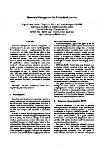
Deferrable server The deferrable server by Strosnider et al. (1995) is bandwidth preserving. This means that when a server is switched out because none of its tasks are ready, it will preserve its budget to handle tasks which may become ready later. A deferrable server can be in one of the states shown in Figure 3.1. A server in the running state is said to be active, and in either ready, waiting or depleted state is said to be inactive. A change from inactive to active or vice-versa is accompanied by the server being switched in or switched out, respectively. replenishment create

Waiting

demand replenishment

demand depletion dispatch

replenishment

Ready

Running

replenishment

preemption replenishment

depletion

Depleted

Figure 3.1: State transition diagram for the deferrable server. A deferrable server s 2 C is created in the waiting state, with its remaining budget equal to its capacity, i.e. (Os , s) = ⇥i . As soon as there is demand for it, it moves to the ready state. When it is dispatched by the scheduler it moves to the running state. A running server s may become inactive for one of three reasons: • It has been preempted by a higher priority server, upon which it preserves its budget and moves to the ready state. • It has remaining budget, but none of its tasks in (s) are ready to run, upon which it preserves its budget and moves to the waiting state. • Its budget has become depleted, upon which it moves to the depleted state. When a depleted server is replenished it moves to the ready state and becomes eligible to run. A waiting server may be woken up by a newly arrived periodic task or a delay event.

28


Idling periodic server When the idling periodic server by Davis and Burns (2005) is replenished and none of the tasks in (s) is ready, then it idles its budget away until either a task arrives or the budget depletes. An idling periodic server follows the state transition diagram in Figure 3.2. It resembles the state transition diagram demand depletion

create

dispatch replenishment

Ready

Running

replenishment

preemption depletion

replenishment

Depleted

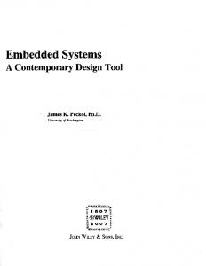
Figure 3.2: State transition diagram for the periodic-idling server. of a deferrable server, however, due to its idling nature the periodic-idling server will never reach the waiting state. The idling property can be regarded as artificial demand for it when there is no proper demand from its tasks. Polling server The polling server by Lehoczky et al. (1987) is not bandwidth preserving. Therefore, when it is replenished and none of the tasks in (s) is ready, or when its workload is exhausted, then its budget is immediately depleted. A polling server can be in one of three states, shown in Figure 3.3. The di↵erence create

dispatch replenishment

Ready

Running

replenishment

preemption depletion or workload exhausted

replenishment

Depleted

Figure 3.3: State transition diagram for the polling server. between a polling and a deferrable server lies in what happens when the workload of

RELTEQ

29

a running server is exhausted. Rather than moving to the waiting state (and thus preserving its budget), the polling server discards any remaining budget and moves to the depleted state. Hierarchical scheduling In two-level hierarchical scheduling one can identify a global scheduler which is responsible for selecting a server component. The server is then free to use any local scheduler to select a task to run. In order to facilitate the reuse of existing server components when integrating them to form larger systems, the platform should support (at least) fixed-priority preemptive scheduling at the local level within servers (since it is a de-facto standard in the industry). To give the system designer the most freedom it should support arbitrary schedulers at the global level. In this chapter we will focus on a fixedpriority scheduler on both local and global level. Timed events The platform needs to support at least the following timed events: task delay, arrival of a periodic task, server replenishment and server depletion, which are generated by the timer handler. Events local to server s, such as the arrival of periodic tasks in (s), should not interfere with other servers, unless they wake a server, i.e. the time required to handle them should be accounted to s, rather than the currently running server. In particular, handling the events local to inactive servers should not interfere with the currently active server and should be deferred until the corresponding server is switched in.

3.3

RELTEQ

Our goal in this chapter is to extend the real-time operating system µC/OS-II with an HSF. To implement the desired extensions in µC/OS-II we needed a general mechanism for di↵erent kinds of timed events, exhibiting low runtime overheads. This mechanism should be expressive enough to easily implement higher level primitives, such as periodic tasks, fixed-priority servers and two-level fixed-priority scheduling.

3.3.1

RELTEQ time model

RELTEQ stores the arrival times of future events relative to each other, by expressing their time relative to their previous event. The arrival time of the head event is relative to the current time2 , as shown in Figure 3.4. 2 Later in this chapter we will use RELTEQ queues as an underlying data structure for di↵erent purposes. We will relax the queue definition: all event times will be expressed relative to their previous event, but the head event will not necessarily be relative to “now”.

30

Processor management now

990

e1

e2

e3

e4

e5

12

4

5

5

10

event time

1002

1006

1011

1016

1026

absolute time

Figure 3.4: Example of the RELTEQ event queue. Unbounded interarrival time between events One of our requirements is for long event interarrival times with respect to time representation. In other words, given d as the largest value that can be represented for a fixed bit-length time representation, we want to be able to express events which are kd time units apart, for some parameter k > 1. For an n-bit time representation, the maximum interval between two consecutive events in the queue is 2n 1 time units3 . Using k events, we can therefore represent event interarrival time of at most k(2n 1). RELTEQ improves this interval even further and allows for an arbitrarily long interval between any two events by inserting “dummy” events, as shown in Figure 3.5. (a)

4

5

n 2 +10

Legend: event

(b)

4

5

2n-1

9

dummy event

Figure 3.5: Example of (a) an overflowing relative event time (b) RELTEQ inserting a dummy event with time 2n 1 to handle the overflow. If t represents the event time of the last event in the queue, then an event ei with a time larger than 2n 1 relative to t can be inserted by first inserting dummy events with time 2n 1 at the end of the queue until the remaining relative time of ei is smaller or equal to 2n 1. In general, dummy events act as placeholders in queues and can be assigned any time in the interval [0, 2n 1].

3.3.2

RELTEQ data structures

A RELTEQ event is specified by the tuple (kind , time, data). The kind field identifies the event kind, e.g. a delay or the arrival of a periodic task. time is the event time. data points to additional data that may be required to handle the event and depends on the event kind. For example, a delay event will point to the task which is to be resumed after the delay event expires. Decrementing an event means decrementing its event time and incrementing an event means incrementing its event time. We will 3 With

n bits we can represent 2n distinct numbers. Since we start at 0, the largest one is 2n

1.

RELTEQ

31

use a dot notation to represent individual fields in the data structures, e.g. ei .time is the event time of event ei . A RELTEQ queue is a list of RELTEQ events. Head(qi ) represents the head event in queue qi .

3.3.3

RELTEQ tick handler

While RELTEQ is not restricted to any specific hardware timer, in this chapter we assume a periodic timer which invokes the tick handler, outlined in Figure 3.6. The tick handler is responsible for managing the system queue, which is a RELTEQ queue keeping track of all the timed events in the system. At every tick of the periodic timer the time of the head event in the queue is decremented. When the time of the head event is 0, then the events with time equal to 0 are popped from the queue and handled. The scheduler is called at the end of the tick handler, but only in case an event was handled. If no event was handled the currently running task is resumed. The behavior of a RELTEQ tick handler is summarized in Figure 3.6. Head(system).time := Head(system).time - 1; if Head(system).time = 0 then repeat HandleEvent(Head(system)); P opEvent(system); until Head(system).time > 0 Schedule(); end if Figure 3.6: Pseudocode for the RELTEQ tick handler. How an event is handled by HandleEvent() depends on its kind. E.g. a delay event will resume the delayed task. In general, the event handler will often use the basic RELTEQ primitives, as described in the following sections. Note that the tick granularity dictates the granularity of any timed events driven by the tick handler: e.g. a server’s budget can be depleted only upon a tick. High resolution one-shot timers (e.g. High Precision Event Timers) provide a fine grained alternative to periodic ticks. In case these are present, RELTEQ can easily take advantage of the fine time granularity by setting the timer to the expiration of the earliest event among the active queues. The tick based approach was chosen due to lack of hardware support for high resolution one-shot timers on our example platform. In case such a one-shot timer is available, our RELTEQ based approach can be easily modified to take advantage of it.

3.3.4

Basic RELTEQ primitives

A new event can be created using the following method:

32


Event NewEvent(Kind k, Time t, Data d ) Creates and returns a new event ei with ei .kind = k, ei .time = t, and ei .data = d. Three operations can be performed on an event queue: a new event can be inserted, the head event can be popped, and an arbitrary event in the queue can be deleted: void InsertEvent(Queue qi , Event ej ) void PopEvent(Queue qi )

Removes the earliest event from qi .

void DeleteEvent(Queue qi , Event ej )

3.3.5

Inserts event ej into queue qi .

Removes event ej from queue qi .

Event queue implementation

The most straightforward RELTEQ queue implementation is probably a doubly linked list: void InsertEvent(Queue qi , Event ej ) When a new event ej with absolute time tj is inserted into the event queue qi , the queue is traversed accumulating the relative times of the events until a later event ek is found, with absolute time tk tj . When such an event is found, then (i) ej is inserted before ek , (ii) its time ej .time is set relative to the previous event, and (iii) the arrival time of ek is set relative to ej (i.e. tk tj ). If no later event was found, then ej is appended at the end of the queue, and its time is set relative to the previous event. void PopEvent(Queue qi ) When an event is popped from a queue it is simply removed from the head of the queue qi . void DeleteEvent(Queue qi , Event ej ) Since all events in a queue are stored relative to each other, the time ej .time of any event ej 2 qi is critical for the integrity of the events later in the queue. Therefore, before an event ej is removed from qi , its event time ej .time is added to the following event in qi . Note that the addition could overflow. In such case, instead of adding ej .time to the following event in qi , the kind of ej is set to a dummy event and the event is not removed. If ej is the last event in qi then it is simply removed, together with any dummy events preceding it. The time complexity of the InsertEvent() operation is then linear in the number of events in the queue, while the complexity of the DeleteEvent() and PopEvent() operations is constant. The linear time complexity of the insert operation may be inconvenient for large event queues. An alternative implementation based on a heap or a balanced binary

Periodic tasks

33

tree may seem more appropriate, as it promises logarithmic time operations. However, as the following theorem states, the relative time representation coupled with the requirement for long event interarrival times (compared to the time representation) make such an implementation impossible. Theorem 3.1. Assume that the maximum value we can represent in the time representation is d and also assume that we store times in a tree using relative values no greater than d. Finally, assume that any two events in the tree are at most kd apart in real time, for some parameter k. Then a logarithmic time retrieval of an event from a tree is not possible. Proof. If there are k events, the largest time span these k events can represent is kd time units, i.e., the time di↵erence between the first and last event can be at most kd units. If we are to obtain this value by summing over a path this path has to be of length k which leads to a linear representation. This argument pertains to any representation that sums contributions over a path. We can illustrate Theorem 3.1 using dummy events: assuming that we start at time 0, the real time of a newly inserted event is at most kd. We would need to insert dummy events until a root path can contain this value. This means we would need to add dummy events until there is a root path of length k. Conversely, if we assume a tree representation, then we would like to obtain kd as a sum of log(k) events. If we assume an even distribution over all events, which is the best case with respect to the number of bits required for the then l time ⇣ representation, ⌘m k k each event time will be equal to log(k) d. This means that log log(k) extra bits are needed. Therefore, in a tree implementation one cannot limit the time representation to a given fixed value, independent of kd (i.e. the tree span). In order to satisfy our initial requirement for long event interarrival time, we chose for a linked-list implementation of RELTEQ queues. In future work we look into relaxing this requirement.

3.4

Periodic tasks

The task concept is an abstraction of a program text. There are roughly three approaches to periodic tasks, depending on the primitives the operating system provides. Figure 3.7 illustrates the possible implementations of periodic tasks, where function fi () represents the body of task ⌧i (i.e. the actual work done during each job of task ⌧i ). In Figure 3.7.a, the periodic behavior is programmed explicitly while in Figure 3.7.b this periodicity is implicit. The first syntax is typical for a system without support for periodicity, like µC/OS-II. It provides two methods for managing time: GetT ime() which returns the current time, and DelayF or(t) which delays the execution of the current task for t time units relative to the time when the method was called. As an important downside, the approach in Figure 3.7.a may give rise to jitter, when the task is preempted between now := GetT ime() and DelayF or().

34


T ask ⌧i : k := 0; while true do now := GetT ime(); DelayF or(Oi + k ⇤ Ti k := k + 1; fi (); end while

Registration: T askM akeP eriodic(⌧i , Oi , Ti ); T ask ⌧i : while true do T askW aitP eriod(); fi (); end while

now);

(a)

(b) Registration: RegisterP eriodic(fi (), Oi , Ti ); (c)

Figure 3.7: Possible implementations of a periodic task. In order to go from Figure 3.7.a to 3.7.c we extract the periodic timer management from the task in two functions: a registration of the task as periodic and a synchronization with the timer system. A straightforward implementation of TaskWaitPeriod() is a suspension on a semaphore. Note that we wait at the beginning of the while loop body (rather than at the end) in case Oi > 0. Going from interface in Figure 3.7.b to 3.7.c is now a simple implementation issue. Note that the task structure described in Figure 3.7.b guarantees that a job will not start before the previous job has completed, and therefore makes sure that two jobs of the same task will not overlap if the first job’s response time exceeds the task’s period.

RELTEQ primitives for periodic tasks In order to provide the periodic task interface in 3.7.b, we need to implement a timer which expires periodically and triggers the task waiting inside the TaskWaitPeriod() call. To support periodic tasks we introduce a new kind of RELTEQ events: a period event. Each period event ei points to a task ⌧i . The expiration of a period event ei indicates the arrival of a periodic task ⌧i upon which (i) the event time of the ei is set to Ti and reinserted into the system queue using InsertEvent(), and (ii) the semaphore blocking ⌧i is raised. To support periodic tasks we have equipped each task with three additional attributes: TaskPeriod , expressed in the number of ticks, TaskPeriodSemaphore, pointing to the semaphore guarding the release of the task, and TaskPeriodEvent, pointing to a RELTEQ period event. For efficiency reasons we have added these directly to the Task Control Block (TCB), which is the µC/OS-II structure storing the state in-

Servers

35

formation about a task. Our extensions could, however, reside in a separate structure pointing back to the original TCB. A task ⌧i is made periodic by calling TaskMakePeriodic(⌧i , Oi , Ti ), which 1. sets the TaskPeriod to Ti , 2. removes the TaskPeriodEvent from the system queue using DeleteEvent(), in case it was already inserted by a previous call to TaskMakePeriodic(), otherwise creates a new period event using NewEvent(period, Ti , ⌧i ) and assigns it to TaskPeriodEvent. 3. sets the event time of the TaskPeriodEvent to Oi if Oi > 0 or Ti if Oi = 0, and inserts it into the system queue.

3.5

Servers

A server s is created using ServerCreate(⇧i , ⇥i , kind), where kind specifies whether the server is idling periodic or deferrable. A task ⌧i is mapped to server s using ServerAddTask(s, ⌧i ). In Section 3.3.3 we have introduced a system queue, which keeps track of pending timed events. For handling periodic tasks assigned to servers we could reuse the system queue. However, this would mean that the tick handler would process the expiration of events local to inactive servers within the budget of the running server. In order to limit the interference from inactive servers we would like to separate the events belonging to di↵erent servers. For this purpose we introduce additional RELTEQ queues for each server. We start this section by introducing additional primitives for manipulating queues, followed by describing how to use these in order to implement fixed-priority servers.

3.5.1

RELTEQ primitives for servers

We introduce the notion of a pool of queues, and define two pools: active queues and inactive queues. They are implemented as lists of RELTEQ queues. Conceptually, at every tick of the periodic timer the heads of all active queues are decremented. The inactive queues are left untouched. To support servers we extend RELTEQ with the following methods: void ActivateQueue(Queue qi ) tive pool.

Moves queue qi from the inactive pool to the ac-

void DeactivateQueue(Queue qi ) inactive pool.

Moves queue qi from the active pool to the

void IncrementQueue(Queue qi ) Increments the head event in queue qi by 1. Time overflows are handled by setting the overflowing event to 2n 1 and inserting a new dummy event at the head of the queue with time equal to the overflow (i.e. 1).

36


void SyncQueueUntilEvent(Queue qi , Queue qj , Event ek ) Synchronizes queue qi with queue qj until event ek 2 qj , by conceptually computing the absolute time of ek , and then popping and handling all the events in qi which have occurred during that time interval.

3.5.2

Limiting interference of inactive servers

To support servers, we add an additional server queue for each server s, denoted by s.sq, to keep track of the events local to the server, i.e. delays and periodic arrival of tasks ⌧j 2 (s). At any time at most one server can be active; all other servers are inactive. The additional server queues make sure that the events local to inactive servers do not interfere with the currently active server. When the active server is switched out (e.g. because a higher priority server is resumed, or the active server gets depleted) then the active server queue is deactivated by calling DeactivateQueue(s.sq). As a result, the queue of the switched out server is “paused”. When a server s is switched in then its server queue is activated by calling ActivateQueue(s.sq). As a result, the queue of the switched in server is “resumed”. The system queue is never deactivated. In this new configuration the hardware timer drives two event queues: 1. the system queue, keeping track of system events, i.e. the replenishment of periodic servers, 2. the server queue of the active server, keeping track of the events local to a particular server, i.e. task delays and the arrival of periodic tasks belonging to the server. To keep track of the time which has passed since the last server switch, we introduce a stopwatch. The stopwatch is basically a counter, which is incremented with every tick. In order to handle time overflows discussed in Section 3.3.1, we represent the stopwatch as a RELTEQ queue and use IncrementQueue(stopwatch) to increment it. During the time when a server is inactive, several other servers may be switched in and out. Therefore, next to keeping track of time since the last server switch, for each server we also need to keep track of how long it was inactive, i.e the time since that particular server was switched out. Rather than storing a separate counter for each server, we multiplex the stopwatches for all servers onto the single stopwatch which we have already introduced, exploiting the RELTEQ approach. We do this by inserting a stopwatch event, denoted by s.se, at the head of the stopwatch queue using InsertEvent(stopwatch, s.se) whenever server s is switched out. The event points to the server and its time is initially set to 0. The behavior of the tick handler with respect to the stopwatch remains unchanged: upon every tick the head event in the stopwatch queue is incremented using IncrementQueue(stopwatch). During runtime the stopwatch queue will contain one stopwatch event for every inactive server (the stopwatch event for the currently active server is removed when the server is switched in). The semantics of the stopwatch queue is defined as follows:

Servers

37

the accumulated time from the head of the queue until (and including) a stopwatch event s.se represents the time the server s was switched out. When a server s is switched in, its server queue is synchronized with the stopwatch using SyncQueuesUntilEvent(s.sq, stopwatch, s.se), which handles all the events in s.sq which might have occurred during the time the server was switched out. It accumulates the time in the stopwatch queue until the stopwatch event s.se and handles all the events in s.sq which have expired during that time. Then s.se is removed from the stopwatch queue. When s is switched out, s.se with time 0 is inserted at the head of the stopwatch queue. Example 3.1. The stopwatch queue is a great example of RELTEQ’s strength. It provides an efficient and concise mechanism for keeping track of the inactive time for all servers. Figure 3.8 demonstrates the behavior of the stopwatch queue for an example system consisting of three servers A, B and C. It illustrates the state of the stopwatch queue at di↵erent moments during execution, before the currently running server is switched out and after the next server is switched in. Legend

A

running server B

0 C

stopwatch event before server switch

0 C

stopwatch event after server switch

C

0 Stopwatch

5 0 A

10

0 B 3 B

15

20 0 B

0 C 0 C

0 C

0 A

4 A

3 C

3 C 2 B

25

0 B

4 A

4 A

0 C 7 C

2 B

2 B 9 C

4 A

4 A 6 A

7 C 0 B

6 A 9 C

Figure 3.8: Example of the stopwatch queue. Initially, when server s is created, a stopwatch event s.se with time 0 is inserted into the stopwatch queue. At time 0 server A is switched in and its stopwatch event is removed. While server A is running, the tick handler increments the head of the stopwatch queue, which happens to be the stopwatch event of server B. At time 3,

38


when server A is switched out and server B is switched in, server B synchronizes its absolute queue with the stopwatch queue until and including B.se, B.se is deleted, and A.se with time 0 is inserted. Note that when B.se is deleted, its time is added to C.se. At time 7 server C is switched in, its absolute queue is synchronized with time 4 + 3 = 7, after which C.se is deleted, and B.se with time 0 is inserted. At time 9, since no server is switched in, no synchronization is taking place and no stopwatch event is deleted. Only stopwatch event C.se with time 0 is inserted, since server C is switched out. At time 16, when server B is switched in and its stopwatch event B.se is deleted, the time of B.se is added to C.se. Deferrable server When the workload of a deferrable server s is exhausted, i.e. there are no ready tasks in (s), then the server is switched out and its server queue s.sq is deactivated. Consequently, any periodic task which could wake up the server to consume any remaining budget cannot be noticed. One could alleviate this problem by keeping its server queue active when s is switched out. This, however, would make the tick handler overhead linear in the number of deferrable servers, since a tick handler decrements the head events in all active queues (see Section 3.5.6). Instead, in order to limit the interference of inactive deferrable servers, when a deferrable server s is switched out and it has no workload pending (i.e. no tasks in (s) are ready), we deactivate s.sq, change its state to waiting, and insert a wakeup event, denoted as s.we, into the system queue. The wakeup event has its data pointing to s and time equal to the arrival of the first event in s.sq. When the wakeup event expires, the state of s is set to the ready state. This way handling the events inside s.sq is deferred until s is switched in. Idling periodic server An idling periodic server is a special kind of a deferrable server containing an idle task (with lowest priority). The idle task is switched in if no higher priority task is ready, e↵ectively idling away the remaining capacity. In order to save memory needed for storing the task control block and the stack of the idle task, one idle task is shared between all idling periodic servers in the system.

3.5.3

Virtual timers

When the server budget is depleted an event must be triggered to guarantee that a server does not exceed its budget. In the next section we present a general approach for handling server depletion. It relies on the notion of virtual timers, which are events relative to server’s budget consumption. These compliment the global timers, which operate in the absolute time domain, used for triggering events such as server replenishment or the arrival of periodic tasks.

Servers

39

We can implement virtual timers by adding a virtual server queue for each server, denoted by s.vq. Similarly to the server queues introduced earlier, when a server is switched in, its virtual server queue is activated. The di↵erence is that the virtual server queue is not synchronized with the stopwatch queue, since during the inactive period a server does not consume any of its budget. When a server is switched out, its virtual server queue is deactivated. The relative time representation by RELTEQ allows for a more efficient virtual queue activation than an absolute time representation does. An absolute time representation (e.g. in (Behnam et al., 2008; Inam et al., 2011)) requires to recompute the expiration time for all the events in a virtual server queue upon switching in the corresponding server, which is linear in the number of events. In our RELTEQ-based virtual queues the events are stored relative to each other and their expiration times do not need to be recomputed upon queue activation. Note that it will never be necessary to handle an expired virtual event upon queue activation, since such an event would have been already handled before the corresponding server was switched out. Therefore, our HSF design exhibits a constant time activation of a virtual server queue.

3.5.4

Server replenishment and depletion

We introduce two additional RELTEQ event kinds to support servers: server replenishment and server depletion. When a server s is created, a replenishment event ej is inserted into the system queue, with ej .data pointing to s and ej .time equal to the server’s replenishment period ⇧i . When ej expires, ej .time is updated to ⇧i and it is inserted into the system queue. Upon replenishment, the server’s depletion event ej is inserted into its virtual server queue, with ej .data pointing to s and ej .time equal to the server’s capacity ⇥i . If the server was not depleted yet, then the old depletion event is removed from the virtual server queue using DeleteEvent(s.vq, ej ).

3.5.5

Switching servers

The methods for switching servers in and out are summarized in Figures 3.9 and 3.10. SyncQueuesUntilEvent(s.sq, stopwatch, s.se); ActivateQueue(s.sq); ActivateQueue(s.vq); if s.we 6= ; then DeleteEvent(system, s.we); s.we = ;; end if Figure 3.9: Pseudocode for ServerSwitchIn(s).

40


DeleteEvent(stopwatch, s.se); s.se = NewEvent(stopwatch, 0, s); InsertEvent(stopwatch, s.se); DeactivateQueue(s.sq); DeactivateQueue(s.vq); if s.readyT asks = ; then s.we = NewEvent(wakeup, Head(s.sq).time, s); InsertEvent(system, s.we); end if Figure 3.10: Pseudocode for ServerSwitchOut(s).

3.5.6

RELTEQ tick handler with support for servers

An example of the RELTEQ queues managed by the tick handler in the proposed RELTEQ extension with servers is summarized in Figure 3.11. Conceptually, every system queue

56

4

5

2n-1

stopwatch queue

7

27

2n-1

3

active server queue

17

21

27

5

101

23

2n-1

34

37

4

active virtual server queue

inactive server queues & virtual server queus

Legend:

10

3

event

head of an active queue which is decrementd

dummy event

head of an active queue which is incremented

Figure 3.11: Example of the RELTEQ queues managed by the tick handler. tick the stopwatch queue is incremented and the heads of the system queue, the active server queue and the active virtual server queue are decremented. If the head of any queue becomes 0, then their head event is popped and handled until the queue is

Servers

41

exhausted or the head event has time larger than 0. Actually, rather than decrementing the head of each active queue and checking whether it is 0, a CurrentTime counter is incremented and compared to the EarliestTime, which is set whenever the head of an active queue changes. If they are equal, then (i) the CurrentTime is subtracted from the heads of all the active queues, (ii) any head event with time 0 is popped and handled, (iii) CurrentTime is set to 0, and (iv) EarliestTime is set to the earliest time among the heads of all active queues4 . The behavior of a RELTEQ tick handler supporting servers is summarized in Figure 3.12. IncrementQueue(stopwatch); CurrentT ime := CurrentT ime + 1; if EarliestT ime = CurrentT ime then for all q 2 activequeues do Head(q).time := Head(q).time CurrentT ime; while Head(q).time = 0 do HandleEvent(Head(q)); P opEvent(q); end while end for CurrentT ime := 0; EarliestT ime := Earliest(activequeues); Schedule(); end if Figure 3.12: Pseudocode for the RELTEQ tick handler supporting hierarchical scheduling. Note that at any moment in time there are at most four active queues, as shown in Figure 3.11. Also, the tick handler is executed with disabled interrupts, guaranteeing mutually exclusive access to the queue data structures.

3.5.7

Summary

We have described a generic framework for supporting servers, which is tick based (Section 3.3.3) and limits the interference of inactive servers on system level (Section 3.5.2). The interference of inactive servers which are either ready or depleted was limited by means of a combination of inactive server queues and a stopwatch queue. Deactivating server queues of waiting servers was made possible by inserting a wakeup event into the system queue, in order to wake up the server upon the arrival of a periodic task while the server is switched out. A large part of our design concerns manipulating events in di↵erent event queues. Table 3.1 summarizes which events are stored in which queues. Note that each queue 4 Note

that the time of any event will never become negative.

42


can contain dummy events to prolong the event inter-arrival times. Queue System queue Stopwatch queue Server queue Server virtual queue

Events Server replenishment, server wakeup Stopwatch event Periodic task arrival, task delay Server depletion

Table 3.1: Mapping between events and queues.

3.6

Hierarchical scheduling

Rajkumar et al. (1998) identified four ingredients necessary for guaranteeing resource provisions: admission, monitoring, scheduling and enforcement. In this section we describe how our implementation of HSF addresses each of them.

3.6.1

Admission

We allow admission of new components only during the integration, not during runtime. The admission testing requires analysis for hierarchical systems, which is outside the scope of this chapter.

3.6.2

Monitoring

There are two reasons for monitoring the budget consumption of servers: (i) handle the server depletion and (ii) allow the assigned tasks to track and adapt to the available budget. In order to notice the moment when a server becomes depleted we have introduced a virtual depletion event for every server, which is inserted into its virtual server queue. When the depletion event expires, then (i) the server’s capacity is set to 0, (ii) its state is set to depleted, and (iii) the scheduler is called. We would like to allow tasks ⌧j 2 (s) to track the remaining server budget s . Upon such a request, we could sum up the event times of the depletion event of server s and all the previous events in the virtual server queue. However, this approach would incur an overhead linear in the number of events in the virtual server queue upon every request for the remaining budget. We therefore equipped each server with a budget counter. Upon every tick the budget counter of the currently active server is decremented by one. The depletion event will make sure that a depleted server is switched out before the counter becomes negative. We also added the ServerBudget() method, which can be called by any task. Ticks ServerBudget(Server s) Returns the current value of i , which represents the lower bound on the processor time that server s will receive within the remainder of its current period.

Hierarchical scheduling

3.6.3

43

Scheduling

The µC/OS-II the scheduler does two things: (i) select the highest priority ready task, and (ii) in case it is di↵erent from the currently running one, do a context switch. Our hierarchical scheduler replaces the original OS SchedNew() method, which is used by the µC/OS-II scheduler to select the highest priority ready task. It first uses the global scheduler HighestReadyServer() to select the highest priority ready server, and then the server’s local scheduler HighestReadyTask(), which selects the highest priority ready task belonging to that server. This approach allows to implement di↵erent global and local schedulers (such as fixed-priority or EDF), and also di↵erent schedulers in each server. Our fixed-priority global scheduler is shown in Figure 3.13. highestServer := HighestReadyServer(); if highestServer 6= currentServer then if currentServer 6= ; then ServerSwitchOut(currentServer); end if if highestServer 6= ; then ServerSwitchIn(highestServer); end if currentServer := highestServer; end if if currentServer 6= ; then return currentServer.HighestReadyT ask(); else return idleT ask; end if Figure 3.13: Pseudocode for the hierarchical scheduler. The currentServer is a global variable referring to the currently active server. Initially currentServer = ;. The scheduler first determines the highest priority ready server. Then, if the server is di↵erent from the currently active server, a server switch is performed, composed of 3 steps: 1. If there is a currently active server, then it is switched out, using ServerSwitchOut() described in Section 3.5.5. 2. If there is a ready server, then it is switched in, using ServerSwitchIn() described in Section 3.5.5. 3. The currentServer is updated. Finally the highest priority task in the currently active server is selected, using the current server’s local scheduler HighestReadyTask(). If no server is active, then the idle task is returned.

44

3.6.4


Enforcement

When a server becomes depleted during the execution of one of its tasks (i.e. if a depletion event expires), the task will be preempted and the server will be switched out. This is possible, since we assume preemptive and independent tasks.

3.7

Evalulation

Figure 3.14 shows a trace of an example application consisting of two servers, each serving one task. We ran the setup within the OpenRISC simulator (OpenCores, 2010), with 1 tick set to 1ms5 . The task execution is shown on top, with the server capacities illustrated underneath. The application was traced and visualized using the Grasp toolset (see Chapter 6).

Task1

Task2

uC/OS-II Idle

10 Deferrable Server

5 0 10

Periodic Server

5 0

0

50

100

Figure 3.14: Example trace of an application with one deferrable and one periodic idling server. In this particular example Task1 is assigned to the Deferrable Server, and Task2 is assigned to the Periodic Server. Both tasks have a period of 30ms and execution 5 The complete simulation setup and the source code of our HSF realization are available at http://www.win.tue.nl/~mholende/ucos/.

Evalulation

45

time of 5ms. Task1 has an o↵set of 5ms. Both servers have a replenishment period of 25ms and capacity of 10ms. The figure demonstrates, how the idling periodic server idles away its capacity when there is no workload pending (time interval 10-15ms), while the deferrable server preserves its capacity until Task1 arrives (time interval 25-35ms). The figure also illustrates how the handling of period events (indicated by the arrows) of Task2 is postponed until the Periodic Server is switched in (at time 50ms). In the remainder of this section we evaluate the modularity, memory footprint and performance of the HSF extension for RELTEQ. We chose a linked-list as the data structure underlying our RELTEQ queues and implemented the proposed design within µC/OS-II.

3.7.1

Modularity and memory footprint

The design of RELTEQ and the HSF extension is modular, allowing to enable or disable the support for HSF and di↵erent server types during compilation with a single compiler directive for each extension. The complete RELTEQ implementation including the HSF extension is 1610 lines of code (excluding comments and blank lines), compared to 8330 lines of the original µC/OS-II. 105 lines of code were inserted into the original µC/OS-II code, out of which 60 were conditional compilation directives allowing to easily enable and disable our extensions. No original code was deleted or modified. Note that the RELTEQ+HSF code can replace the existing timing mechanisms in µC/OS-II, and that it provides a framework for easy implementation of other scheduler and servers types. The 105 lines of code represent the e↵ort required to port RELTEQ+HSF to another operating system. Such porting requires (i) redirecting the tick handler to the RELTEQ handler, (ii) redirecting the method responsible for selecting the highest priority task to the HSF scheduler, and (iii) identifying when tasks become ready or blocked. The memory footprint of RELTEQ+HSF is summarized in Table 3.2. It lists the additional memory required by and application consisting of 6 servers with 6 tasks each using µC/OS-II+RELTEQ+HSF, compared to the memory requirements of an application consisting of 36 tasks (with a stack of 128B each) using the original µC/OS-II.

Code Data

µC/OS-II 32KB 47KB

RELTEQ+HSF 8KB 5KB

Table 3.2: Memory overhead of RELTEQ+HSF.

46


3.7.2

Performance analysis

In this section we evaluate the system overheads of our extensions, in particular the overheads of the scheduler and the tick handler. We express the overhead in terms of the maximum number of events inside the queues which need to be handled in a single invocation of the scheduler or the tick handler, times the maximum overhead for handling a single event. Handling a single event Handling di↵erent events will result in di↵erent overheads. • When a dummy event expires, it is simply removed from the head of the queue. Hence, handling it requires O(1) time. • When a task period event expires, an event representing the next periodic arrival is inserted into the corresponding server queue. In this section we assume a linked-list implementation, and consequently insertion is linear in the number of events in a queue. Note that we could delay inserting the next period event until the task completes, as at most one job of a task may be running at a time. This would reduce the handling of a periodic arrival to constant time, albeit at the additional cost of keeping track for each task of the time since its arrival, which would be taken into account when inserting the next period event. However, if we would like to monitor whether tasks complete before their deadline, then we will need to insert a deadline event into s.sq anyway. Hence the time for handling an event inside of a server queue is linear in the number of events in a server queue. Since there are at most two events per task in a server queue (period and deadline events), handling a period event is linear in the maximum number of tasks assigned to a server, i.e. O(m(s)). • When a task deadline event expires, it is simply removed from the head of the queue an the system is notified that a deadline was missed. Hence, handling it requires O(1) time. • When a server replenishment event expires, an event representing the next replenishment is inserted into the system queue6 . Since there are at most two events in the system queue per server (replenishment and wakeup event), handling a replenishment event is linear in the number of servers, i.e O(|⌃|). • When a server depletion event expires, it is simply removed from the queue. Hence, handling it requires O(1) time. 6 Inserting the next replenishment event could be deferred until the server is depleted, at a similar cost and benefit to deferring the insertion of the task period event.

Evalulation

47

Scheduler Our HSF supports di↵erent global and local schedulers, by means of the methods HighestReadyServer() and HighestReadyTask(). For the sake of a fair comparison with the µC/OS-II which implements a fixed-priority scheduler, we also assume fixed-priority global and local schedulers in this section. For both global and local scheduling we can reuse the bitmap-based approach implemented by µC/OS-II, which has a constant time overhead for selecting the highest priority ready task as well as indicating whether a task is ready or not (Labrosse, 2002). Consequently, in our HSF we can select the highest priority server and task within a server in constant time. Once a highest priority server s is selected, the overhead of switching in the server depends on the number of events inside the stopwatch queue and s.sq (which needs to be synchronized with the stopwatch), and the overhead of selecting the highest priority task. The stopwatch queue contains one stopwatch event for each inactive server. The length of the stopwatch queue is therefore bounded by |⌃| + ds , where |⌃| is the k j ts (s) number of servers, and ds = maxs2⌃ 2n 1 is the maximum number of dummy events inside the stopwatch queue. ts (s) is the longest time interval that a server can be switched out, and 2n 1 is the largest relative time which can be represented with n bits. The only local events are a task delay and the arrival of a periodic task. Also, each task can wait for at most one timed event at a time. The number of events inside the server queue is therefore bounded by m(s) + dlj(s), where m(s) is the maximum k number of tasks assigned to server s, and dl (s) =

tl (s) 2n 1

is the maximum number

of dummy events local to the server queue s.sq. tl (s) is the longest time interval between any two events inside of s.sq (e.g. the longest task period or the longest task delay). The complexity of the scheduler is therefore O(|⌃| + ds + m(s) + dl (s)). Note that the maximum numbers of dummy events ds and dl (s) can be determined at design time. Tick handler

The tick handler synchronizes all active queues with the current time, and (in case an event was handled) calls the scheduler. The active queues are comprised of the system queue and two queues for the server s which is active at the time the tick handler is invoked (its server queue s.sq and virtual server queue s.vq). The system queue contains only replenishment j and k wakeup events. Its size is tg therefore proportional to |⌃| + dg , where dg = 2n 1 is the maximum number of dummy events inside the global system queue. tg is the longest time interval between any two events inside the global system queue (i.e. the longest server period). The size of s.sq is linear in the number of tasks assigned to the server. Similarly, since s.vq contains one depletion event and at most one virtual timer for each task,

48


its size is linear in the number of tasks assigned to the server. Therefore, when server s is active at the time the tick handler is invoked, the tick handler will need to handle tt (s) = |⌃| + dg + m(s) + dl (s) events. The complexity of the tick handler is therefore O(maxs2⌃ m(s)tt (s)). Note that the tick handler overhead depends only on tasks belonging to the server s which is active at the time of the tick. It does not depend on tasks belonging to other servers. The tick handler keeps track of the remaining budget of servers by decrementing the counter corresponding to the server which is active at the moment of the tick. Consequently, the server that is active at the moment of the tick is charged the entire previous tick. Therefore, any scheduler invocations during a tick interval (including those triggered by the tick handler itself) are executed within the budget of the server which is active at the moment of the following tick. Experimental results In Section 3.5.2 we introduced wakeup events in order to limit the interference due to inactive servers. In order to validate this approach we have also implemented a variant of the HSF scheduler which avoids using wakeup events and instead, whenever a deferrable server s is switched out, it keeps the server queue s.sq active. Consequently, the scheduler does not need to synchronize the server queue when switching in a server. However, this overhead is shifted to the tick handler, which needs to handle the expired events in all the server queues from inactive deferrable servers. In the following discussion we refer to this approach as without limited interference, as opposed to with limited interference based on wakeup events. Figures 3.15, 3.16 and 3.17 compare the two variants. We have varied the number of deferrable servers and the number of tasks assigned to each server (all servers had the same number of tasks). The server replenishment periods and the task periods were all set to the same value (100ms), to exhibit the maximum overhead by having all tasks arrive at the same time. Each task had a execution time of 1ms and each server had a capacity of 7ms. We have run the setup within the cycle-accurate hardware simulator for the OpenRISC 1000 architecture (OpenCores, 2010). We have set the processor clock to 345MHz and the tick to 1KHz, which is inline with the platform used by our industrial partner. Each experiment was run for an integral number of task periods. Figure 3.15 shows the maximum measured overheads of the scheduler and the tick handler, while Figure 3.16 shows the total overhead of the scheduler and the tick handler in terms of processor utilization. The figures demonstrate that wakeup events reduce the tick overhead, at the cost of increasing the scheduler overhead, by e↵ectively shifting the overhead of handling server’s local events from the tick handler to the scheduler. Since the scheduler overhead is accounted to the server which is switched in, as the number of servers and tasks per server increase, so does the advantage of the limited interference approach. Figure 3.17.a combines Figures 3.16.a and 3.16.b and demonstrates that the additional overhead due to the wakeup events in the limited interference approach is negligible. Figure 3.17.b compares the system overheads of our HSF extension to the standard

Evalulation

49

Number of instructions (x1000)

With limited interference Without limited interference

7 6 5 4 3 2 1 01

6 5 2

4 3 Numbe

3 4 r of serv ers

5

2 6 1

ber

of

ks

tas

per

v ser

er

m

Nu

(a)



10 9 8 7 6 5 4 3 2 1 01

6 5 2

4 3 Numbe

3 4 r of serv

5

ers

2 6 1

v ser

er

sk

f ta

o ber

er sp

m

Nu

(b) Figure 3.15: (a) maximum overhead of the (local + global) scheduler, (b) maximum overhead of the tick handler.

µC/OS-II implementation. As the standard µC/OS-II does not implement hierarchical scheduling, we have implemented a flat system containing the same number of tasks with the same parameters as in Figure 3.17.a. The results demonstrate the temporal isolation and efficiency of our HSF implementation. While the standard

50


µC/OS-II scans through all tasks on each tick to see if any task delay has expired, in the HSF extension the tick handler needs to consider only head event in the server queue of the currently running server. Figures 3.18 and 3.19 compare the best-case and worst-case measured overheads of the scheduler and tick handler between µC/OS-II with our extensions, compared to the standard µC/OS-II, for which we have implemented a flat system containing the same number of tasks with the same parameters as for the µC/OS-II+HSF case. Figures 3.18 and 3.19 show that both scheduler and tick handler su↵er larger execution time jitter under µC/OS-II+HSF, than the standard µC/OS-II. In the best case the µC/OS-II+HSF tick handler needs to decrement only the head of the system queue, while in µC/OS-II the tick hander traverses all the tasks in the system and for each one it checks whether its timer has expired. In a system with small utilization of individual tasks and servers (as was the case in our experiments), most local events will arrive while the server is switched out. Since handling local events is deferred until the server is switched in and its server queue synchronized with the stopwatch queue, it explains why the worst-case tick handler overhead is increasing with the number of servers and the worst-case scheduler overhead is increasing with the number of tasks per server.

3.8

Discussion

We have presented an efficient, modular and extensible design for enhancing a realtime operating system with a two-level HSF. It relies on Relative Timed Event Queues (RELTEQ), a general timer management system targeting embedded systems. Our design supports various server types (including polling, idling periodic, and deferrable servers), and global and virtual timers. It supports fixed-priority and EDF schedulers on both local and global level. It provides temporal isolation between components and limits the interference of inactive servers on the active server, by means of wakeup events and a combination of inactive server queues with a stopwatch. Enforcement is provided by means of depletion events, which preempt any running task in the depleted server. This is possible since we assume independent tasks. Monitoring is provided by means of an interface which returns a lower bound on the processor time that a server will receive during the following time interval equal to its period. We have evaluated a fixed-priority based implementation of our RELTEQ and HSF within the µC/OS-II real-time operating system used in the automotive domain. The results demonstrate that our approach exhibits low performance overhead and limits the necessary modifications of the underlying operating system. We have assumed a linked-list implementation of our RELTEQ queues, and indicated the challenges of a tree-based implementation due to the relative time representation. In the future we want to investigate in more detail other advanced data structures for implementing RELTEQ queues.

Discussion

51

Overhead (% processor time)


1 0.9 0.8 0.7 0.6 0.5 0.4 0.3 0.2 0.1 01

6 5 2

4 3 Numbe

3 4 r of serv ers

5

2 6 1

f ro

ks

tas

per

v ser

er

e

mb

Nu

(a)



1.4 1.2 1 0.8 0.6 0.4 0.2 01

6 5

2

4 3 Numbe

3 4 r of serv ers

5

2 6 1

ber

of

ks

tas

v ser per

er

m

Nu

(b) Figure 3.16: (a) total overhead of the scheduler, (b) total overhead of the tick handler.

52




1.8 1.6 1.4 1.2 1 0.8 0.6 0.4 0.2 01

6 5 2

4 3

3 Numbe

4 r of serv ers

5

2 6 1

ber

of

ks

tas

per

ver

ser

m

Nu

(a)


µC/OS-II + HSF µC/OS-II

7 6 5 4 3 2 1 01

6 5 2

4 3 Numbe

3 4 r of serv ers

5

2 6 1

er sp

ver

ser

sk f ta

o ber

m

Nu

(b) Figure 3.17: Total overhead of the tick handler and the scheduler.

Discussion

53


Max scheduler overhead Min scheduler overhead

7 6 5 4 3 2 1 01

6 5 2

4 3 Numbe

3 4 r of serv ers

5

2 6 1

f ro

ks

tas

per

v ser

er

e

mb

Nu

(a)


Max scheduler overhead Min scheduler overhead

0.09 0.08 0.07 0.06 0.05 0.04 0.03 0.02 0.01 01

6 5

2

4 3 Numbe

3 4 r of serv ers

5

2 6 1

ber

of

ks

tas

v ser per

er

m

Nu

(b) Figure 3.18: (a) scheduler overhead in µC/OS-II+HSF, (b) scheduler overhead in µC/OS-II.

54



Max tick handler overhead Min tick handler overhead

7 6 5 4 3 2 1 01

6 5 2

4 3

3 Numbe

4 r of serv ers

5

2 6 1

f ro

ks tas

per

ver

ser

e

mb

Nu

(a)


Max tick handler overhead Min tick handler overhead

3 2.5 2 1.5 1 6

0.5 01

5 2

4 3

3 Numbe

4 r of serv ers

5

2 6 1

ber

of

ks

tas

r rve

se per

m

Nu

(b) Figure 3.19: (a) tick handler overhead in µC/OS-II+HSF, (b) tick handler overhead in µC/OS-II.

Chapter 4

Memory management In this chapter, we focus on memory management in resource constrained embedded systems, where several applications execute on a single processor. We present a set of general techniques targeted at streaming, or data driven, systems, and use example multimedia processing applications for illustration and motivation.

Problem statement In this chapter we address three Quality of Service (QoS) related problems in resource constrained multimedia systems: • Multimedia applications are known to be data intensive. Many of these applications, especially in the consumer electronics domain, are implemented on resource-constrained embedded systems where the memory space is scarce (Yim et al., 2004; Menichelli and Olivieri, 2009; Ahn et al., 2009). Reducing the memory requirements of these applications is therefore crucial. • Hentschel et al. (2003) present the theory and practice of video QoS for Consumer Terminals. They describe a pipelined multimedia processing application, where a multiplexed audio and video input stream is demultiplexed into two bu↵ers and processed independently by two processing subchains, as shown in Figure 4.1. They observe that fluctuation in the processing time for decoding di↵erent video frames may fill up the bu↵ers along the video processing subchain, leading to the blocking of the demultiplexer and consequently the dropping of audio frames, manifested by sound artifacts. The problem arises due to temporal dependencies between component subchains sharing a common predecessor. • The third problem we address in this chapter is bounding the mode change latency in scalable multimedia applications, distinguishing between the application latency and the system latency. From the application perspective, a mode change may interfere with the processing of a video stream. A large 55

56

Memory management Application

DVD player

audio decoder

audio renderer

bv

video decoder

sharpness enhancer

TV

demultiplexer

reader

Digital camera

Legend:

ba

scaler

internal data flow

mixer

external data flow

software component

hardware component

buffer component

Figure 4.1: Block diagram of the system implementation on a multimedia processor presented in Hentschel et al. (2003). The demultiplexer component writes to two output bu↵ers: the audio output bu↵er ba and the video output bu↵er bv . mode change latency will delay the rendering of frames and lead to artifacts in the output video. From the system perspective, during a mode change, resources can be allocated to applications in the new mode only after they have been released by the applications in the old mode. Therefore the mode change latency will impact when the resources can be reallocated between applications and when these applications can resume operating in the new mode.

Contributions The contribution of this chapter is three fold. • Section 4.3 shows how a shared memory pool can reduce the total memory requirements of an application comprised of a data-driven chain of components communicating via bounded bu↵ers, with a time-driven head and tail, and a bounded end-to-end latency. The necessary bu↵er capacities and component priorities along the component chain are derived. Subsequently it is shown how a shared memory pool can reduce the total memory requirements of the whole application. The general technique targeted at memory-constrained streaming systems is demonstrated with a video encoding example, showing memory savings of about 19%. The impact of a shared memory pool is also evaluated in the context of scalable applications. • In Section 4.4, it is shown how additional access to the bu↵er, in particular the support for dropping selected frames, allows to guarantee the QoS of the application during overload conditions, preventing congestion in one bu↵er to propagate across the whole application. In particular, we present an approach which prevents the demultiplexer in Figure 4.1 from blocking.

Related work

57

• In Section 4.5, two approaches are presented for reducing the mode change latency bound in scalable multimedia processing applications, which can adapt their memory requirements during runtime according to a set of predefined modes. The first approach relies on fixed-priority scheduling with deferred preemption to shorten the time between a mode change request and the time when the mode change starts. The second approach applies in-bu↵er scaling to reduce the duration of the mode change itself.

Publications In (Holenderski et al., 2011b,c) we describe how to reduce the memory requirements in a multimedia streaming application. In (Holenderski et al., 2009a,b, 2010b) we describe how to reduce the mode change latency in scalable applications.

4.1 4.1.1

Related work Memory management in embedded systems

In Geelen (2005), systems are investigated which can change their functionality during runtime, by varying their sets of components. Their notion of dynamic functionality is similar to the concept of scalability discussed in Section 4.1.4, where the total memory requirements are determined by the current application mode. They propose a method for dynamic loading of memory in real-time systems. They present a case study of a DVD player platform, with a memory management unit present but disabled, which uses static memory partitioning for memory management. They propose a method with the memory management unit enabled for dividing the memory requirements into static overlays, created during the initialization phase. An overlay groups together the memory requirements of several components belonging to a particular mode (e.g. dvd playback or tv recording). They also show how to manage the loading and storing of overlays between RAM and hard disk by directly controlling the entries in a TLB, and implement their approach in a particular DVD player product. They assume soft deadlines on the mode changes, aiming at providing QoS in terms of “smooth” transitions. In this thesis we present an approach for dynamic reallocation of memory between components during runtime, on a platform without a memory management unit. We organize the memory requirements of components into memory budgets, which components can request, resize and discard during runtime. We show how the components can resize their budgets during a mode change, before the memory can be reallocated to other components. Our approach is well suited for platforms with explicitly managed local memory, such as scratch-pad memory. A scratch-pad provides low latency data storage, similar to on-chip caches, but under explicit software control. The simple design and predictable nature of scratchpad memories has seen them incorporated into a number of embedded and real-time system processors Brash (2002). McIlroy et al. (2008) present a dynamic run-time heap management algorithm for scratch-pad memory.

58

Memory management

Their approach is based on a combination of fixed-sized macro blocks, which are later subdivided into variable sized allocations. In this thesis, we assume the memory is managed in terms of fixed sized blocks (e.g. single bytes or multiple of bytes), allowing to easily reallocate memory between components. We use the notion of memory reservations, which are defined as containers for memory allocations, allowing components to request memory and guarantee granted requests during runtime, avoiding static memory allocation in the absence of paging support. Memory reservations are granted to components only if there is enough space in the common memory pool, and memory allocations are granted only if there is enough space within the corresponding reservation.

4.1.2

Memory reservations

Nakajima (1998) apply memory reservations in the context of continuous media processing applications. They aim at reducing the number of memory pages wired in the physical memory at a time, by wiring only those pages which are used by threads currently processing the media data in the physical memory. Unlike the traditional approaches which avoid page faults by wiring all code, data and stack pages, they introduce an interface to be used by the real-time applications to request reservations for memory pages. During runtime, upon a page fault, the system will load the missing page only if it does not exceed the application’s reservation. Thus the number of wired pages is limited. Eswaran and Rajkumar (2005) implement memory reservations in Linux to limit the time penalty of page faults within the reservation, by isolating the memory management of di↵erent applications from each other. They distinguish between hard and firm reservations, which specify the maximum and minimum number of pages used by the application, respectively. Their reservation model is hierarchical, allowing child reservations to request space from a parent reservation. Their energy-aware extension of memory reservations allows to maximize the power savings, while minimizing the performance penalty, in systems where di↵erent hardware components can operate in di↵erent power levels and corresponding performance levels. They also provide an algorithm which calculates the optimal reservation sizes for the task set such that the sum of the task execution times is minimized. In this thesis we use (hard) memory reservations as containers for memory allocations, allowing components to request memory and guarantee granted requests during runtime, avoiding static memory allocation in the absence of paging support. Memory reservations are granted to components only if there is enough space in the common memory pool, and memory allocations are granted only if there is enough space within the corresponding reservation.

4.1.3

Reducing memory requirements

Optimizing memory usage in resource-constrained devices is becoming increasingly important with the increasing number of mobile and multimedia applications. Yim et al. (2004) present an approach for reducing the internal memory fragmentation in

Related work

59

flash memory for mobile devices. Ahn et al. (2009) consider memory-constrained portable media players and propose a memory allocation scheme for multimedia stream bu↵ers, which allows reducing the number of page faults in heap and thus helps multimedia players perform with a consistent quality. Kim et al. (2010) propose a region reuse technique, based on storing objects in upper local regions to the disk and reusing the reclaimed space for new object allocations, and hence reducing heap memory usage in mobile consumer devices with very limited memory. In contrast to (Yim et al., 2004; Ahn et al., 2009; Kim et al., 2010), which try to manage the memory requirements dictated by the applications, in this thesis we focus on actually reducing the memory requirements. We↵ers-Albu (2008) explores how the assignment of task priorities and bu↵er capacities impact the behavior of multimedia streaming applications comprised of a task chain. The author shows that a task chain with a time-driven tail exhibiting varying task execution times (where processing a window of M consecutive frames is bounded by M T ) will meet its real-time constraints if the last bu↵er has capacity for M frames. They also show that a task chain with a time-driven head and tail, and M = 2, will meet its real-time constraints if all bu↵ers have capacity 1. In this thesis we derive the bu↵er capacities for a chain consisting of a time-driven head and tail and an arbitrary M . Goddard 0 studies the real-time properties of PGM dataflow graphs, which closely resemble our media processing graphs. Given a periodic input and the dataflow attributes of the graph, exact node execution rates are determined for all nodes. The periodic tasks corresponding to each node are then scheduled using a preemptive Earliest Deadline First algorithm. For this implementation of the graph, the author shows how to bound the response time of the graph and the bu↵er requirements. However, it is limited to task sets with deadlines equal to the period, i.e. without self-interference. This approach provided valuable insights, but no rigorous support for analyzing and steering system behavior and associated resource needs has resulted. Though we consider variations in execution time, we do not consider overload problems resulting from the inability to process the input in time. Approaches aiming at that situation can be used to prevent this from happening (Isovic and Fohler, 2004; W¨ ust et al., 2005), or to deal with it when it happens, through scaling or skipping the media content (Lan et al., 2001; W¨ ust et al., 2005; Jarnikov et al., 2004). In (Holenderski et al., 2010b) we investigated scalable applications, which can operate in one of several predefined modes, where each mode specifies the resource requirements in terms of M for all the bu↵ers belonging to the application. We showed how to use in-bu↵er scaling to reduce the memory requirements of each bu↵er. Upon a mode change request for a mode with a smaller M and smaller memory requirements, we would drop the least significant frames from the chain and/or reduce the number of blocks for certain frames, and show how this could reduce the mode change latency. In this thesis we concentrate on how a shared memory pool will a↵ect the memory requirements of a scalable application in di↵erent modes.

60

Memory management

4.1.4

Scalable applications and mode changes

Multimedia processing systems are characterized by few but resource intensive tasks, communicating in a pipeline fashion. The tasks require a processor for processing the video frames (e.g. encoding, decoding, content analysis), and memory for storing intermediate results between the pipeline stages. The pipeline nature of task dependencies poses restrictions on the lifetime of the intermediate results in the memory. The large gap between the worst-case and average-case resource requirements of the tasks is compensated by bu↵ering and their ability to operate in one of several predefined modes, allowing to trade o↵ their processor requirements for quality (W¨ ust et al., 2005), or network bandwidth requirements for quality (Jarnikov et al., 2004). In this thesis we investigate trading memory requirements for quality. We assume there is no memory management unit available. (Real and Crespo, 2004) present a comprehensive survey of mode change protocols for FPPS on a single processor, where modes express the application’s processor requirements, and propose several new protocols along with their corresponding schedulability analysis and configuration methods. They consider a standard fixed priority sporadic task model, with task ⌧i specified by its priority i (lower i meaning higher priority), minimum interarrival period Ti , worst-case execution time Ci , and deadline Di , with 0 < Ci  Di  Ti . They classify existing mode change protocols according to three dimensions: 1. Ability to abort old-mode tasks upon a mode change request: (a) All old-mode tasks are immediately aborted. (b) All old-mode tasks are allowed to complete normally. (c) Some tasks are aborted. 2. Activation pattern of unchanged tasks during the transition: (a) Protocols with periodicity, where unchanged tasks are executed independently from the mode change in progress. (b) Protocols without periodicity, where the activation of unchanged periodic tasks may be delayed until the mode change has completed (limiting thus the interference with the tasks involved in the mode change). 3. Ability of the protocol to combine the execution of old- and new- mode tasks during the transition (a) Synchronous protocols, where new-mode tasks are never released until all old-mode tasks have completed their last activation in the old mode. (b) Asynchronous protocols, where a combination of both old- and new-mode tasks are allowed to be executed at the same time during the transition. (Real, 2000) present a synchronous mode change protocol without periodicity, where upon a mode change request the active old-mode tasks are allowed to complete,

Related work

61

but are not released again (if their next periodic invocation falls within the mode change), classified in the three dimensions as (1b, 2b, 3a). Their algorithm bounds the mode change latency by X L= Ei (4.1) ⌧i 2

old [ unch

where old is the set of tasks in the old mode and unch is the set of unchanged tasks. L is the upper bound on the latency of a mode change, i.e. the time interval between a mode change request and the time when all the old-mode tasks have been deleted and all the new-mode tasks, with their new parameters, have been added and resumed. (Sha et al., 1988) consider periodic task executing according to the Rate Monotonic schedule and sharing resources according to the priority ceiling protocol (Sha et al., 1990). Their (1b, 2a, 3b) mode change protocol provides a complicated set of rules for determining when the priority ceilings of shared resources can be changed without conflicting with the delayed release of the new-mode tasks. The (1b, 2a, 3a) mode change protocol by (Tindell and Alonso, 1996) is applicable when tasks access shared resources according to any resource access policy. Upon a mode change request the protocol waits until an idle instant. When an idle instant is detected, the activation of old-mode tasks is suspended, the mode is changed (e.g. in case of priority ceiling protocol the ceilings of the shared resources are adjusted) and the new-mode tasks are released. This protocol is very simple, however it su↵ers from a large mode change latency, bounded by the worst-case response time of the lowest priority task. In this thesis we present a (1b, 2b, 3a) mode change protocol. We assume that the old-mode jobs cannot be aborted at an arbitrary moment, but only at subtask boundaries. Our protocol is as simple as (Tindell and Alonso, 1996), yet improves the mode change latency bound of (Real, 2000). The presented latency bound takes into account resource sharing between tasks according to FPDS or the kernelized monitoring approach (Mok, 1983) for FPPS.

4.1.5

Fixed-Priority Scheduling with Deferred Preemption

On the two sides of the Fixed Priority Scheduling spectrum we have Fixed Priority Non-preemptive Scheduling (FPNS) and Fixed Priority Preemptive Scheduling (FPPS) Liu and Layland (1973). While FPNS favors the lower priority tasks, by postponing preemption by higher priority tasks until a lower priority running task completes, FPPS focuses on the schedulability of higher priority tasks. However, by allowing preemptions at arbitrary moments in time, FPPS ignores the cost of such preemptions. This overhead may become especially significant when tasks share multiple resources, e.g. cache, local or main memory. Fixed Priority Scheduling with Deferred Preemption (FPDS) was described by Burns (1994); Burns et al. (1994); Gopalakrishnan and Parulkar (1996); Burns (2001); Bril et al. (2007). FPDS, also known as cooperative scheduling (Burns and Wellings, 2001), allows task preemption only at predefined preemption points. It finds a middle ground between FPNS and FPPS:

62

Memory management • It reduces the cost of arbitrary preemptions in FPPS, by allowing them only at times convenient for the system (referred to as preemption points), e.g. at times where the context switch overhead due to preemption will be smallest. If FPDS is used as a guarding mechanism for critical sections, then there is also no need for access protocols to the shared resources (other than the processor), further reducing the system overheads. • It can improve the schedulability of systems compared to FPNS by allowing shorter non-preemptive subjobs and thus improves the response-time of higher priority tasks.

FPDS is a generalization of FPPS and FPNS, where FPPS can be modeled by FPDS with arbitrarily short subjobs (ignoring context switch and scheduling overheads), and FPNS by FPDS with tasks consisting of a single subjob. (Bril et al., 2009) provide a worst case response time analysis for FPDS. They also model a task as a directed acyclic graph of subtasks, where nodes represent subtasks and edges represent the successor relationship between subtasks. The interference of a task on lower priority tasks is bounded by the longest execution time among all paths through its subtask graph. FPDS can be used to reduce the cost of context switches of preemptive resources, and provide simple access protocol to non-preemptive resources. It o↵ers a simple implementation of critical sections, compared to the intricate priority inheritance protocols used in FPPS, as Polock and Zöbel (2000); Zöbel et al. (2005) reveal wrong implementation of these protocols in the existing real-time operating systems. In FPDS, subjobs simply execute non-preemptively.

4.2

System model

In this section we instantiate the system model introduced in Chapter 2 with a multimedia streaming platform.

4.2.1

Resource model

In this chapter we consider a uniprocessor platform and focus on managing two resources: the processor and the memory. Hence, we have R = {cpu, mem}, where Ncpu = 1 and Nmem 1, and P = {cpu} and N = {mem}.

4.2.2

Application model

An application consists of a chain of n tasks ⌧1 , . . . , ⌧n communicating via n 1 shared bu↵ers q1 , . . . , qn 1 . Figure 4.2 shows an example of such an application, which is based on the Nexperia TSSA platform investigated by We↵ers-Albu (2008). We assume several applications in our system which contend for the available resources. In the remainder of this chapter we will focus on the behavior of a single application and model other applications by restricting the available resources, either

System model

63 q1

τ1

Legend:

q2

τ2

processing component

τn

buffer component

data flow

Figure 4.2: A linear chain of media processing tasks communicating via shared bu↵ers. statically or dynamically during runtime. This will simplify the notation, as we will not need to distinguish between tasks and components belonging to di↵erent applications. Bu↵ers A frame bu↵er q has a finite initial capacity Capq , defining the maximum number of frames which can be stored in the bu↵er. To accommodate di↵erent frame sizes at di↵erent stages in the processing pipeline (e.g. raw video frames are likely to be larger than the encoded frames), we assume frames may span across several bu↵er elements. To keep things simple, however, we assume that each bu↵er element contains at most one video frame, i.e. video frames do not share bu↵er elements. Therefore we assume an n-to-1 relationship between bu↵er elements and video frames. A frame bu↵er q therefore provides N umElemsq = M axF rameSize ⇤ Capq elements, where M axF rameSize is the maximum size of a frame in terms of bu↵er elements. Following Example 2.3, a frame bu↵er, which resides in memory mem and is created during the initialization of the system and never destroyed, can be modeled as a component q 2 C with Tq Oq Dq Eq Rq Pq

= = = = = =

1 0 1 1 {(mem, ElemSizeq ⇤ N umElemsq )} {(elementsq , N umElemsq ), (mutexq , 1)}

(4.2)

where ElemSizeq is the fixed size of each bu↵er element in terms of bytes. The interface provides methods for reading and writing, which provide a handshake protocol allowing to do in-memory processing: Bu↵er NewBu↵er (Size s) allocates the memory for the bu↵er, i.e. requests a memory budget containing s units, and returns a reference to the bu↵er. void ReadAcquire(Bu↵er q ) removes a full element from the head of bu↵er q and returns a reference to that element. This operation blocks if no full frame is available.

64

Memory management

void ReadRelease(Bu↵er q, Element e) bu↵er q as an empty element.

adds the element referred to by e to

Bu↵er WriteAcquire(Bu↵er q ) removes an empty element from tail of bu↵er q and returns a reference to that element. This operation blocks if no empty element is available. void WriteRelease(Bu↵er q, Element e) bu↵er q as a full element.

adds the element referred to by e to

void DeleteBu↵er (Bu↵er q ) frees the memory allocated to bu↵er q, i.e. discards the corresponding memory budget. Tasks The first and the last tasks in the chain are time-driven, with periods T1 and Tn , phasings O1 and On , and relative deadlines D1 and Dn , respectively. The time between activations and deadlines represent the times that the application may access the input frame bu↵er and the output frame bu↵er respectively. All other tasks in the chain are data-driven, meaning that their arrival time is determined by the availability of data, rather than being determined by their period and o↵set (as is the case for time-driven tasks). For example, in Figure 4.2, if task ⌧2 is data-driven, then at the moment that it completes processing a frame it will immediately arrive again to process the next frame, unless either q1 is empty or q2 is full, in which case it will block until q1 is not empty or q2 is not full, respectively. Clearly, the periods of the head and tail tasks must be consistent with the frame counts since this system can only be expected to work if the inflow equals the outflow. In this chapter we do not consider variations in the number of frames produced or consumed by a task nor any other data dependent behavior than varying execution times. In particular, we assume that every instance of every task along the chain consumes and produces exactly one frame (with the head task only producing one frame and the tail task only consuming one frame). We therefore adopt T1 = Tn = T.

(4.3)

˜ k to be the execution time of the k th instance of task Definition 4.1. We define E i ⌧i . ˜ k is the execution time needed by task ⌧i to process the k th frame. Hence, E i Component execution is determined by task priorities, data availability, bu↵er sizes and time triggering at the boundaries of the system. The execution times of tasks may vary depending on the data they process, however, we assume that after producing the k th frame the total execution time needed to produce the following M frames is (strictly) bounded by M T .

System model Notation

65

î = max E ˜ k to represent the worst-case execution time of task We use E i k

⌧i on any frame. We use ⌧a..b to denote a sub-chain of tasks ⌧i with a  i  b, and Pb ˜ k !k E a..b = i=a E i to denote the execution time needed by chain ⌧a..b to process the k th frame. The pseudo code for a data-driven task is shown in Figure 4.3. In each iteration, task ⌧i reads a frame from qi 1 using ReadAcquire(qi 1 , inFrame) and retrieves a reference to a bu↵er slot inside qi using WriteAcquire(qi outFrame). While processing the input frame from qi 1 it writes the output frame to the slot it obtained from qi . After it has finished processing the frame, it releases the input frame by calling ReadRelease(qi 1 , inFrame) and marks the output frame as ready for reading by calling WriteRelease(qi , outFrame). var inFrame, outFrame: Frame reference; while true do outF rame := WriteAcquire(qi ); inF rame := ReadAcquire(qi 1 ); Processi (inFrame, outFrame); ReadRelease(qi 1 , inFrame); WriteRelease(qi , outFrame); end while Figure 4.3: Pseudo-code for a data-driven task ⌧i . The head task has no input bu↵er and the tail task has no output bu↵er. Moreover, the head and tail tasks are time-driven, as outlined in Figure 4.4 and Figure 4.5. Note that a time-driven task can block on both communication and time. var outFrame: Frame reference; k: integer ; k := 0; while true do DelayUntil (O1 + kTi ); outF rame := WriteAcquire(qi ); Process1 (inputFrameBu↵er, outFrame); WriteRelease(qi , outFrame); k := k + 1; end while Figure 4.4: Pseudo-code for a time-driven head task ⌧1 . Note that inputFrameBu↵er and displayBu↵er represent references to memory which is external to the task chain. Process1 () and Processn () will simply copy frames to and from the local bu↵ers q1 and qn 1 , respectively.

66

Memory management

var inFrame: Frame reference; k: integer ; k := 0; while true do DelayUntil (On + kTn ); inF rame := ReadAcquire(qn 1 ); Processn (inFrame, displayBu↵er ); ReadRelease(qn 1 , inFrame); k := k + 1; end while Figure 4.5: Pseudo-code for a time-driven tail task ⌧n . Scalable tasks and components Scalable tasks and components are those which can adapt their workload to the available resources. In this thesis we consider scalable tasks and components which can operate in one of several predefined modes. A task mode (or component mode) represents a tradeo↵ between the Quality of Service (QoS) provided by the task (or component) and its resource requirements. We assume a resource constrained system, meaning that not all tasks and components can operate in their highest modes (i.e. modes requiring the most resources) at the same time, forcing some tasks or components to operate in lower modes. A system mode identifies the task and component modes of all tasks and components in the system. In order to provide system wide QoS during runtime, the system may decide to switch between system modes, resulting in a mode change. We define scalable tasks and components similarly to Real and Crespo (2004). Definition 4.2 (System mode). A system mode identifies the mode of operation of the system. Let M ⇢ N be the set of system modes. Without loss of generality we assume that M is a set of consecutive numbers {1, . . . , |M|}.

Definition 4.3 (Scalable task). We define S ⇢ |M| to be the set of all scalable tasks in the system. A scalable task ⌧i 2 S is represented as a tuple of tasks |M|

⌧i = (⌧i1 , ⌧i2 , . . . , ⌧i

)

(4.4)

where |M| is the number of system modes, and each task ⌧ik for 1  k  |M| represents the resource requirements and provisions of task ⌧i during system mode k. Definition 4.4 (Scalable component). We define C S ⇢ C |M| to be the set of all scalable components in the system. A scalable component c 2 C S is represented as a tuple of components c = (c1 , c2 , . . . , c|M| ) (4.5) where |M| is the number of system modes, and each component ck for 1  k  |M| represents the resource requirements and provisions of component c during system mode k.

System model

67

Example 4.1. Consider a scalable multimedia processing application comprised of two tasks communicating via a FIFO bu↵er. In a system comprised of two such applications a1 , a2 2 A we will have two bu↵ers. If we assume a memory constrained platform such that the available memory cannot accommodate both applications at their highest quality at the same time, we may need to reallocate the memory between the bu↵ers during runtime to provide a system wide Quality of Service. Assuming the system can operate in two modes (representing more memory assigned to application a1 or a2 ), we can model the memory requirements of the two bu↵ers residing in memory mem by means of scalable components c1 , c2 2 C ⇥ C, where Rc11 = Rc22 = {(mem, nmore )}

Rc12 = Rc21 = {(mem, nless )}

(4.6) (4.7)

where nmore and nless represent the number of units of the mem resource which are required by the two bu↵ers in the two system modes, with nmore > nless and nmore + nless  Nmem . A non-scalable task (or component) can be regarded as a degenerate case of a scalable task (or component) which can only operate in a single mode, i.e. all of its task (or component) modes are the same. At any time a task (or component) is operating in one of its modes. Definition 4.5 (Current task mode). We define µ : T ⇥ S ! M, where µ (t, ⌧i ) represents the system mode in which task ⌧i is operating at time t. Definition 4.6 (Current component mode). We define µC : T ⇥ C S ! M, where µC (t, c) represents the system mode in which component c is operating at time t. Definition 4.7 (Mode change request). A mode change request is an event e which is specified by its • time Time e 2 T , representing the time when the mode change request occurred, • target mode Mode e 2 M. We use

to denote the set of all mode change request events.

Definition 4.8 (Mode change completion time). We define mcc : ! T , where mcc(e) is the mode change completion time of the mode change request e, i.e. the earliest time after a mode change request time Time e when all tasks and components are operating in the target mode Mode e , i.e. mcc(e) = t 2 T |Time e  t ^ (8⌧i 2 S

C

S

: µ (t, ⌧i ) = Mode e ) ^

(8c 2 C : µ (t, c) = Mode e ) ^ (8x 2 T : Time e  x < t ) (9⌧i 2

S

S

: µ (x, ⌧i ) 6= Mode e ) ^ C

(9c 2 C : µ (x, c) 6= Mode e )).

(4.8) (4.9) (4.10) (4.11) (4.12)

68

Memory management

Note that at some points in time, for example during a mode change, di↵erent tasks or components may be operating in di↵erent system modes. At all times, however, the cumulative resource requirements of all the tasks and components may never exceed the available resources. Definition 4.9 (Mode change latency). We define L : ! T , where L(e) is the mode change latency of mode change request e, representing the length of the time interval between Time e and the time when all tasks and components have changed to their target mode Mode e , i.e. L(e) = mcc(e)

Time e .

(4.13)

Real-time constraints In this chapter we focus on applications which pose a QoS requirement in terms of a minimum and maximum bound on the time interval between consecutive di↵erent outputs generated by the last task in the chain. The application expresses its realtime constraints in terms of relative deadlines D1 on task ⌧1 and Dn on task ⌧n , ˆ1  D1  T1 and E ˆn  Dn  Tn . More precisely, we require that the k’th with E instance of tasks ⌧1 and ⌧n (processing the k’th frame) execute within time intervals [O1 + kT1 , O1 + kT1 + D1 ) and [On + kTn , On + kTn + Dn ), respectively. In Section 4.5 there is an additional requirement in terms of a maximum bound on the mode change latency, i.e. if L is the mode change latency bound, then we must guarantee that 8e 2 : L(e)  L . (4.14)

4.3


In this section we analyze the execution of a surveillance system, consisting of a video digitizer at the head, a video renderer at the tail, and a number of data-driven tasks. The data-driven tasks have the role of improving the video frames received from the video digitizer through additional processing. We address the problem of how large the bu↵ers must be and how we must choose the task priorities, in order to meet the real-time constraints. In Section 4.3.1 we show that, in case of varying execution times, meeting the realtime constraints of the last task in the chain requires a particular priority assignment, and the first and last bu↵ers in the chain to have capacity for M and M + 1 frames, respectively, with all other bu↵ers having capacity for 1 frame1 . We also observe that in the above scenario the number of frames in transit never exceeds M + 1. In Section 4.3.2 we introduce the concept of a shared memory pool, which encapsulates the memory shared between all bu↵ers in an application. We show how a shared memory pool in an application consisting of a chain of n tasks can save 1 In case of an MPEG-like video encoding, a video-processing task may need to store past frames for encoding or decoding a new frame. In this chapter we ignore the internal memory requirements of each task, and focus on the memory required for communicating frames between tasks.


69

memory for storing M + n 3 frames, for n 3. To be more precise, since at different stages of the task chain frames may have di↵erent sizes, we can save memory for storing M + n 3 smallest frames. Memory is managed in terms of fixed-sized blocks, which simplifies the reallocation of memory between bu↵ers, allowing for an efficient implementation of a shared memory pool. We evaluate the memory savings in a real application and show experimental results for a H.264 video encoder. In Section 4.3.3 we combine shared memory pools with scalable applications and discuss how they a↵ect the memory requirements of applications in di↵erent modes, and how they can reduce the mode change latency.

4.3.1

Meeting real-time constraints

Because of the equal periods of the head and tail tasks, and the assumption that each instance of a task consumes and produces exactly one frame, there is a constant number of frames in transit within the system. Clearly, if the worst-case execution time for processing one frame is within T the system will satisfy the real-time constraints with just 1 frame in transit. However, this strict restriction on the execution time of the complete chain is not realistic. We would like to allow the processing time for individual frames to take longer than T , as long as shorter processing of other frames will compensate for it. In the following subsections we will derive the task priorities and bu↵er capacities which will prevent the tasks from ever blocking on data (the head and tail task may still block on time). The absence of blocking will allow us then to satisfy the real-time constraints introduced in Section 4.2.2. Component priorities When the execution time of a frame is larger than T , more than one frame will be in transit. Then, the priority assignment becomes important, as observed by We↵ersAlbu (2008); Holenderski et al. (2011c). Example 4.2. Consider the system of Figure 4.6 with three tasks where the head task has the lowest priority. If the execution time of a frame exceeds D1 = T then the head task will miss the deadline of the next frame as the head task will not be scheduled before a computation has been completed. A similar reasoning holds for the tail task. Example 4.2 suggests that the head and tail tasks should be assigned priorities higher than any of the data-driven tasks in between. With these choices we can regard the system as consisting of three parts: high priority ⌧1 , low priority datadriven chain ⌧2..n 1 and high priority ⌧n . The following example demonstrates that the priority assignment of the tasks in the chain ⌧2..n 1 is not arbitrary either. Let ⇡1 be maximal, ⇡2 be minimal, ⇡n = ⇡1 + 1, and ⇡n 1 = ⇡2 1. Since tasks ⌧1 and ⌧n are time-driven and have priorities higher than any data-driven task in the chain, they can interrupt the execution of the chain at arbitrary places. However, since priorities ⇡2 and ⇡n 1 are lower than the priorities of all other tasks in the

70

Memory management

τ3 τ2 τ1 0

5

10

15

t

!

Figure 4.6: Example of the ⌧1 missing its deadline if it is assigned the lowest priority, for D1 = T = 10. After the head task has written the frame to the first bu↵er, the higher priority data-driven tasks preempt ⌧1 which then has to wait until they complete. chain ⌧2..n 1 , tasks ⌧1 and ⌧n will not a↵ect the execution order of actions in ⌧2..n In the remainder of this section we assume this particular priority assignement.

1.

Variable execution time We now define and bound the variable execution time more precisely, which will be relevant later for deriving the necessary bu↵er capacities. Definition 4.10. We define F : N ! T , where F (k) is an upper bound on the execution time needed by the chain ⌧1..n to produce the k th frame, after producing the k 1th frame. We allow F (k) to vary, but the duration of each size M window has to be smaller than M T , i.e. k X F (i) < M T, k M. (4.15) i=k M +1

Here M is a natural number, which can be regarded as a system parameter. The strict “smaller than” relation indicates that there will always be some idle time in the processing of any sequence of M frames. Later in this section we will derive the bu↵er capacities which are necessary to prevent the tasks from blocking on output. For now, however, let us assume that the bu↵ers are unbounded. During M T time units ⌧1 will be activated M times, inserting M frames into the chain. Now, consider the system at time 0 when ⌧1 starts and suppose ⌧n does not execute. Then, according to (4.15), after M T time units, the last bu↵er will contain M frames. We start ⌧n shortly after M T and choose On = M T + D1 (with ˆ 1  D1  T E ˆn ), making sure that, if we assign ⌧n a lower priority than ⌧1 , then E ⌧1 will not be preempted by ⌧n . From this point on the number of frames in transit within the chain is either M or M + 1, as long as ⌧1 does not block on output and ⌧n does not block on input.


71

By the time On = M T + D1 , the chain ⌧1..n M X !i E 1..n

will have done work equal to

1

1.

(4.16)

i=1

During the time interval [On , On + M T ) the chain will produce M frames and will execute for M 2M X X !i ñi . E 1..n 1 + E (4.17) i=1

i=M +1

According to (4.15), the chain is guaranteed to reach idle state within at most M T time units. At that time all of the M or M + 1 frames in transit will be residing in qn 1 . In general, starting from an idle state, processing a window of size M preceding the production of frame k will require kX M

!i E 1..n

k X

1+

i=k 2M +1

ñi . E

(4.18)

i=k M +1

Since the head task will simply write the raw frame data to q1 and the tail task will simply read the data from q2 , their execution times will not vary and we can use their worst-case execution times and rewrite (4.18) as ˆ1 + ME

kX M

!i E 2..n

1

ˆn . + ME

(4.19)

i=k 2M +1

We can use (4.19) as a lower bound for (4.15), and consequently have ˆ1 + ME

kX M

i=k 2M +1

!i E 2..n

ˆ 1 + M En 

k X

F (i) < M T.

(4.20)

i=k M +1

Capacity of the first and last bu↵er The following examples demonstrate how this particular priority assignment a↵ects the required bu↵er capacities. Example 4.3. Let us assume the above priority assignment and the following scenario. Task ⌧1 writes a frame to q1 . Subsequently ⌧2 reads it from q1 and processes it. Let the frame be computationally intensive. Since ⇡2 is minimal, the data-driven chain ⌧2..n 1 will process each new frame completely to qn 1 before ⌧2 executes again. According to (4.20) the data-driven chain may be busy with processing the frame for ˆ1 E ˆn ) time units. During that time the time-driven ⌧1 , which has at most M (T E the highest priority, will have written M frames to q1 . Example 4.4. Continuing with the last example, let us consider the capacity of the last bu↵er in the chain. Equation (4.15) implies that after M T time units the

72

Memory management

data-driven chain will process the frames in no time, since the execution time for processing any window of size M is bounded by M T . Therefore, the data-driven chain ⌧2..n 1 will process the next M frames before ⌧1 writes another frame into q1 , essentially purging the first bu↵er. Since the head and tail task share the same period, these M frames will accumulate in qn 1 . Assume that the next frame which enters the chain is very easy to process, i.e. that ⌧2..n 1 will push this frame through to qn 1 before ⌧n gets a chance to remove a frame from qn 1 (i.e. before it completes the call to ReadRelease() in Figure 4.5). Since qn 1 had already accumulated M frames, it will now contain M + 1 frames. However, since tasks ⌧1 and ⌧n share the same period T , the following frame will not arrive before ⌧n had the chance to remove a frame from qn 1 . The last bu↵er will therefore never exceed M + 1 frames. The previous two examples imply that the bu↵er capacities should be Capq1 = M and Capqn 1 = M + 1. Capacity of the middle bu↵ers In the previous examples we made no assumption on the capacities of the middle bu↵ers, i.e. bu↵ers qi for 2  i  n 2. Now we show that all middle bu↵ers can have capacity 1. Lemma 4.1. If Capqi = 1 for 2  i  n block on output.

2, then none of the tasks in ⌧2..n

1

will

Proof. Let us consider the situation at time On = M T + D1 . During the initial M T time units, task ⌧1 has inserted M frames into the chain. According to (4.15), by the time On the subchain ⌧1..n 1 had enough time to push the M frames to the last bu↵er qn 1 . Assume that at time M T , i.e. before ⌧n had a chance to remove a frame from qn 1 , a new frame arrives which is very easy to process. The chain ⌧2..n 1 will immediately push this frame through to qn 1 , which at this point will reach M + 1 frames. However, since tasks ⌧1 and ⌧n share the same period T , the next frame will not arrive before ⌧n had the chance to remove a frame from qn 1 . Since Capqn 1 = M + 1, task ⌧n 1 cannot become blocked on qn 1 . Moreover, since ⇡2 is minimal, ⌧2..n 1 will process each new frame completely to qn 1 before ⌧2 gets a chance to insert the next frame into q2 . Hence none of the bu↵ers within the chain ⌧2..n 1 will ever need to store more than 1 frame, and consequently Capqi = 1 for 2  i  n 2 is sufficient for none of the tasks in ⌧2..n 1 to ever block on output. Meeting real-time constraints Let ⇡1 be maximal, ⇡2 be minimal, ⇡n = ⇡1 + 1, and ⇡n 1 = ⇡2 1. Since the head and tail tasks are activated periodically and have higher priority than the data-driven tasks, if we show that ⌧1 will never block on output and ⌧n will never block on input, then we will have shown that the tasks ⌧1 and ⌧n will meet their real-time constraints. Lemma 4.2. ⌧1 will never block on output and ⌧n will never block on input.


73

Proof. We demonstrate that this blocking of ⌧1 or ⌧n cannot occur, by showing that q1 can never be full and qn 1 can never be empty. We show it by contraposition. Assume that blocking of ⌧1 or ⌧n on communication does in fact occur and consider the first blocking of either of the two tasks at time t. Since we have assumed a single processor allowing only a single task executing at a time, the two tasks cannot become blocked at the same time. This blocking task cannot be ⌧1 since, as long as ⌧n does not block, ⌧2..n can either process or bu↵er the frames (given the bu↵er capacities derived earlier in this section); hence, the contents of q1 can vary up to M but will reach 0 within each M T time interval. Then the blocking task must be ⌧n , waiting for a new frame. However, as long as qn 1 contains less than M frames, the system is not idle as there are frames in transit; because of (4.15) the state with qn 1 containing M frames recurs within at most M T time units again and thus can never reach 0. It follows that no such first moment of blocking exists. Now that we have shown that ⌧1 does not block on output and ⌧n does not block on input, we can state the following theorem. Theorem 4.1. Given a single application comprised of a task chain in Figure 4.2 with a time-driven head and tail task, executing on a single processor, satisfying (4.15) based on (4.20), and the following settings: 1. ⇡1 is maximal, ⇡2 is minimal, 2. ⇡n = ⇡1 + 1, ⇡n

1

= ⇡2

1,

3. On = M T + D1 , 4. Capq1 = M , Capqn

1

= M + 1,

the real-time constraints of tasks ⌧1 and ⌧n will be satisfied, for 1. 3  n, ˆ 1  D1  T 2. E 3.

Pk

i=k M +1

ˆn , E ˆ n  Dn  T , E

F (i) < M T for k

M.

Note that since we made no assumptions on the sizes of bu↵ers qi , 1 < i < n 1, they can all have capacity 1. In this section we have implicitly assumed a single application in the system. In case there are several applications running side by side, we have to increase the lower bound on deadlines D1 and Dn , taking the interference of other applications into account.

74

4.3.2

Memory management


From Theorem 4.1 we know that the total capacity of all bu↵ers in an application consisting of a chain of 3  n tasks, as shown in Figure 4.2, is equal to M + (n 3) + (M + 1) frames, where M represents the first bu↵er, (n 3) represents the bu↵ers with capacity 1 between the first and last bu↵er, and (M + 1) represents the last bu↵er. However, as mentioned in Section 4.3.1, the total number of frames in transit never exceeds M + 1 frames. Rather than allocating each bu↵er its required capacity, we can have them share a common memory pool, since all bu↵ers together will never require more memory than for storing M + 1 frames. In this way can save the memory for storing M + n 3 frames, for 3  n. At di↵erent stages of the task chain frames may have di↵erent sizes. Let si be the frame requirement for a single frame at stage i, i.e the size (in terms of blocks) of the largest frame ever stored in the i’ th bu↵er in the chain. A chain of n tasks defines a collection of frame requirements: {s1 , . . . , s1 , s2 , s3 , . . . , sn 2 , sn | {z } | {z } | M

n 3

1 , . . . , sn 1 }.

{z

M +1

}

If we order the frame requirements in the application in ascending order of si , then using a shared memory pool can save the memory space required by the M + n 3 smallest frame requirements. More precisely, if we arrange the M +(n 3)+(M +1) = 2M + n 2 frame requirements in ascending order in a sequence hr1 , r2 , . . . , r2M +n

2i ,

(4.21)

such that 8i : 1  i  2M + n

then the absolute memory savings are given by MX +n 3

2 : ri  ri+1 ,

ri ,

(4.22)

(4.23)

i=1

and the relative memory savings are given by PM +n 3 i=1

P2M +n i=1

2

ri ri

.

(4.24)

The memory reservations based on fixed-sized blocks simplify the reallocation of memory between bu↵ers, allowing for an efficient implementation of a shared memory pool. Experimental results Figure 4.7 shows an application example of a H.264 video encoder (Wiegand et al., 2003), which is commonly used in the consumer electronics domain. We used it to evaluate the memory savings in a real application.


75

Buffer capacity (in frames):

M

M+1

Video digitizer

H.264 encoder

Video renderer

Largest frame size (in bytes): s1

s2

Figure 4.7: A video encoding application. The application consists of three tasks: the video digitizer provides raw frames in CIF format (with resolution 352x288 pixels) for the H.264 video encoder, which produces a 300kbs video stream with the same resolution for the video renderer. The s1 parameter is equal to the size of a raw input frame, i.e s1 = 352*288 = 101376 bytes. We have measured the largest frame ever produced by the H.264 encoder for a series of video sequences2 to be s2 = 26002 bytes. By using a shared memory pool, in our chain of n = 3 tasks we can save the memory for storing M + n 3 = M of the smaller frames, which in this case are the encoded frames of size s2 . The relative memory savings are therefore given by M ⇤ s2 . M ⇤ s1 + (M + 1)s2

(4.25)

Figure 4.8 shows the relative memory savings of our approach as a function of M , by filling in the above values for s1 and s2 in (4.25). 20 18

Memory savings (in %)

16 14 12 10 8 6 4 2 0 1

2

3

4

5 M

6

7

8

9

Figure 4.8: Memory savings in our example application as a function of M . 2 Available

at http://media.xiph.org/video/derf/

76

Memory management

Note that video scaling algorithms in Section 4.5 and (W¨ ust et al., 2005; Jarnikov et al., 2004) can be applied to guarantee that the M parameter holds, i.e. that the processing of any sequence of M frames does not exceed M T . In our video encoder application the raw frames were 4 times larger than the encoded frames. In general, the smaller the di↵erence between the frame requirements at di↵erent stages, the larger the memory savings, as shown in Figure 4.9. 45 40 Memory savings (in %)

35 30 25 20 15 10 5 0 10.0

2.5

1.42 1.0 0.7 Ratio between s1 and s2

0.4

0.1

Figure 4.9: Memory savings for di↵erent ratios between s1 and s2 , assuming n = 3 and M = 4.

4.3.3

Scalable streaming applications

In this section we investigate reallocating memory between applications. Let us continue with the multimedia processing application example shown in Figure 4.2 and consider a system comprised of two such applications. In the new setting both applications are scalable, meaning that when they are provided more resources they can generate higher quality output. More specifically, given more processing time and more memory, each application will generate a higher quality video encoding. Higher quality video will require more memory for storing the bu↵ered frames, thus increasing the si values. Also, varying processing time will result in greater fluctuations of the latency of the processing chain and consequently larger M , requiring larger bu↵ers along the processing chain. In Section 4.5 we show how to use in-bu↵er scaling to reduce the memory requirements of each bu↵er. In this section we concentrate on how a shared memory pool will a↵ect the memory requirements of a scalable application in di↵erent modes. Equation (4.24) indicates that the relative memory savings due to a shared memory pool increase with increasing M , as visualized in Figure 4.8.

Handling overload conditions

77

A higher quality mode (i.e. a mode requiring more resources, in particular more processor time) is likely to exhibit larger variation in execution time of the individual tasks, and hence also of the complete chain, thus increasing M (provided it is not assigned a larger processor share after the mode change). Also, (4.23) and (4.24) indicate that the smaller the variation in si the larger the memory savings due to a shared memory pool. Many multimedia streaming applications can be classified as encoders or decoders. An encoder receives a fixedsized input (e.g. raw video frames from a camera) and encodes it into an output, of which the size depends on the quality settings. Conversely, a decoder will receive a variable sized input and generate a fixed-sized output (e.g. decoded frames rendered to a screen). Given the fixed-sized output or input frames, an application operating in a lower quality mode is likely to exhibit large variation in the frame sizes at di↵erent stages of the chain. In summary, scalable applications are likely to exhibit larger relative memory savings due to a shared memory pool when they execute in higher modes. Note that if the memory reservations underlying the memory pools of di↵erent applications are managed in terms of fixed-sized blocks of the same size, then the reallocation of memory between memory pools belonging to di↵erent applications will be simpler and more efficient. Memory blocks can be simply added and removed from a list of available blocks, compared to a solution based on finding the best fit between memory requirements and available blocks. Moreover, rather than scaling the memory reservations for all bu↵ers one by one, a shared memory pool allows to scale the memory requirements of the complete chain in a single step3 . Thus a shared memory pool, next to reducing the memory requirements of a scalable application, can also reduce the mode change latency.

4.4

Handling overload conditions

In this section we generalize the application model to a directed acyclic graph, with time-driven boundary components and all other components being data-driven. Hentschel et al. (2003) present a study of a multimedia processing application, shown in Figure 4.1. They observe that fluctuation in the processing time for decoding different video frames may fill up the bu↵ers along the video processing subchain. The bu↵ers may continue to fill up until the demultiplexer component becomes blocked, when it is not able to write both the audio and the video frames into its two output bu↵ers. This is an example of how the decoding of the audio stream may become blocked due to insufficient bu↵er space along the video processing path. In the end this leads to the dropping of audio frames, manifested by sound artifacts. In this section we will focus on the audio and video subchains following the demultiplexer. The demultiplexer reads multiplexed frames from its input bu↵er and writes the audio part to its audio output bu↵er ba and the video part to its video output bu↵er bv . If either of these queues is full, then the demultiplexer blocks. 3 The

data residing in the bu↵ers still needs to be managed for each bu↵er individually.

78

Memory management

Let t be the time when bv becomes full. If we do not address the congestion in the video subchain, then the demultiplexer will block and consequently stop feeding ba , eventually leading to audio artifacts. One option is to extend bv with additional memory, to prevent the demultiplexer from blocking. However, since we assumed a memory constrained platform, we cannot simply allocate more memory to one application without other applications su↵ering. We therefore propose to free up some space for the demultiplexer by dropping some of the frames in bv . Note that dropping frames from any other bu↵er along the video subchain will not alleviate the problem, since the demultiplexer will still be blocked on its output bu↵er. We cannot simply pop the head element from the video output bu↵er. Since a single video frame is allowed to span across several bu↵er elements, the head element could belong to a video frame which is currently being processed by the video decoder. Waiting until the decoder has finished processing the current frame, and then discarding the head frame by simply popping it, is not an option either, since this is the very delay we want to avoid. Instead, we propose to selectively drop those frames from bv which can no longer be processed in time. Since we have assumed a bounded end-to-end latency, and adjusted the bu↵er capacities accordingly, an overload condition means that a deadline was already missed. We want to prevent the deadline miss to propagate to other video and audio frames, leading to artifacts in the audio stream. We therefore propose to scan the video output bu↵er for the beginning of the next frame and drop all those elements which belong to that frame. A mechanism for dropping arbitrary frames also makes it possible to scan the bu↵er for the least significant video frame (e.g. a B or P frame in case of MPEG encoding Isovic and Fohler (2004)) and to drop that one instead, thus preserving the perceived quality of the output video as much as possible. For this to work we extend the bu↵er component interface in Section 4.2.2 with additional methods providing limited access to arbitrary bu↵er elements: Element GetNextElement(Bu↵er q ) allows to iterate through the bu↵er elements in bu↵er q. Every following invocation returns the following bu↵er element, or a NULL pointer if the end of the queue was reached. void ResetNextElement(Bu↵er q ) resets the pointer returned by the next call to GetNextElement(q) to the head of the queue q. void Drop(Bu↵er q, Element e) the queue q.

deletes the bu↵er element pointed to by e from

We need to iterate through the bu↵er elements (using the methods GetNextElement() and ResetNextElement()) and drop those belonging to the least significant frames (using the method Drop()). This congestion control should be triggered by the demultiplexer whenever it notices a full output bu↵er. It should be executed by a

Bounding the mode change latency

79

component which is aware of the semantics of the frames in the congested bu↵er. Only the access to the shared data structures (such as the administration data structures for bu↵ers and budgets) is synchronized, according to the Stack Resource Policy Baker (1991). Having the highest priority component do all the scaling and dropping of bu↵er elements guarantees that no other component will interfere.

4.5


In Section 4.4 we have dealt with overload conditions. In this section we investigate reallocating memory between applications. We describe a scalable multimedia application, which can operate in one of several modes (see Section 4.2.2), and show how to reduce the mode change latency. We outline our implementation of the proposed method in the µC/OS-II real-time operating system, and present simulation results which validate our approach. A mode change latency in a synchronous mode change protocol is composed of two parts: the waiting time between a mode change request and the start of a mode change (Section 4.5.1), and duration of the mode change itself (Section 4.5.2).

4.5.1

Bounding the waiting time before a mode change

Upon a mode change request the system needs to know when the old mode tasks (or components) are ready to release their resources (i.e. when they have completed) before reallocating these resources to the new mode tasks (or components), and it must deal with task and component interdependencies, in case they access shared resources. Our solution based on FPDS o↵ers a simple implementation of mode changes, from the perspective of component design and system integration, while improving on the existing mode change latency bound. The system may decide to change the mode of a task or component at an arbitrary moment during the execution of a segment. We assume that the computations performed by the tasks are scalable, such that the execution of a task can be terminated at segment boundaries. Upon a mode change request, tasks need to execute mode change routines responsible for adapting the resource requirements of the components they use. We let the QM task ⌧qm (released upon a mode change request and responsible for managing the mode change) execute the component mode change routines on behalf of the components and assign ⌧qm the highest priority4 . After the currently running segment completes, ⌧qm performs the mode changes for all components. Since ⌧qm has the highest priority other tasks will not be able to interfere with the mode change, thus reducing the mode change latency. Our approach is especially suited for applications composed of scalable tasks or components which produce incremental results, e.g. a scalable MPEG decoder, which incrementally processes enhancement layers to produce higher quality results. After 4 In case of FPPS with non-preemptive resource access protocol, the priority of ⌧ qm must be lower than the priority assigned by the resource access protocol to a task executing a critical section.

80

Memory management

each layer the decoding can be aborted, or continued to improve the result. We assume a scalable MPEG decoder (Haskell et al., 1996; Jarnikov, 2007), with a layered input stream. Every frame in the stream has a base layer, and a number of additional enhancement layers, which can be decoded to increase the quality of the decoded video stream.

Quality Manager We add an additional task to the system, the Quality Manager (QM) task ⌧qm , which is responsible for coordinating the mode changes. There is one QM per application, which is responsible for distributing the resources between the tasks and components comprising the application. In a system comprised of several applications, there may be a global QM, which distributes the resources between the applications. ⌧qm is released upon a mode change request and has the highest priority among all tasks belonging to the same application. The QM is aware of the possible modes of all scalable tasks and components in S and C S (e.g. bu↵er components). We are not concerned with how the QM selects system modes, and for the sake of simplicity we assume that the set of components is fixed and that the mode selection is table driven, based on a system mode table pre-computed o✏ine5 . Upon a mode change request, the QM determines the necessary task and component mode changes by computing the “di↵erence” between the target system mode and the current system mode in the system mode table. Each scalable component implements the following methods, which are called by the QM upon a mode change:

BeforeModeChange(targetMode) The argument targetMode refers to the component’s mode after the mode change. This method allows the component to do any pre-processing before a mode change. For example, if the memory requirements of a bu↵er in targetMode are smaller than in the current mode, then the bu↵er gets a chance to gracefully scale down its requirements (e.g. by discarding some of its elements or shrinking the data stored inside the elements) and to decrease its memory reservation by calling DiscardMemoryReservation().

AfterModeChange(oldMode) The argument oldMode refers to the component’s mode before the mode change. This method allows the component to do any postprocessing after a mode change. For example, if the memory requirements of a bu↵er in the current mode are larger than in the oldMode, then the bu↵er gets a chance to increase its memory reservation by calling RequestMemoryReservation(). 5 Our mode change approach is applicable also to open systems, where tasks and components may enter and leave the system during runtime.


81

The Swift Mode Change protocol A mode change request is represented by the arrival of the QM task ⌧qm , which performs the following steps, illustrated in Figure 4.10: 1. Identify the tasks and components involved in the mode change, by comparing the current application mode and the target application mode. 2. Wait for the currently active segments which are involved in the mode change or are using components involved in the mode change to complete. The protocol for this step depends on the scheduling algorithm: FPPS: In order to prevent tasks not involved in the mode change from interfering, QM raises the priority of the tasks involved in the mode change higher than those which are not (for the duration of their current segment). This guarantees that these segments will complete without being preempted by other tasks. As soon as they complete, ⌧qm is resumed and proceeds with the mode change. FPDS: When ⌧qm is started, the fact that we are using FPDS guarantees that all other active tasks are remaining at a segment boundary6 . Hence the FPDS scheduler takes care of this step automatically, by having the currently running segment complete before starting ⌧qm . 3. Call BeforeModeChange() in all components involved in the mode change. 4. Adapt the global data structure keeping track of the current system mode. Note that the task mode basically controls the execution path through a task. Each task is responsible to check its mode before any mode dependent code is executed. Therefore, no additional work is required to change the task modes, besides adapting the data structure keeping track of the current system mode. 5. Call AfterModeChange() in all components involved in the mode change. Notice that we presented here a synchronous mode change protocol without periodicity, where the current segments of tasks involved in the mode change are forced to complete first (by raising their priority), possibly interfering with the unchanged components not involved in the mode change. However, this interference is bounded by the mode change latency and thus it can be taken into account in the schedulability analysis as a blocking term for all tasks, including the unchanged ones. Analysis We now present the analysis for system mode change latency under FPPS and FPDS. ´ : C ! T , where E(c) ´ Definition 4.11. We define E is the sum of the worst case pre- and post-processing times of component c. 6A

segment boundary corresponds to a preemption point in the literature on FPDS.

82

Memory management Mode change request QM

Bufffer 1

Buffer 2

Memory

wait for the running segment to complete

BeforeModeChange() DiscardMemoryReservation() BeforeModeChange()

AfterModeChange() AfterModeChange() RequestMemoryReservation()

Figure 4.10: A message sequence diagram illustrating the Swift Mode Change protocol for a mode change request requiring the Bu↵er 1 component to reduce its memory requirements and Bu↵er 2 to increase its memory requirements. S

Definition 4.12. We define : M ⇥ M ! 2 , where (x, y) is the set of tasks directly involved in the mode change from system mode x to y, i.e. (x, y) = {⌧i 2

S

| ⌧ix 6= ⌧iy }

(4.26)

S

Definition 4.13. We define C : M ⇥ M ! 2C , where C (x, y) is the set of components directly involved in the mode change from system mode x to y, i.e. C

(x, y) = {c 2 C S | cx 6= cy }

The system mode change latency is given by X L(x, y) = LW (x, y) + c2

´ + Esys E(c)

(4.27)

(4.28)

C (x,y)

where • L(x, y) is the latency of a system mode change from system mode x to y. • LW (x, y) is the worst-case time interval between a mode change request and the time when all tasks accessing components in C (x, y) have reached a segment boundary. It corresponds to step 2 in the mode change protocol. LW (x, y) depends on the scheduling algorithm and is discussed in the following two sections.

Bounding the mode change latency •

83

P

´ c2 C (x,y) E(c) is the time required by all components direclty involved in the mode change to do any pre- and post-processing, corresponding to steps 3 and 5 in the mode change protocol.

• Esys is the time needed to identify the tasks and components involved in the mode change and to adapt the mode tables, corresponding to steps 1 and 4 in the mode change protocol. Since this overhead is relatively small compared to the other terms, we represent it with a constant worst-case overhead. Fixed-priority preemptive scheduling In a preemptive system, a segment may be preempted by a higher priority segment. This higher priority segment may again be preempted by a segment with an even higher priority. Therefore, due to arbitrary preemption, several segments may be preempted and active at the same time. In the worst case we can have a chain of segments which are preempted just after they started executing. Since tasks may share components, the tasks involved in a mode change may block on the unchanged tasks which are not involved in the mode change. For example, in Figure 4.11, if a mode change involves only the output bu↵er of the ⌧d component, then the decoder task (involved in the mode change) may block on the network task (not involved in the mode change), since they communicate over a shared bu↵er component. Definition 4.14. We define (x, y) : M ⇥ M ! 2 , where (x, y) is the set of tasks directly and indirectly involved in the mode change from system mode x to y. It includes a transitive closure of tasks which require components involved in the mode change, i.e. (x, y) = (x, y) [ f ( C (x, y)) where f (

C

(x, y)) is the set of tasks indirectly involved in the mode change, i.e. f : 2C ! 2 and f (C) = g(C) [ f (g(h(C))) [ g : 2 ! 2C and g(T ) = (⌧i ) ⌧i 2T

h : 2C ! 2 and h(C) =

[

(c)

c2C

The set union gets rid of duplicates due to tasks accessing several components, and components serving several tasks. Lemma 4.3. Given a set of scalable tasks S and a mode change from system mode x to y, we can divide S into two disjoint subsets: Sc = (x, y) and Su = S \ (x, y), representing the set of tasks involved in the mode change (directly and indirectly), and the set of unchanged tasks, respectively. For FPPS with a non-preemptive resource access protocol7 , the maximum blocking time B (x,y) experienced by components in 7 A“non-preemptive resource access protocol” refers to a synchronization protocol where segments requiring non-preemptive resources are executed non-preemptively, e.g. by temporarily raising their priority higher than any other priority in the task set.

84

Memory management

S c due to components in among tasks in Su .

S u

is bounded by the duration of the longest critical section8

Proof. We prove Lemma 4.3 by contradiction. Let bmax 2 S be the longest critical section among tasks in Su and let ⌧ 2 Sc arrive just after a critical section bi 2 S in one of the tasks in Su has started. The non-preemptive resource access protocol guarantees that at most one critical section can be entered at a time (assuming no nested critical sections). If the blocking time B (x,y) is larger than bmax then there must be a sequence of at least two critical sections bi and bj among the tasks in Su which execute without preemption by ⌧ . Assuming the mode change protocol raises the priorities of the tasks in Sc higher than any task in Su upon a mode change request, ⌧ is guaranteed to have a priority higher than the tasks containing bi and bj . Therefore, after bi is finished bj will not be able to start before ⌧ completes. Since a segment s has to complete before allowing the components providing resources in Rs to change their mode, for FPPS the LW (x, y) term in (4.28) is bounded by the sum of durations of longest segments of tasks accessing the components involved in the mode change plus the blocking time due to the unchanged components, i.e. ◆ X ✓ FPPS LW (x, y) = max Ei,j + B (x,y) (4.29) ⌧i 2 (x,y)

⌧i,j 2Si

Combining (4.28) and (4.29) we get ◆ X ✓ FPPS L (x, y) = max Ei,j + B ⌧i 2 (x,y)

⌧i,j 2Si

(x,y)

+ c2

X

´ + Esys E(c)

(4.30)

C (x,y)

Fixed-priority with deferred preemption scheduling When using FPDS with non-preemptive segments, a component may be preempted only at segment boundaries. This implies that at most one segment may be active at a time (the currently running one); all other components will be waiting at one of their segment boundaries. We therefore can avoid waiting until all the components currently accessing those components involved in the mode change have completed, and wait only until the currently running component reaches its next segment boundary. Therefore, for FPDS the LW (x, y) term in (4.28) is bounded by the duration of longest segment among all components in the system (since all segments are nonpreemptive, including those not involved in the mode change): ◆ ✓ (4.31) LFPDS (x, y) = max max E i,j W ⌧i 2

S

⌧i,j 2Si

Note that by considering the complete set of scalable tasks S we take into account the blocking due to unchanged components which share components with the components involved in the mode change. 8A

critical section is a segment requiring at least one non-preemptive resource.


85

Combining (4.28) and (4.31) we get ✓ ◆ FPDS L (x, y) = max max Ei,j + ⌧i 2

S

⌧i,j 2Si

c2

X

´ + Esys E(c)

(4.32)

C (x,y)

Intermezzo Until now we have assumed that under FPDS segments are nonpreemptive. We can relax this assumption and distinguish between two classes of components: application components and framework components. An application component is non-preemptive with respect to other application components, but it can be interrupted by a framework component as long as they do not share common non-preemptive resources. From the perspective of the interrupted component the framework components behave similarly to interrupt service routines, resuming the preempted component upon completion. If we implement the QM component ⌧qm as a framework component we can reduce the mode change latency by considering only those components which are involved in the mode change, rather than considering all components in the system, since a segment not sharing any resources with components involved in the mode change can be preempted by a framework component. The LW (x, y) term in (4.28) therefore becomes ✓ ◆ FPDS LW (x, y) = max max Ei,j (4.33) ⌧i 2 (x,y)

⌧i,j 2Si

Combining (4.28) and (4.33) we get ✓ ◆ FPDS L (x, y) = max max Ei,j + ⌧i 2 (x,y)

⌧i,j 2Si

c2

X

´ + Esys E(c)

(4.34)

C (x,y)

Improving the bound for synchronous mode change protocols, without periodicity As indicated in Section 4.1.4, the currently best known bound on the mode change latency in a synchronous mode change protocol without periodicity, due to (Real, 2000), is equal to X L= Ei (4.35) ⌧i 2

old [ unch

where old is the set of tasks in the old mode and unch is the set of unchanged tasks. Their algorithm behaves similarly to the one we described for the FPPS case, in Section 4.5.1. We can apply our results for FPDS to the processor mode change domain and reduce this mode change latency bound. If we make the components ⌧i 2 old [ unch non-preemptive, then at most one component will be running at a time, and the mode change latency will be reduced to L= max Ei (4.36) ⌧i 2

old [ unch

Of course, the lower bound comes at a price of a tradeo↵ between the latency bound and the schedulability of the component set, where the non-preemptive components may increase the blocking time of higher priority components.

86

Memory management

τqm

τn

τr

τd qe

Legend:

qd data flow

control flow

component

Figure 4.11: An example of a scalable multimedia application. On the one hand, it is likely that a component will be required to complete after a mode change request, in order to avoid the corruption of shared resources. Therefore the increase in blocking time may not be significant. On the other hand, there are more efficient resource access protocols than Fixed-Priority Non-preemptive Scheduling (FPNS), with lower bounds on the maximum blocking time. For example FPNS can be considered as the most pessimistic configuration of FPDS: if components can be subdivided into shorter segments, then the mode change latency can be reduced, while at the same time improving the schedulability of the component set. Simulation results We simulated the complete system from the perspective of a single application, and represented the resource contention between applications by varying the target modes in mode changes. The simulation setup is shown in Figure 4.11. It is an instance of an application comprised of a chain of components described in Section 4.2. It consists of three communicating tasks. The network task ⌧n receives incoming frames via the network and writes them to the bu↵er qe containing encoded frames. The decoder task ⌧d reads the encoded frames from qe , decodes them, and writes the result to qd containing decoded frames. The renderer task ⌧r reads the decoded frames from qd and renders them. The rendering hardware bu↵ers the last rendered frame, and in case a new frame has not arrived in time, the bu↵ered frame is rendered again. For simplicity we assume that each incoming video frame fits within a single bu↵er element. The bu↵er components reside in a shared memory mem (which is large enough to accommodate both bu↵ers), and all tasks require a shared processor p to execute. The execution of tasks ⌧n , ⌧d , and ⌧r is comprised of three phases: initialize the task, execute the body of the task, and finalize the task. The component and task parameters are summarized in Table 4.1, with the parameters in bold depending on the system mode. A mode change request was generated periodically with period Tqm = 1.05T . Running the simulation for 20T ensured that mode changes were requested at di↵er-


⌧i ⌧qm ⌧n ⌧r ⌧d

⇡i 1 2 3 4

c qe qd

⇡c 5 6

Oc 0 0

Oi 0 0 1 2

Ti 52.5 ms 50 ms 50 ms 50 ms

Tc 1 1

87 Dc 1 1

Di 52.5 ms 50 ms 50 ms 50 ms

Rc {(mem, Ne )} {(mem, Nd )}

Pc {(be , Ne )} {(bd , Nd )}

Si h(1, {p, be , bd })i h(", {p}), (En , {p, be }), (", {p})i h(", {p}), (Er , {p, bd }), (", {p})i h(", {p}), (Ed , {p, be , (bd , nd )}), (", {p})i

Table 4.1: Summary of the component and task parameters. ent points during the execution of components. Every mode change involved ⌧d , qe and qd . The mode changes would alternate between the high and low modes defined as follows: low mode: qe and qd have 2 bu↵er elements (Ne = Nd = 2), and each video frame produced by the ⌧d requires a single bu↵er element (nd = 1). high mode: qe has 2 bu↵er elements (Ne = 2), qd has 4 bu↵er elements (Nd = 4), and each video frame produced by the ⌧d requires 2 bu↵er elements (nd = 2). The setup was embedded in the real-time operating system µC/OS-II (Labrosse, 1998), which was extended with support for periodic components, FPDS, and the architecture described in this chapter (the RM, the QM and the corresponding component interfaces). The RM used the memory partitions provided by µC/OS-II to provide guaranteed memory allocations. We simulated the computation of task ⌧i by means of busy-waiting. To get consistent results we ran the simulation within the cycle accurate OpenRISC simulator inside Linux (Ubuntu 8.10). Following the observation that FPNS is the most pessimistic configuration for FPDS, we had each task consist of a single segment, and compared the mode change latency under FPPS vs. FPDS by scheduling the segments preemptively vs. nonpreemptively. In case of FPPS, since the synchronization of access to bu↵ers was limited to updating their administration data, the blocking time due to components sharing the two bu↵ers was insignificant compared to the component execution times. In Figures 4.12 and 4.13 the period T was set to 50ms and the total utilization of all three components was fixed at 0.6. We varied Ed and distributed the remaining execution time equally between En and Er . The “V” shape of the FPDS results is due to the mode change latency being dominated by ⌧n and ⌧r for lower values of Ed . is at most a single frame in each bu↵er, the contribution of the P Since there ´ E(c) term in (4.28), representing the scaling down of frames inside the C c2 (x,y) BeforeModeChange() and AfterModeChange() methods, is relatively small. Hence the measured mode change latency shown in the figure is dominated by the LW (x, y) term.

88

Memory management

Max measured mode change latency (ms)

30 25 20 15 10 5 0

FPDS FPPS 0

5

10 15 20 Execution time of d task (ms)

25

30

Figure 4.12: Execution time Ed vs. maximum measured mode change latency. En = Er = 30ms Ed /2 The results in Figures 4.12 and 4.13 validate the analysis in Section 4.5.1 and illustrate the improvement of FPDS over FPPS in terms of the worst-case and averagecase system mode change latency.

4.5.2

Bounding the mode change duration

In the previous section we have focused on reducing the waiting time between a mode change request and the start time of the mode change. In this section we focus on reducing the duration of the mode change itself. A mode change will a↵ect each component in one of three ways with respect to resource provisions: reduce, increase or keep them the same. The interesting case is when the target mode allocates fewer resources than the current mode and the component has to adapt its resource requirements by giving up some of its resources. Reducing the mode of a bu↵er component (implemented by BeforeModeChange()) can be divided into two steps: scaling down its frames followed by reducing its budget size. There are several approaches to scaling down the frames. According to Section 4.3.1, the end-to-end latency of the complete task chain is bounded by M T . If we reduce the application mode, the M parameter is likely to change as well, since processing frames across the chain is likely to take less time. Let Mc and Mt be the M parameters in the current and target modes, respectively. We continue by describing two di↵erent approaches to scaling down the frames throughout the chain. The first approach drops all bu↵ered frames upon a mode change request, while the second approach applies the method presented above and


89

Average measured mode change latency (ms)

12 10 8 6 4 2 0

FPDS FPPS 0

5

10 15 20 Execution time of d task (ms)

25

30

Figure 4.13: Execution time Ed vs. average measured mode change latency. En = Er = 30ms Ed /2 drops only selected frames. For each approach we will analyze its mode change latency bound from the application and the system perspective (referred to as the application latency and the system latency). Approach 1: drop all bu↵ered frames Instead of waiting for the renderer to read all the frames from the last bu↵er, we can: 1. Immediately drop all frames from all bu↵ers. 2. Suspend ⌧r and wait until the pipe is filled again before resuming it. The first step avoids the delay in the previous approach, however, dropping frames means loosing the work invested in processing the dropped frames. Note that Mc + 1 frames will be dropped. The second step again su↵ers a delay of (Mt + 1)T time units. Moreover, due to interdependencies between video frames (e.g. in MPEG a B frame depends on a P or an I frame), several of the first frames which arrive in step 2 may be useless, thus increasing the delay even further. Approach 2: drop only selected frames In our approach we scale the two bu↵ers qe and qd di↵erently. We reduce the mode of qe by dropping only selected frames, and reduce the mode of qd by reducing the resolution of the frames already in the bu↵er.

90

Memory management 1. Drop selected frames from qe (and optionally qd ), with preference for the least significant ones. 2. Reduce the quality of the remaining frames in both bu↵ers.

We can accomplish the first step using the methods GetNextElement(), ResetNextElement() and Drop(), as described in Section 4.4. Note that we need to drop exactly Mc Mt frames. We start with dropping selected frames from qe (in case of MPEG the B and P frames)9 . However, if there are not enough frames in qe to drop, then we proceed with dropping selected frames from qd , until we have dropped Mc Mt frames. The algorithm for selecting the desired frames to drop strongly depends on the application and the video encoding. In the worst case, selectively dropping the desired frames will require linearly scanning through Mc + 1 frames in all the bu↵ers. If iterating through a single frame and optionally dropping it costs Edrop , then the worst-case total cost for selectively dropping the desired frames will be (Mc + 1)Edrop time units10 . Approach 1 Approach 2

System latency 0 (Mc + 1)(Edrop + Escale )

Application latency (Mt + 1)T (Mc + 1)(Edrop + Escale )

Table 4.2: Impact of di↵erent scaling approaches on the mode change latency with respect to the complete system and the application itself. In the second step, the mechanism for reducing the quality of frames is likely to be di↵erent for di↵erent bu↵ers. For example, in qe we can drop the enhancement layers (Jarnikov, 2007), while in qd we can reduce the resolution. Note that dropping enhancement layers assumes a particular video encoding and in general may not always be possible. We can accomplish the second step using the standard read and write interface of a bu↵er described in Section 4.2.2. Let nd be the number of frames in qd upon the mode change request. We cycle through all the nd frames by popping the head frame from the qd , reducing its resolution and pushing it back on qd , until we have processed all the nd frames. We can do the same for the frames in qe 11 . In the worst case we will need to scale Mc + 1 frames in all the bu↵ers. If Escale is the worst-case time required to scale a frame in any of the bu↵ers12 , then the second step will take (Mc + 1)Escale time units. Both bu↵ers will be able to reduce their budgets, allowing the system to reallocate the reclaimed memory, after (Mc + 1)(Edrop + Escale ) time units. 9 We assume here temporal video scaling. See (Jarnikov, 2007) for other scaling methods, such as spatial or SNR scaling. 10 In the best case, an optimal algorithm would require nE drop time for dropping n frames. 11 If the enhancement layers are stored in separate bu↵er elements, then we can optimize this step by using the bu↵er interface for selective dropping. 12 Note that dropping enhancement layers is likely to take less time than reducing the resolution of a frame, hence Escale is pessimistic.


91

From the application perspective, since the scaling is executed at the highest priority, the renderer may su↵er a delay of (Mc + 1)(Edrop + Escale ) time units. Note that since we drop exactly Mc Mt frames we end up with Mt frames in the chain, hence we do not need to suspend ⌧r to fill the pipeline (as it is done in the first approach). Also note, that if Mc = Mt , then we can skip step 1 altogether, reducing the system and application latency to (Mc + 1)Escale . Table 4.2 summarizes the impact of the di↵erent approaches on the system and the application latency. Note that both latencies define a time interval starting with the arrival of the mode change request. In practice, iterating through a frame and scaling down the resolution of a frame are simple operations (relative to decoding) and so Edrop + Escale is very likely to be smaller than the frame period T . Simulation results The simulation setup was similar to the one described in Figure 4.11 in the previous section. We ran the simulation with the following parameters: • period of the network component ⌧n and the renderer component ⌧r , T = 50ms, • execution time of the network component E⌧n = 2ms, • execution time of the decoder component E⌧d = 3ms, • execution time of the renderer E⌧r = 3ms, • worst-case time needed to scale down a single frame Escale = 2ms, • period of the QM component Tqm = 410ms, • M c = Mt = M , • two application modes: high and low, • each encoded frame in qe occupies one bu↵er element, • each decoded frame in qd occupies one bu↵er element in the low mode and two bu↵er elements in the high mode. The QM component would periodically request a mode change alternating between the high and low modes. We varied the execution time of the complete component chain by executing the decoder component for E⌧d most of the time, and once in M T having it fill the remaining capacity by executing it for an additional M T M (E⌧n + E⌧d + E⌧r ). The particular component parameters were selected based on data collected in a study of video frame sizes in MPEG encoding by Fitzek and Reisslein (2001)13 . The processing time of the decoder was assumed to be proportional to the frame size. We 13 Their

collected data is available at http://www.tkn.tu-berlin.de/research/trace/trace.html

92

Memory management

time interval since last different rendered frame (ms)

determined the ratio between the minimum and maximum execution times for the decoder by averaging over several data sets. The simulations were run for 3300ms. The first invocation of the renderer component was o↵set with T (M + 0.5) ms to fill the pipeline (according to We↵ers-Albu (2008)), resulting in around 60 frames for approach 2. 180

Approach 1 Approach 2

160 140 120 100 80 60 40 20 0 0

10

20 30 40 50 n’th different rendered frame

60

70

Figure 4.14: Simulation results, for T = 50ms, Cn = 2ms, Cd = 3ms, Cr = 3ms, Escale = 2ms, Tq = 410ms, and M = 2 Figure 4.14 compares approaches 1 and 2, illustrating their application latency. The graph visualizes the interruptions in the rendered frames. A peak means that during one or more consecutive iterations of the renderer the qe bu↵er was empty, forcing the renderer to repeat the last rendered frame. Therefore a peak means a larger interval between consecutive di↵erent rendered frames, possibly leading to video artifacts. Note that during the time interval represented by a peak no new frames are rendered, meaning that fewer di↵erent frames are rendered, explaining why the peaks for approach 2 are slightly shifted. Figure 4.14 confirms the behavior claimed in Section 4.5 for M = 2: the large peaks of about 150 ms for approach 1 correspond to the waiting time of (Mt + 1)T . The small peaks for approach 2 correspond to the overhead for scaling the frames residing in qd . Figure 4.15 shows the simulation results for M = 8. As expected, the behavior is very similar, with larger application latencies for approach 1 due to the larger Mt resulting in a longer waiting time for filling the pipeline. The lack of a bump in Figure 4.15 may be explained by most frames residing in the encoded bu↵er when a mode change occurred, due to M T = Tqm . Since the overhead for dropping frames is negligible it does not show in the figure.

time interval since last different rendered frame (ms)

Discussion

93 450

Approach 1 Approach 2

400 350 300 250 200 150 100 50 0 0

10

20 30 40 n’th different rendered frame

50

60

Figure 4.15: Simulation results, for T = 50ms, Cn = 2ms, Cd = 3ms, Cr = 3ms, Escale = 2ms, Tq = 410ms, and M = 8

4.6

Discussion

In Section 4.3 we have shown a general mechanism for reducing memory requirements in a streaming application comprised of a chain of components with periodic head and tail components communicating via shared bu↵ers. The proposed method is based on having the bu↵ers share a common memory pool. We have shown that the total capacity of all bu↵ers in an application consisting of a chain of 3  N components is equal to M + (N 3) + (M + 1) frames. We exploited the fact that in the above scenario the total number of frames in transit never exceeds M + 1, and proposed to share a memory pool with capacity for M + 1 frames between all the bu↵ers. As a result, in an application consisting of a chain of N components, we can save memory for storing M + N 3 frames. To be more precise, since at di↵erent stages of the component chain frames may have di↵erent sizes, we can save memory for storing M + N 3 smallest frames. Managing the memory in terms of fixed-sized blocks simplifies the reallocation of memory between bu↵ers, allowing for an efficient implementation of a shared memory pool. The results for an H.264 encoder show memory savings of around 19%. If applied to scalable applications, a shared memory pool will result in greater relative memory savings for applications operating in higher modes. In Section 4.4 we have shown how additional access to the bu↵er, in particular the support for dropping arbitrary frames, can be used to guarantee the Quality of Service of the application during overload conditions. In Section 4.5 we have investigated mode changes in scalable applications. We

94

Memory management

compared two approaches, based on FPPS and FPDS, in the presence of resource sharing. We showed that combining scalable components with FPDS (exploiting its non-preemptive property and coinciding early termination points with preemption points), guarantees a shorter worst case latency than FPPS, and applied these results to improve the existing latency bound for mode changes in the processor domain. By adopting the presented architecture, a mode change in a pipelined application can be performed almost instantaneously, without the need to clear the whole pipeline, further reducing the mode change latency. The presented mode change protocol is simple and avoids the complication and overheads associated with task signaling during a mode change, necessary in existing mode change protocols. We have also shown how a combination of two in-bu↵er scaling approaches: dropping selected frames in the bu↵er, and reducing the resolution of frames in the bu↵er by iterating through all its elements, can guarantee a low mode change latency from the system and application perspective. We have validated our analysis with simulation results.

Chapter 5

Multi-resource management Modern computers consist of several processing units, connected via one or more interconnects to a memory hierarchy, auxiliary processors and other devices. A simple approach to sharing such platforms between several applications treats the machine as a single resource: the task having access to the processor has also implicitly access to all other resources, such as a bus, memory, or network. Consequently, only a single task is allowed to execute at a time. On the one hand, this approach avoids the complexity of fine-grained scheduling of multiple resources. On the other hand, it prevents tasks with independent resource requirements to execute concurrently and thus use the available resources more efficiently. For example, a video processing task requiring the processor and operating on the processor’s local memory can execute concurrently with a DMA transfer task moving data between the global memory and the network interface. In this chapter we assume that a task represents workload which does not necessarily require a processor. With the advent of multiprocessor platforms new scheduling algorithms have been devised aiming at exploiting some of the available concurrency. However, they are again limited to tasks which execute on one processor at a time. In this chapter we address the problem of scheduling tasks on a multiprocessor platform, where a task can execute on several processors at the same time. Moreover, a task may also specify requirements for other heterogeneous resources, such as a bus, digital signal processor, shared memory variable, etc. In this respect our problem is related to parallel-task scheduling on multiple resources, where a task may execute on several processors at the same time. Parallel-task scheduling was originally investigated in the context of large mainframe computers without real-time constraints (Ousterhout, 1982). When threads belonging to the same task execute on multiple processors and communicate via shared memory, then it is often desirable to schedule these threads at the same time (called gang scheduling (Ousterhout, 1982)), in order to avoid invalidating the shared memory (e.g. L2 cache) by switching in threads of other tasks. Also, simultaneous scheduling of threads which interact frequently will prevent the otherwise sequential execution due to synchronization points and the large context switching overheads 95

96

Multi-resource management

(Ousterhout, 1982). Parallel-task scheduling is especially desired in data intensive applications (e.g. multimedia processing), where multithreaded tasks operate on the same data (e.g. a video frame), performing di↵erent functions at the same rate (Anderson and Calandrino, 2006). To the best of our knowledge, existing literature on preemptive parallel-task scheduling with real-time constraints has only considered independent tasks. In this chapter we present a fixed-priority preemptive multi-resource scheduling algorithm for parallel tasks with real-time constraints. Table 5.1 lists the concurrent scheduling problems found in real-time literature and expresses them in terms of our model in Chapter 2, in particular in terms of constraints on the resource and the application models. It uses the following notation: • {(p, k) | k = 1} represents a set containing single-unit resources, • {(p, 1)} represents a singleton set containing one single-unit resource. • {(p, k)} | k

1 represents a singleton set containing one multi-unit resource,

Name Partitioned multi-processor scheduling Global multi-processor scheduling Partitioned parallel-task scheduling Global parallel-task scheduling

P

Ri,j

{(p, k) | k = 1} {(p, k)} | k 1 {(p, k) | k = 1} {(p, k)} | k 1

{(p, 1)} {(p, 1)} {(p, k) | k = 1} {(p, k)} | k 1

Table 5.1: Classification of di↵erent concurrent scheduling problems Note that scheduling is part of the mapping, which is a relation between the application model and the resource model. By restricting the resource and application models in Table 5.1, we are introducing constraints on the mapping. In partitioned scheduling each segment is allocated to a particular subset of processors, unlike global scheduling where a task specifies only a number of (homogenous) processors it requires, which the system allocates during runtime. While in multi-processor scheduling a segment represents an execution requirement for one of several processors, in parallel-task scheduling a segment represents a requirement for simultaneous execution on several processors.

Problem description Current multiprocessor synchronization protocols only consider tasks which execute on a single processor at a time. They are not suitable for synchronizing parallel tasks, which may execute on several processors at a time and share resources. A simple approach to scheduling such tasks on a platform comprised of multiple heterogeneous resources is to “collapse” all the processors into one virtual processor and use uniprocessor scheduling. However, this will result in at most one task executing at a time. Our goal in this chapter is to provide a scheduling algorithm for partitioned parallel tasks with real-time constraints which can exploit the inherent parallelism of a platform comprised of multiple heterogeneous resources.

Related work

97

Contributions In this chapter we present a new partitioned parallel-task scheduling algorithm called Parallel-SRP (PSRP), which generalizes MSRP (Gai et al., 2001) for multiprocessors, and the corresponding schedulability analysis for the problem of multi-resource scheduling of parallel tasks with real-time constraints. We show that the algorithm is deadlock-free, derive a maximum bound on blocking, and use this bound as a basis for a schedulability test. We present an example which demonstrates the benefits of PSRP.

Publications The PSRP algorithm and its schedulability analysis was presented in (Holenderski et al., 2012c).

5.1

Related work

To the best of our knowledge our work is the first to consider parallel-task scheduling on multiple resources with real-time constraints. In this section we discuss the related literature from the domains of multiprocessor scheduling with shared resources and multiprocessor scheduling of parallel tasks. See (Davis and Burns, 2011) for a thorough survey of hard real-time scheduling for multiprocessor systems.

5.1.1

Multiprocessor scheduling of independent tasks

Most of the existing literature on multiprocessor scheduling can be classified in two categories: partitioned scheduling, where tasks are assigned to a particular processor, and global scheduling, where tasks or jobs can migrate between processors. Calandrino et al. (2007); Easwaran et al. (2009); Lipari and Bini (2010) present a clustering approach, which generalizes partitioned and global scheduling. Given a platform with m processors, they define a cluster as a set of m0 processors, where 1  m0  m. Tasks are partitioned into clusters and globally scheduled within the clusters. A physical cluster of size m0 is statically allocated to a set of m0 processors, while a virtual cluster is allocated to processors dynamically such that at any time at most m0 tasks within a cluster are executing.

5.1.2

Multiprocessor scheduling of dependent tasks

When tasks share non-preemptive resources, they may block when the resource they are trying to access is already locked by another task. Such conflicts may be resolved o✏ine by means of a table-driven schedule, or during runtime by means of synchronization protocols. In this thesis we focus on runtime mechanisms, in particular fixed-priority scheduling. In priority-based scheduling blocking may lead to priority inversion when a higher priority task is blocked on a resource locked by a lower priority task. In real-time

98


systems it is important to bound the duration of priority inversion. Sha et al. (1990) investigate uniprocessor systems where tasks share several single-unit non-preemptive resources and propose the Priority Inheritance Protocol (PIP) for bounding priority inversion, and the Priority Ceiling Protocol (PCP), which also avoids deadlock. The Stack Resource Policy (SRP) by Baker (1991) avoids deadlock, bounds the priority inversion to a single critical section and allows all tasks to share a single stack in systems scheduled according to fixed or dynamic priority and where tasks share multiunit non-preemptive resources. In multiprocessor scheduling of dependent tasks each task requires one of the available processors and may share additional logical resources with other tasks. Scheduling with such dependencies requires multiprocessor synchronization protocols. Dijkstra (1964, 1982) presents one of the earlier synchronization protocols for multiprocessors, called the Banker’s algorithm. The algorithm focuses on avoiding deadlock when several concurrently executing tasks share a common multi-unit nonpreemptive resource, but it does not provide any real-time guarantees. Tasks do not have priorities nor timing constraints (besides terminating in a finite amount of time), and each task is assumed to execute on its own processor. They may acquire and release the units of the shared resource in any order, as long as the total number of claimed units does not exceed a specified maximum, and as long as they release all claimed units upon completion. Habermann (1969) presents a generalization of the Banker’s algorithm to several nonpreemptive multi-unit resources. More recently, existing real-time synchronization protocols for uniprocessors have been extended to multiprocessors. They focus on synchronizing access to global resources, which are resources accessed from tasks executing on di↵erent processors. There are two main approaches for handling global resources: when a task wants to access a global resource which is already locked by another task executing on a di↵erent processor, the task may be (i) suspended, or (ii) it may execute a spin-lock. When a spin-lock is used, a task blocking on a locked global resource continues to spin on the resource, preventing lower priority tasks from executing. In the suspension approach, when a task blocks on a global resource it is suspended, enabling lower priority tasks to execute. The key benefit of the suspension approach is that the idle time during suspension is available for execution by other tasks. The disadvantages, however, are the penalties of back-to-back executions and multiple priority inversions per task. Rajkumar et al. (1988) takes the suspension based approach and presents the Multiprocessor Priority Ceiling Protocol (MPCP) and Distributed Priority Ceiling Protocol (DPCP) (for distributed memory systems). Gai et al. (2001) takes the spin-lock approach and presents the Multiprocessor Stack Resource Policy (MSRP). All three protocols assume partitioned EDF scheduling. The Flexible Multiprocessor Locking Protocol (FMLP) by Block et al. (2007) can be regarded as a combination of MPCP and MSRP and can be applied to both partitioned and global EDF multiprocessor scheduling. Brandenburg and Anderson (2008b) extend FMLP to partitioned static-priority scheduling (FMLP P-SP). MPCP, DPCP, MSRP and FMLP assign ceilings to locks in order to defer requests which otherwise could be granted. Deferring the requests allows to reduce and bound

Related work

99

the blocking due to priority inversion. The authors in Gai et al. (2003); Brandenburg et al. (2008); Brandenburg and Anderson (2008a) investigate the performance penalties between various spin-lock and suspension based protocols (MPCP, DPCP, MSRP and FMLP) and conclude that spin-lock based approaches incur smaller scheduling penalty than suspension based, especially for short critical sections and when access to local resources dominates access to global resource. The authors in Lakshmanan et al. (2009) extend the original suspension-based MPCP description with spin locking, compare the two implementations and show the opposite, i.e. that for low preemption overheads and long critical sections the suspension-based approaches perform better, while in other settings they perform similarly. Block et al. (2007) claim that FMLP outperforms MSRP, by showing that FMLP can schedule more task sets than MSRP. They assume freedom in partitioning the task set, i.e. that tasks may be assigned to arbitrary processors, and exploit this assumption to schedule task sets which are not schedulable under MSRP. Arbitrary partitioning, however, may not necessarily hold for heterogeneous systems, where di↵erent processors may provide di↵erent functionality. Our PSRP algorithm is spinlock based. The advantage of choosing this approach is simpler design and analysis, compared to a suspension based approach. We based our algorithm on MSRP, as it suits our model better, in the sense that given the particular resource requirements of tasks we cannot exploit the advantages of FMLP. The description of MSRP in Gai et al. (2001, 2003) does not address multi-unit resources, which were supported by the original SRP description for a uniprocessor Baker (1991). Our PSRP algorithm supports multi-unit nonpreemptive resources. Nested critical sections can lead to deadlock. MSRP and MPCP explicitly forbid nested global critical sections. FMLP supports nested critical sections, by means of resource groups. Two resources belong to the same resource group i↵ there exists a task which requests both resources at the same time. Before a task can lock a resource r it must first acquire the lock to the corresponding resource group G(r). This ensures that only a single task can access the resources in a group at any given time. On the other hand, the resource groups in e↵ect introduce large super-resources, which can be accessed by at most one task at a time, thus limiting concurrency in the system. In this thesis we model tasks as sequences of parallel segments which require concurrent access to a set of resources. Nested global critical sections are addressed by a task segment requiring simultaneous access to all of its required resources (similar to the approach proposed in Havender (1968) for the general problem of deadlock avoidance in multitasking), without the need for locking entire resource groups. It can be visualized as stretching the inner critical sections outward, until they overlap with the outermost one. This stretching is safe, in the sense that it preserves the integrity of the resources guarded by inner critical sections. Notice that the schedulability analysis for PSRP resembles the holistic scheduling analysis presented by Tindell and Clark (1994). They describe the end-to-end delay for a pipeline of tasks in a distributed system, where each task is bound to a processor and can trigger a task on another processor by sending a message via a shared network. Their tasks correspond to our segments, and their pipelines of

100


tasks correspond to our tasks. However, in their model each task executes on a single processor and may require only local nonpreemptive resources. Their model was extended in Garc´ıa et al. (2000) to include tasks which can synchronize on and generate multiple events. They allow tasks to execute concurrently on di↵erent nodes, but do not enforce parallel execution, while in this thesis we assume parallel provision of all resources required by a task segment.

5.1.3

Multiprocessor scheduling of parallel tasks

While under multiprocessor scheduling of sequential tasks each task executes on exactly one processor at a time, under parallel task scheduling a task needs to execute on several preemptive resources (e.g. processors) or nonpreemptive resources (e.g. graphical processing units) simultaneously. A well-known method for addressing the parallel task scheduling problem is called gang scheduling. It was first introduced in Ousterhout (1982), and later discussed among others in Feitelson (1990); Feitelson and Rudolph (1992). In its original formulation it was intended for scheduling concurrent jobs on large multiprocessor systems without real-time constraints. The work on parallel task scheduling with real-time constraints dates back to Li and Malek (1988), where the authors extend Amdahl’s law Amdahl (1967) to include communication delay. They estimate the lower and upper bounds on speedup in a multiprocessor system and propose a method for estimating the response time of parallel tasks which incorporates the communication delays. They assume a uniform distribution of workload between the processors. In contrast, in this thesis we target systems with arbitrary workload distribution. More recently, Anderson and Calandrino (2006) present a “spread-cognizant” scheduler (SCS), which is a homogenous multi-processor scheduling algorithm for independent tasks which encourages individual threads of a multi-threaded task to be scheduled together. They observe that when such threads are cooperative and share a common working set, this method enables more e↵ective use of on-chip shared caches resulting from fewer cache misses. They consider a multi-core architecture with symmetric single-threaded cores and a shared L2 cache. They employ the global PD2 and EDF schedulers. Notice that their algorithm only “encourages” individual threads of a multithreaded task to be scheduled together, unlike gang scheduling, which guarantees that these threads will be scheduled together. Also, the threads belonging to the same task may have di↵erent execution times, but a common period. Kato and Ishikawa (2009) present a preemptive EDF gang scheduling algorithm on homogenous multiprocessors (Gang EDF), together with the corresponding schedulability analysis. They assume that a task ⌧i requires a subset of mi homogeneous processors, and that tasks are fully preemptive and independent. Goossens and Berten (2010) present an exact schedulability test for several variants of preemptive fixed-priority gang scheduling on homogenous multiprocessors (Gang FPS), including Parallelism Monotonic, Idling, Limited Gang, and Limited Slack Reclaiming. They assume that a task ⌧i requires a subset of mi homogeneous processors, and that tasks are fully preemptive and independent.

Recap of related synchronization protocols

101

The authors of (Lakshmanan et al., 2010) adopt the basic fork-join model. A task starts executing in a single master thread until it encounters a fork construct. At that moment it spawns multiple threads which execute in parallel. A join construct synchronizes the parallel threads. Only the master thread can fork and join. A task can therefore be modeled as an alternating sequence of single- and multi-threaded subtasks. They assume that tasks are fully preemptive and independent. Saifullah et al. (2011) address the problem of scheduling independent periodic parallel tasks with implicit deadlines on multi-core processors. They propose a new task decomposition method that decomposes each parallel task into a set of sequential tasks and prove that their task decomposition achieves a resource augmentation bound when the decomposed tasks are scheduled using global EDF and partitioned deadline monotonic scheduling, respectively. They do not consider shared resources.

5.1.4

Summary of the related work

Figure 5.2 summarizes the related work discussed earlier in this section using the terminology of our system model.

5.2


In this section we first recapitulate the definitions of various kinds of blocking which can result from sharing non-preemptive resources. We then recapitulate several synchronization protocols which aim at reducing the blocking. In particular, we describe the Banker’s algorithm, the Stack Resource Policy (SRP), and the MSRP protocol, which inspired our PSRP algorithm described later in this chapter.

5.2.1

Blocking due to shared non-preemptive resources

We can summarize the di↵erent terms related to blocking in uniprocessor systems (Buttazzo, 2004): Blocking or priority inversion occurs when a higher priority task waits for the execution of a lower priority task. Direct blocking occurs when a higher priority task tries to acquire a resource already held by a lower priority task. Direct blocking is necessary to ensure mutually-exclusive access to a shared resource, in order to maintain its consistency. Transitive blocking occurs when a higher priority task is directly blocked by a middle priority task, which itself is directly blocked by the lower priority task. Push-through blocking or avoidance blocking occurs when a medium priority task is blocked by a lower priority task that has inherited a higher priority from a task it directly or transitively blocks. Push-through blocking is necessary to avoid “unbounded” priority inversion.

Multi-resource management 102

P, G P, G -1 P P P, G P, G G G G P

F, D F, D F, D F F, D D F, D D D F F

Priorities P {(p, k) | k = 1}3 {(p, k) | k = 1}3 {(p, 1)} {(p, k) | k = 1} {(p, k) | k = 1} {(p, k) | k = 1} {(p, k) | k = 1} {(p, k)} | k 1 {(p, k)} | k 1 {(p, k)} | k 1 {(p, k) | k = 1}

N {(n, k)} | k 1 {(n, k) | k 1} {(n, k) | k 1} {(n, k) | k = 1} {(n, k) | k = 1} {(n, k) | k = 1} {(n, k) | k = 1} ; ; ; {(n, k) | k 1}

Ri,j {(p, 1)} or {(p, 1), (n, k)} | k 1 {(p, 1)} or {(p, 1), (n, k)} | k 1 {(p, 1)} or {(p, 1), (n, k)} | k 1 {(p, 1)} or {(p, 1), (n, 1)} {(p, 1)} or {(p, 1), (n, 1)} {(p, 1)} [ {(n, k) | k = 1} {(p, 1)} [ {(n, k) | k = 1} {(p, k)} | k 12 {(p, k)} | k 1 {(p, k)} | k 1 {(p, k) | k = 1} [ {(n, k) | k 1}

|Si | N5 N5 N N N N N N6 1 1 N

yes yes no no yes4 yes4 yes4

Nested global critical sections

Table 5.2: Summary of the related work

Partitioned scheduling Global scheduling Fixed priority Dynamic priority (EDF) It does not make sense to talk about the global or partitioned scheduling, since there is a single resource. Segment items do not have to be provided simultaneously (they are “encouraged” to be scheduled together). Each component is executing on its own processor. Group lock for nested global critical sections. Segments may be nested (rather than only sequential). All segments have the same length (the scheduling quantum), and all segments belonging to the same components have a requirement for the same number of units of the multi-unit processor. Not applicable.

Banker’s algorithm Habermann (1969) SRP MPCP MSRP FMLP FMLP P-SP SCS Gang EDF Gang FPS PSRP

1

P G F D 2 3 4 5 6

-

Global vs. Partitioned


103

Chained blocking occurs when a task experiences a sequence of two or more direct or transitive blockings. Deadlock occurs when two or more tasks are waiting indefinitely for an event that will never happen. A deadlock can occur when resources are acquired in nested fashion and there is a cyclic dependency (Hansen, 1973, p. 123). Any priority-driven system will su↵er priority inversion if tasks are allowed to share non-preemptive resources. The synchronization protocols presented in the remainder of this section all avoid deadlock and chained blocking, at the cost of introducing push-through blocking.

5.2.2

Banker’s algorithm

Dijkstra (1964, 1982) presents the Banker’s algorithm, which avoids deadlock in a system where several (concurrent) tasks share a common multi-unit resource. In its original formulation the shared resource is money which is lent out by a banker to several clients, who need the money to complete their project. Since all clients can operate in parallel, we can consider them as tasks executing on a multiprocessor platform, consisting of as many processors as there are tasks. Each client can borrow one or more florins1 , which are then added to his loan, and may return one or more florins, which are then subtracted from his loan. Each client specifies the maximum loan he will ever require at a time and is obliged to return any outstanding loan upon completion of his project, which he is assumed to complete in finite amount of time. The money provided by the banker can be regarded as a non-preemptive multi-unit resource, since the money lent out to a client cannot be claimed back by the banker until the client returns it, and each florin can be regarded as a unit of the multi-unit resource. The algorithm is invoked whenever a client requests a loan. It checks if granting the client the loan will never lead to a deadlock, given the outstanding claims and loans of other clients, i.e. if it can be guaranteed that all (present and future) requests can be granted within a finite amount of time if clients current request is granted. In case a potential deadlock is detected, the request is denied, otherwise it is granted. The algorithm maintains two variables for each client i: the current loan(i) and the outstanding claim(i). Let need(i) be the maximum loan which client i will ever require. At all times for each client it holds: loan(i) + claim(i) = need(i). Let capital be the banker’s initial capital and cash be the remaining money, given the outstanding loans. At any time it holds: X cash = capital loan(i). i

1 Old

Dutch currency.

104


The banker may not lend out more money that the initial capital, i.e. cash

0.

The banker maintains a list of clients in ascending order according to their outstanding claims, hence claim(i)  claim(i + 1).

To guarantee absence of deadlock, the banker simulates actually granting the request and checks if the resulting state is safe. The algorithm for determining if the resulting state is safe is outlined in Algorithm 1. It returns true if the state is safe and f alse otherwise. Algorithm 1 The Banker’s Algorithm available := cash; i := 1; while claim(i)  available do available := available + loan(i); if available < capital then i := i + 1; else return true; end if end while return f alse;

While the Banker’s algorithm prevents deadlock, it does not bound the response time of tasks. It only assumes that each task has a finite execution time, and consequently it can only guarantee that each task will complete within a finite amount of time.

5.2.3

Stack Resource Policy (SRP)

The Stack Resource Policy (SRP) was introduced by Baker (1991). It was intended as a priority inversion protocol for accessing shared logical multi-unit resources on a uniprocessor system. The protocol prevents deadlock, chained blocking, allows to share a single stack and has a very straightforward implementation. The seminal paper on SRP considered a uniprocessor system. In order to support fixed-priority scheduling as well as Earliest Deadline First (EDF), Baker (1991) equipped each task ⌧i with a preemption level. Unlike the priority of a task in EDF, the preemption level is fixed during runtime. SRP also assigns each resource r a resource ceiling '(r) which is equal to the highest preemption level among all tasks accessing the resource. During runtime, the system ceiling ⇧ is equal to the highest resource ceiling among the currently accessed resources, or ⇡? if no resources are accessed. In this chapter we consider fixed-priority scheduling, so we ignore the preemption levels in SRP, which are needed for EDF scheduling, and use tasks’ priorities instead.


105

The original SRP scheduling rule says: Definition 5.1 (SRP scheduling rule). A task is not allowed to start executing until its priority is the highest among the ready tasks and its preemption level is higher than the system ceiling. Algorithm 2 outlines a uniprocessor fixed-priority scheduler supporting SRP based synchronization. Algorithm 2 Single processor FPPS scheduler based on SRP ⌧i := highest priority task in the ready queue if ⇡i < ⇡running ^ ⇡i < ⇧ then ⌧running := ⌧i end if

5.2.4

Multiprocessor Stack Resource Policy (MSRP)

In this section we summarize the Multiprocessor Stack Resource Policy (MSRP) by Gai et al. (2001), which forms the basis for the PSRP algorithm proposed in this chapter. MSRP is an extension of SRP to multiprocessors. Gai et al. (2001) assume partitioned multiprocessor scheduling, meaning that each task is statically allocated to a processor. Depending on this allocation, they distinguish between local and global resources: local resources are accessed by tasks assigned to the same processor, while global resources are accessed by tasks assigned to di↵erent processors. Similarly to SRP, the original MSRP relies on preemption levels to allow sharing of resources under EDF scheduling. However, by substituting task priorities for preemption levels, MSRP can be easily applied to fixed-priority systems. The MSRP protocol is defined by the following five rules: 1. For local resources, the algorithm is the same as the SRP algorithm. In particular, for every local resource r we define a resource ceiling '(r) equal to the highest priority among the tasks using the resource, and for every processor p we define a system ceiling ⇧(t, p) which at any moment t is equal to the highest resource ceiling among all resources locked by the tasks on p, or ⇡? if no resources are accessed. At time t, a task ⌧i is allowed to preempt a task already executing on p only if its priority ⇡i is higher than ⇧(t, p). 2. Tasks are allowed to access local resources through nested critical sections. It is possible to nest local and global resources. However, it is not possible to nest global critical sections. 3. For each global resource r, every processor p defines a resource ceiling 'p (r) greater than or equal to the highest priority of the tasks on p.

106


4. When at time t a task ⌧i allocated to processor p accesses a global resource r, the system ceiling ⇧(t, p) is raised to 'p (r) making the task non-preemptable on p. Then, the task checks if the resource is free: in this case, it locks the resource and executes the critical section. Otherwise, the task is inserted in r’s global FIFO queue, and then performs a spin-lock. 5. When at time t a task ⌧i allocated to processor p releases a global resource r, the algorithm checks the corresponding FIFO queue, and, in case some other task ⌧j is waiting, it grants access to r, otherwise r is unlocked. Then, the system ceiling ⇧(t, p) is restored to the previous value. Our PSRP algorithm presented in the following section di↵ers from MSRP in the following ways: • MSRP disallows nested global critical sections, allowing a task to acquire only a single global resource at a time. PSRP supports global nested critical section by allowing each segment to acquire several global resources, e↵ectively shifting the inner critical sections outward Havender (1968). • PSRP supports multi-unit non-preemptive resources, while MSRP supports only single-unit non-preemptive resources. • Under MSRP each task requires exactly one preemptive resource, while PSRP allows a task segment to require several preemptive resources (e.g. several processors in parallel). • MSRP assumes that all segments of one task are assigned to the same processor. Under PSRP, each segment can start executing on a new set of processors. In multi-processor terminology we can say that our tasks can migrate across processors at segment boundaries. • Under MSRP, segments requiring global resources execute non-preemptively. PSRP extends the notion of a global resource, allowing to schedule parallel segments requiring several preemptive resources non-preemptively.

5.3

Towards multi-resource sharing

At a first glance the gang scheduling problem looks similar to synchronization on multiprocessors: several tasks can execute concurrently and can share global logical resources. There are variants where tasks are assigned to a particular processor (partitioned scheduling) and where tasks or jobs can migrate between processors (global scheduling). While global scheduling deals with both allocating tasks to processors and scheduling them during runtime, partitioned scheduling assumes task allocation is done o✏ine limiting the runtime e↵ort to local scheduling on each processor. In both cases, however, a task executes on exactly one processor at a time. The key part of gang scheduling is that a task needs to execute on several preemptive resources

System model

107

(e.g. processors) or non-preemptive resources (e.g. graphical processing units) concurrently. A gang scheduler resembles a global multiprocessor scheduler in the sense that it maintains a global ready queue, while in partitioned multiprocessor scheduling each processor maintains its local ready queue and schedules tasks locally. Nested critical sections are problematic, as they may lead to deadlock. There are several approaches to deal with nested global critical sections: • Disallow nested global critical sections (Rajkumar et al., 1988; Gai et al., 2003) • Allow locking of resources only in a particular order (Hansen, 1973) • Claim nested resources simultaneousely (Block et al., 2007; Brandenburg and Anderson, 2008b) • Allow arbitrary nesting (Dijkstra, 1964; Habermann, 1969) Similar to the Banker’s algorithm, the original SRP protocol handles multi-unit resources, however, SRP applies only to uniprocessor systems. It follows a similar idea to the one behind the Banker’s algorithm: if a request for a resource could ever lead to deadlock, the request is denied. While the Banker’s algorithm checks for deadlock at the time the task tries to access a non-preemptive resource, SRP checks for deadlock at the time the task is activated. The resource ceilings in SRP, which are computed o✏ine, are a very efficient encoding of the deadlock conditions. During runtime, whenever a task requests a resource, the scheduler avoids deadlock by simply checking if the task’s priority is higher than the system ceiling. Priority based scheduling together with a known priority assignment policy (e.g Rate Monotonic or Deadline Monotonic) and timing properties of tasks, allow to also provide realtime guarantees. Therefore, SRP can be regarded as an efficient implementation of the Banker’s algorithm in the domain of priority-based uniprocessor scheduling with shared resources and real-time constraints. Following a similar reasoning one may consider MSRP as an efficient implementation of the Banker’s algorithm in the domain of priority-based multiprocessor scheduling with shared resources and real-time constraints. In the remainder of this chapter we present PSRP, a scheduling algorithm for fixed-priority parallel-task scheduling with shared resources and real-time constraints, which was inspired by the Banker’s algorithm, SRP and MSRP.

5.4

System model

In the remainder of this chapter we assume that all preemptive resources are singleunit, i.e., 8r 2 P : Nr = 1. (5.1) This restriction does not apply to non-preemptive resources, which can have arbitrarily many units, i.e., 8r 2 N : Nr 1. (5.2)

108

5.4.1


Local vs. global resources

MSRP distinguishes between local and global resources. A resource is called local if it is accessed only by tasks assigned to the same processor, otherwise it is called global. Let us first explain the rationale behind local and global resources before adapting their definition to parallel processor systems. In uniprocessor systems, when a task blocks on a shared logical resource, then the resource can only be released by another task running on the same processor. Therefore, the only option is to suspend the blocked task and allow the other task to continue, so that eventually the resource will be released. In multiprocessor systems, a task can access local and global resources. Similar to uniprocessors, a local resource can only be acquired by another task running on the same processor. A global resource, however, can be acquired by a task running on a di↵erent processor. We therefore have two options for a task blocked on a global resource: we can either suspend it and allow another task assigned to the same processor to do useful work while the blocked task is waiting, or we can have the blocked task perform a spin-lock (also called a “busy wait”). In either case, the blocking time has to be taken into account in the schedulability analysis. When a task suspends on a global resource, it allows lower priority tasks to execute and lock other resources, potentially leading to priority inversion. When a task spins on a global resource, it wastes the processor time which could have been used by other tasks. Hence, for global resources it is very important to keep the resource holding times short, more important than for local resources. In the multiprocessor case it therefore makes sense to distinguish between local and global resources. Similar to MSRP, our PSRP algorithm relies on the notion of local and global resources. Unfortunately, the definition of local and global resources for MSRP in Section 5.2.4 assumes that a task requires exactly one processor, and hence it is not sufficient for our parallel task model. Also, it considers only non-preemptive resources, which makes it impossible to model tasks which require several (preemptive) processors at the same time. We therefore generalize the notion of local and global resources. The essential property of a global resource is that it is required by segments which can attempt to access their resources independently of each other (e.g. segments which are not sequentialized on one shared processor). Definition 5.2. We define  : R ! S, where (r) is the set of segments requiring resource r, i.e. (r) = {s 2 S | r 2 Rs }

(5.3)

Definition 5.3 (Local and global resources). We define a resource r as local if (i) it is preemptive and accessed only by segments which require only nonpreemptive resources besides r, or (ii) it is nonpreemptive and accessed only by segments which also share one and the same preemptive resource p. Otherwise the resource is global. More formally, we use RL and RG to denote the sets of local and global resources,

System model

109 p1

a1

p2

b1

c1

n1

Legend:

c2

n2

p3

d1

d2

n3

e1

f1

n4

local resource

global resource

local segment

global segment

Figure 5.1: Example illustrating local and global resources and segments in a segment requirements graph, for a system comprised of P = {p1 , p2 , p3 }, N = {n1 , n2 , n3 , n4 }, S = {a1 , b1 , c1 , c2 , d1 , d2 , e1 , f1 }, = {a, b, c, d, e, f } with Sa = ha1 i, Sb = hb1 i, Sc = hc1 , c2 i, Sd = hd1 , d2 i, Se = he1 i, Sf = hf1 i, and Ra1 = {p1 }, Rb1 = {p1 , n1 }, Rc1 = {p1 , n1 , n2 }, Rc2 = {p2 , p3 , n2 }, Rd1 = {p2 , p3 , n2 , n3 }, Rd2 = {n3 }, Re1 = Rf1 = {p3 , n4 }. respectively, such that RL

=

RG

=

{r 2 P|8b 2 (r) : (8s 2 Rb \ {r} : s 2 N)}[ S {r 2 N|(8b 2 (r) : Rb \ P = 6 ;) ^ (|P \ b2(r) Rb | = 1)}, R \ RL .

(5.4)

Notice that the local/global classification in MSRP is limited only to nonpreemptive resources, while in our definition it also includes preemptive resources. Figure 5.1 illustrates the di↵erence between local and global resources.

5.4.2

Local vs. global segments

Similarly to MSRP distinguishing between local and global critical sections (guarding access to local and global resources, respectively), in PSRP we distinguish between local and global segments. Definition 5.4 (Local and global segments). We define a local segment as one requiring at least one local preemptive resource, otherwise the segment is global. More formally, we use S L and S G to denote the sets of local and global segments, respectively, such that SL SG

= =

{s 2 S | 9r 2 Rs : r 2 RL \ P}, S \ S L.

(5.5)

Figure 5.1 illustrates the di↵erence between local and global segments. The intention of PSRP is to schedule segments a1 , b1 , c1 preemptively and in fixed-priority order, and c2 , d1 , d2 , e1 , f1 nonpreemptively and in FIFO order.

110


Resource holding time is the duration of a continuous time interval during which a segment owns a resource, preventing other segments to access it. Minimizing the holding time is important in the schedulability analysis, as it adds to the blocking time. Nonpreemptive scheduling of global segments will keep the holding times of global resources short. Our choice for executing global segments in FIFO order is in line with MSRP. When identifying global and local resources and segments, we consider only the identity of the required resources, i.e. a resource or a segment will be marked local or global irrespective of the number of required resource units. A segment can experience interference from other segments: it can be blocked by lower priority segments and preempted by higher priority segments (on a local resource). The term waiting is used to describe competition for a global resource. A local segment can wait only for global segments using the same global resource. A global segment can wait for both global and local segments sharing a global resource. During its execution a local segment may be preempted by higher priority segments (global segments execute non-preemptively). Figure 5.2 shows the state diagrams for a local and global segment. A segment may be inactive, ready, executing, waiting (on a global resource), or blocked (on a local resource). A local segment may be both waiting and blocked at the same time. A task ⌧i inherits the state from its currently active segment. If no segment in Si is active, then task ⌧i is considered inactive.

5.5

Parallel-SRP (PSRP)

In this section we present the Parallel-SRP (PSRP) algorithm, which is inspired by MSRP and can be regarded as its generalization to the parallel task model. The PSRP algorithm follows the following set of rules: 1. For local resources the algorithm is the same as SRP. In particular, for every local nonpreemptive resource r 2 RL \N, we define a resource ceiling '(r) to be equal to the highest priority of any task requiring r. For every local preemptive resource p 2 RL \P we define a system ceiling2 ⇧(t, p) which at any moment t is equal to the maximum resource ceiling among all local nonpreemptive resources locked by any segment that also locks p. We also equip p with a ready queue queue(p), which stores tasks waiting for or executing on p sorted by priority. At time t, a task at the head of queue(p) is allowed to preempt a task already executing on p only if its priority is higher than ⇧(t, p). 2. Each global resource r 2 RG is equipped with a FIFO resource queue queue(r)3 , which stores tasks waiting for or executing on r. 2 The term “system ceiling” suggests a system wide property, rather than a property of each preemptive resource. We chose this terminology, however, to comply with the existing literature on multiprocessor synchronization (Gai et al., 2001). 3 MSRP also equips each global resource with a FIFO queue.

Parallel-SRP (PSRP)

111

complete

inactive

(a)

activate while a local resource is used by a lower priority segment and/or a global resource is used by another segment

blocked and/or waiting

activate while all resources are available

executing

run

preempt

ready all local resources become not used by lower priority tasks and/or all global resources become available

Legend: active state

inactive state inactive

(b)

activate while a global resource is used by another segment

waiting

complete

activate while all resources are available

all global resources become available

executing

run

ready

Figure 5.2: State diagram for (a) a local segment, and (b) a global segment. 3. When a task ⌧i attempts to lock a set of resources R using lock (R), it is inserted into the resource queues of all global resources in R. Moreover, this insertion is atomic, meaning that no other task can be inserted into any of the resource queues in R before ⌧i has been inserted into all queues in R. When a task ⌧i releases a set of resources R using unlock (R), it is removed from the resource queues of all global resources in R. Each unlock (R) must be preceded by a lock (R) call, with the same R. 4. A task ⌧i is said to be ready at time t if for all resources r required by its currently active segment ⌧i,j the following conditions hold:

112

Multi-resource management • r has enough units available

• if r 2 RL \ P then ⌧i ’s priority is higher than the system ceiling of r at time t • if r 2 RG [ (RL \ P) then all tasks in front of it at the head of queue(r) are also ready. More formally, ready(t, ⌧i ) ⌘( 8r 2 R↵(t,⌧i ) : Nr  ⌘(t, r) ) ^

( 8r 2 R↵(t,⌧i ) \ (RL \ P) : ⇡i < ⇧(t, r) ) ^

( 8r 2 R↵(t,⌧i ) \ (RG [ (RL \ P)) : head(t, queue(r), k) = ⌧i ^ 8j 2 N : 0  j < k ) ready(t, head(t, queue(r), j)) )

where head(t, q, i) is the ith element from the head of queue q at time t, with head(t, q, 0) being the first element at the head of q at time t. 5. The scheduler is called after adding a task ⌧i to a ready queue or a resource queue, or if after removing a task from a queue the queue is not empty. The scheduler then traverses the ready and resource queues and schedules all the ready tasks which become executing. This will occupy a certain number of units of the resources in the system. If so, then the task is scheduled and becomes executing. Otherwise, ⌧i performs a spin-lock (at the highest priority) on each resource containing ⌧i at the head of its queue and becomes waiting4 . 6. The following invariant is maintained: the system ceiling of each local preemptive resource is equal to the top priority whenever a segment requiring a global resource is spinning or executing on it, i.e. 8t 2 T , p 2 P : (9s 2 S : Rs \ RG 6= ; ^ (t, s, p) > 0) ) ⇧(t, p) = ⇡> According to rule 5, if a task ⌧i requires several units of a resource r, then it will wait by performing a spin-lock until enough of the segments currently using r have completed and released a sufficient number of units of r for ⌧i to start executing. Notice that a segment does not have to require a preemptive resource. It is very well possible for a segment to require only non-preemptive resources. On some resources “spinning” may not make sense (e.g. spinning on a bus). The spinning operation essentially “reserves” a resource, preventing other tasks to execute on it. It can therefore be implemented di↵erently on di↵erent resources. Figure 5.3 shows the state diagram for any resource (preemptive or non-preemptive). It distinguishes between actively “using” a resource and “reserving” it without doing actual work (e.g. spinning). 4 On some resources “spinning” may not make sense (e.g. spinning on a bus). Spinning essentially “reserves” a resource, preventing other tasks from executing on it, and can be implemented di↵erently on di↵erent resources.

Schedulability analysis for PSRP

113

free

use

reserve free reserve

used

reserved use

Figure 5.3: State diagram for a resource.

5.6


We first show that PSRP does not su↵er from deadlock nor from livelock, and then we proceed to bound the worst-case response time (WCRT) of tasks. Lemma 5.1. PSRP does not su↵er from deadlock. Proof. Access to local resources is synchronized using SRP, which was proved to be deadlock free by Baker (1991). We therefore need to show the absence of dependency cycles when accessing global resources, in particular when (i) segments are waiting for resources and (ii) after they have started executing. (i) Without loss of generality, let us assume that there is a deadlock between two segments ⌧i,j and ⌧x,y , which require two resources r1 , r2 2 Ri,j \ Rx,y . For the deadlock to occur each segment would have to acquire one of the resources, while the other resource was held by the other segment. Consequently, since the resource queues handle the tasks in FIFO order, there would have to be a moment when the resource queues were in the following state: queue(r1 ) = h. . . , ⌧i , . . . , ⌧x , . . .i and queue(r2 ) = h. . . , ⌧x , . . . , ⌧i , . . .i. However, since the addition to all queues in Ri,j and Rx,y is atomic (see rule 3), such a queue state is not possible. Hence a deadlock cannot occur during the waiting phase. (ii) Since we have assumed that critical sections do not span across task segments and that all resources required by a segment are provided simultaneously, once a segment starts executing it will be able to complete and release the acquired resources. Hence a deadlock cannot occur during the execution phase. Lemma 5.2. PSRP does not su↵er from livelock. Proof. Similarly to Lemma 5.1, we need to show the absence of livelock when segments are accessing global resources. In particular, we need to show that every segment ⌧i,j requiring global resources will eventually start executing. According to Lemma 5.1, a segment will not deadlock during its waiting phase, so, as long as other segments waiting in a resource queue in front of it eventually complete, it will

114


eventually start executing. Since each segment needs to execute for a finite amount of time, and since, according to Lemma 5.1, it will not deadlock during the execution phase either, every segment inserted into a resource queue will have to wait for at most a finite amount of time. Hence a livelock cannot occur.

To show that task are schedulable, we derive the bound on the WCRT of all segments, and check if the WCRT of the last segment of every task, measured from the arrival time of the task, is within the task’s deadline. Lemma 5.3. A local segment requires exactly one preemptive local resource. Proof. According to Definition 5.3, segments which share a local resource share exactly one preemptive resource. According to Definition 5.4, every local segment requires at least one local preemptive resource. Lemma 5.3 follows.

Lemma 5.4. A global segment requires at least one global resource. Proof. Let s be a global segment, i.e. s 2 S G . Then, ⌘ ⌘ ⌘

s 2 SG

{ Equation (5.5) }

8r 2 Rs : ¬(r 2 RL ^ r 2 P)

{ Equations (5.5), (5.4), (2.1) }

8r 2 Rs : r 2 RG _ r 2 N) { Equation (5.4) }

8r 2 Rs : r 2 RG _ (r 2 N ^ r 2 RG ) _ (r 2 N ^ r 2 RL )

⌘ 8r 2 Rs : r 2 RG _ (r 2 N ^ r 2 RL )

(5.6)

We introduce the following shorthand notation to simplify the representation of (5.4) in the remainder of this proof: def

f (r) ⌘ 8b 2 (r) : (8s 2 Rb \ {r} : s 2 N), def

g(r) ⌘ 8b 2 (r) : Rb \ P = 6 ;, [ def h(r) ⌘ |P \ Rb | = 1. b2(r)

We can safely assume that each segment requires at least one resource, i.e. 8s 2 S : Rs 6= ;. We now show by contradiction that no segment can require only local


115

non-preemptive resources, i.e. we show that ¬9s 2 S : (8r 2 Rs : r 2 N ^ r 2 RL ): ⌘ ⌘

9s 2 S : (8r 2 Rs : r 2 N ^ r 2 RL )

{ Equation (5.4), definition of f (r), g(r) and h(r) } 9s 2 S : (8r 2 Rs : r 2 N ^ ((r 2 P ^ f (r)) _ (r 2 N ^ g(r) ^ h(r))) { Equation (2.1) }

9s 2 S : (8r 2 Rs : r 2 N ^ g(r) ^ h(r))

) 9s 2 S : (8r 2 Rs : r 2 N ^ g(r)) ⌘ { Definition of g(r) }

9s 2 S : (8r 2 Rs : r 2 N ^ (8b 2 (r) : Rb \ P = 6 ;))

) 9s 2 S : (8r 2 Rs : r 2 N ^ ((9q 2 Rs : q 2 P) _ Rs = ;)) ⌘ { 8s 2 S : Rs 6= ; } 9s 2 S : (8r 2 Rs : r 2 N) ^ (9q 2 Rs : q 2 P)

⌘ 9s 2 S : false ⌘ false

Since no segment can require only local non-preemptive resources, and since according to (5.6) each resource required by a global segment is either local nonpreemptive or global, each global segment must require at least one global resource. According to Lemma 5.3, a local segment requires exactly one preemptive resource. This preemptive resource will dictate the behavior of the local segments sharing it. PSRP will use the priority-ordered ready queue to schedule local segments based on their priority. According to Lemma 5.4, a global segment requires at least one global resource, and according to Definition 5.4 it does not require any local preemptive resources. PSRP will use the resource queues attached to the global resources to schedule the global segments nonpreemptively in FIFO order. In the remainder of this section we derive an equation for the WCRT for global and local segments.

5.6.1

Response time of global segments

A global segment spin-locks and executes on all its required resources at the highest priority. Consequently, as a global segment cannot be preempted, its response time is comprised of three time intervals, as illustrated in Figure 5.4. The delay due to segments preceding ⌧i,j in Ri is equal to the response time of the previous segment ⌧i,j 1 for j > 1, and 0 for j = 1 (i.e. the first segment in sequence Ri ). If ⌧i,j 1 is global, then its response time is again comprised of the three intervals illustrated in Figure 5.4. The response time of a local segment is discussed later in Section 5.6.2. The execution time of segment ⌧i,j is simply Ei,j . The interesting part is the time that segment ⌧i,j spends waiting for resources in Ri,j (which includes the spin-lock time).

116

Multi-resource management delay due to previous segments required by the same task

waiting for required resources

segment execution

!i,j time Legend:

component arrival

previous segment

current segment

Figure 5.4: Response time of a global segment ⌧i,j . The MSRP algorithm assumes that at any time each global segment ⌧i,j requires one preemptive and at most one nonpreemptive resource. Also, access to a global resource is granted to segments in FIFO order. Consequently, they observe that the worst-case spinning time of segment ⌧i,j on a preemptive resource is equal to the sum of the segment execution times of all segments sharing the nonpreemptive resource with ⌧i,j . In our model, a segment can require an arbitrary number of preemptive and nonpreemptive resources, which may result in a longer spinning time. Definition 5.5. The requirements of all segments can be represented by a segment requirements graph G = (V, E) where the set of vertices V = R [ S, and the set of edges E ✓ 2S⇥R represents the resource requirements of segments, i.e. (⌧i,j , r) 2 E , (⌧i,j 2 S ^ r 2 Ri,j ).

(5.7)

The graph is tripartite, as we can divide E into two disjoint sets E P and E N , such that 8(⌧i,j , r) 2 E P : (⌧i,j 2 S ^ r 2 P), (5.8) 8(⌧i,j , r) 2 E N : (⌧i,j 2 S ^ r 2 N).

(5.9)

A segment requirements graph may seem similar to a resource allocation graph introduced by Holt (1972) and used for deadlock analysis. However, unlike a resource allocation graph, a segment requirements graph is an undirected graph. Its purpose is finding dependencies between budgets to compute the waiting times in Chapter 5, rather than identifying deadlocks due to cyclic dependencies. Notation In the segment requirements graphs we draw budget nodes as rectangles and resource nodes as circles. Example 5.1. Consider a platform comprised of four processors P = {p1 , p2 , p3 , p4 }, executing an application consisting of four tasks, each containing one segment. We name these segments S = {a, b, c, d}, and define their resource requirements as follows: Ra = {p1 }, Rb = {p1 , p2 }, Rc = {p2 , p3 }, and Rd = {p3 , p4 }, as shown in Figure 5.5. Notice that all resources and segments are global.


117

p1

a

p2

b

p3

c

p4

d

Figure 5.5: A segment requirements graph for a system comprised of P = {p1 , p2 , p3 , p4 }, N = ;, S = {a, b, c, d} with Ra = {p1 }, Rb = {p1 , p2 }, Rc = {p2 , p3 }, and Rd = {p3 , p4 }. Let us assume a scenario, where the processors are idle and segments a, b, c, d arrive soon after each other, as shown in Figure 5.6. When segment a arrives and processor p1 is idling, it is immediately scheduled and starts executing. When segment b arrives, requiring processors p1 and p2 , and encounters a busy processor p1 , it is added to the resource queues of queue(p1 ) and queue(p2 ). Since it is at the head of queue(p2 ) it starts spinning on p2 (at the highest priority). Soon after segment c arrives and similarly is inserted into the resource queues of queue(p2 ) and queue(p3 ) and starts spinning on p3 . When segment d arrives soon after segment c, it is inserted into queue(p3 ) and queue(p4 ) and starts spinning on p4 . When segment a completes and releases p1 , it is removed from queue(p1 ), enabling segment b, which starts executing. This process continues, subsequently releasing segments c and d. Notice that segment d cannot start executing before c has completed, which cannot start before b has completed, which cannot start before a has completed. A segment may be required to wait inside of a resource queue, either passively waiting in the queue’s tail or actively spinning at its head. Example 5.1 suggests that, under PSRP, a segment may need to wait on its required resources until all segments which it “depends on” in the segment requirements graph have completed. We can observe, however, that some of the dependencies in a segment requirements graph are not feasible. In particular, • Segments belonging to the same task are executed sequentially (by definition), and therefore cannot interfere with each other. We can therefore ignore segments belonging to task ⌧i when computing the time that segment ⌧i,j may need to wait. • A segment depends only on other segments which share global resources, because only segments which require at least one global resource may wait inside of a resource queue (as resource queues are defined only for global resources). Segments which require only local resources will never be inserted into a resource queue. Therefore, such segments will not interfere with other global segments and can be safely ignored when computing the time that a segment may need to wait. We now define the notion of a partial segment requirements graph, which includes only those dependencies in a segment requirements graph which are indeed feasible. We use these graphs later to formalize the notion of dependency.

118

Multi-resource management d d

queue(p4)

d

p4 c

d c

queue(p3)

c d

d c

p3 b

c

b c

c b

p2 a

d

c b

queue(p2)

queue(p1)

d

b

c

b a

a b

b a

p1

b

time

Legend:

budget arrival

budget spinning

budget execution

waiting queue

Figure 5.6: Example of transitive blocking of global segments. The figure shows the arrival and execution of segments S = {a, b, c, d} on preemptive resources P = {p1 , p2 , p3 , p4 } and the contents of their resource queues. Since we assumed that each task contains only one segment, for ease of presentation we refer to the tasks inside the resource queues by the corresponding segment names. Definition 5.6. A partial segment requirements graph G0 = (V 0 , E 0 ) derived from segment requirements graph G = (V, E) is a subgraph of G, with V 0 ✓ V and E 0 ✓ E, such that 1) V 0 contains all global resources, but no local resources, i.e. RG ✓ V 0 ^ RL \ V 0 = ;, 2) segments requiring only local resources are ignored 8⌧i,j 2 S : Ri,j ✓ RL ) ⌧i,j 2 / V 0, 3) if ⌧i requires at least one global resource, then there is exactly one segment


119

from Ri in V 0 , i.e. 8⌧i 2

: ((9⌧i,j 2 Ri : Ri,j \ RG 6= ;)

) |{⌧i,j | ⌧i,j 2 V 0 }| = 1),

4) E 0 contains all the edges (and only those edges) from E which have both endpoints in V 0 , i.e. 8{a, b} 2 E : (a 2 V 0 ^ b 2 V 0 ) , {a, b} 2 E 0 . Condition 1 in Definition 5.6 makes sure that segments which require only local resources will be unreachable from global segments. Condition 2 removes those segments from a partial segment requirements graph to keep it concise. Condition 3 discards segments belonging to the same task. Definition 5.7. We define partial(G) as the set of all possible partial segment requirements graphs which can be derived from the segment requirements graph G. Lemma 5.5. The partial(G) set contains Y

⌧i 2

{⌧i,j |⌧i,j 2 Ri ^ Ri,j \ RG 6= ;} 

Y

⌧i 2

|Ri |

graphs. Proof. It follows directly from conditions 2 and 3 in Definition 5.6. The inequality is due to the fact that a partial segment requirements graph does not contain segments which require only local resources. Figure 5.7 illustrates the partial graphs derived from the segment requirements graph in Figure 5.1. Definition 5.8. Let G = (V, E) be a segment requirements graph. We define (⌧i,j , g) to be the set of segments which ⌧i,j can reach in the partial segment requirements graph g 2 partial(G). We say that “⌧i,j can reach ⌧x,y in g” i↵ both segments belong to the same connected subgraph of g, and ⌧i,j 6= ⌧x,y . We say that “⌧i,j depends on ⌧x,y ” i↵ 9g 2 partial(G) : ⌧x,y 2 (⌧i,j , g).

(5.10)

Notice that the dependency relation is symmetric, i.e. ⌧x,y 2 (⌧i,j , g) , ⌧i,j 2 (⌧x,y , g),

(5.11)

⌧x,y 2 (⌧i,j , g) ^ ⌧i,j 2 (⌧a,b , g) ) ⌧x,y 2 (⌧a,b , g).

(5.12)

and transitive, i.e.

120

Multi-resource management p2

p3

c1

d1

n2

n3

e1

p2

f1

p3

c1

d2

n2

n3

G1 p2

d1

n2

n3

f1

e1

f1

G1 p3

c2

e1

e1

p2

f1

p3

c2

d2

n2

n3

G3

G4

Figure 5.7: Partial segment requirements graphs derived from the segment requirements graph in Figure 5.1, assuming tasks = {a, b, c, d, e, f }, with Sa = ha1 i, Sb = hb1 i, Sc = hc1 , c2 i, Sd = hd1 , d2 i, Se = he1 i, Sf = hf1 i. Example 5.2. Figure 5.8 shows an example of the dependencies in the partial segment requirements graphs in Figure 5.7. ⌧i,j c1 c2 d1 d2 e1 f1

(⌧i,j , G1 ) {d1 , e1 , f1 } ; {c1 , e1 , f1 } ; {c1 , d1 , f1 } {c1 , d1 , e1 }

(⌧i,j , G2 ) ; ; ; ; {f1 } {e1 }

(⌧i,j , G3 ) ; {d1 , e1 , f1 } {c2 , e1 , f1 } ; {c2 , d1 , f1 } {c2 , d1 , e1 }

(⌧i,j , G4 ) ; {e1 , f1 } ; ; {c2 , f1 } {c2 , e1 }

Figure 5.8: Dependencies for segments in Figure 5.7, where G1 , G2 , G3 , G4 represents the partial segment requirements graphs in Figure 5.7.

Lemma 5.6. Under PSRP, each segment ⌧i,j 2 S will have to wait on global resources before it can start executing for at most 0 1 X wait(⌧i,j ) = max @0, max Ex,y A , (5.13) g2partial(G)

where G is the segment requirements graph.

⌧x,y 2 (⌧i,j ,g)


121

Proof. Consider the situation when a segment ⌧i,j tries to start executing and acquire resources in Ri,j . If any of the resources is not available, ⌧i,j will have to wait. Let wait resource(⌧i,j , r) be the worst-case time that segment ⌧i,j may spend waiting due to resource r. When ⌧i,j tries to access a global resource r which is not available, then ⌧i will be inserted at the end of queue(r). Since queue(r) is a FIFO queue, a segment ⌧x,y residing inside of queue(r) in front of ⌧i,j will have to complete first, before ⌧x can be added at the end of queue(r) again. Hence a task may be represented only once inside of a resource queue, and therefore the length of the resource queue is at most equal to the number of tasks requiring r. In other words, a task ⌧x , which is sharing resource r with segment ⌧i,j , will interfere with ⌧i,j (during the time ⌧i,j is waiting on r) for the duration of at most one of its segments in R⌧x . Let B(⌧i,j , r) be the worst-case set of segments which are waiting in queue(r) in front of ⌧i,j . Each segment ⌧x,y 2 B(⌧i,j , r) can itself be waiting on other resources: for each resource s 2 Rx,y , segment ⌧x,y may need to wait for all segments in B(⌧x,y , s). For each of those segments in B(⌧x,y , s) we can apply the same reasoning. In e↵ect, segment ⌧i,j may need to wait for many segments which it indirectly depends on. A straightforward approach would be to designate all segments which are reachable from ⌧i,j in G as the set that segment ⌧i,j depends on. We now show how to bound this set by removing the unnecessary vertices from G. (i) The fact that ⌧x,y is inside of a resource queue implies that its priority is higher or equal to the system ceiling of any preemptive resource it may require, meaning that it cannot be waiting any more for local resources. We therefore need to consider only global resources. (ii) At any moment in time only one segment of a task can be active. Therefore, segment ⌧i,j will not depend on segments belonging to the same task, i.e segments in Ri \ {⌧i,j }. (iii) Segment ⌧i,j will not depend on any segment which a segment ⌧i,k from the same task depends on, unless ⌧i,j also depends on it after removing ⌧i,k from G. The same holds for any other segment in S. According to (i), (ii) and (iii) we need to consider only segments which are reachable from ⌧i,j in G, after we remove the vertices corresponding to the local resources, and segments belonging to the same task from G. In other words, segment ⌧i,j depends only on segments ⌧x,y , such that (according to Definition 5.7 and 5.8) ⌧x,y 2 (⌧i,j , g), where g 2 partial(G). Moreover, since (according to Lemma 5.1) there are no dependency cycles, we need to consider only a single job of each ⌧x,y . Segment ⌧i,j will have to wait for wait resource(⌧i,j , r) time on all resources r 2 Ri,j . Since a segment is inserted into the resource queues of all resources r 2 Ri,j simultaneously, and any spin-locks are performed concurrently, its total waiting time is given by (5.13).

Example 5.3. Figure 5.9 shows an example of the waiting times for segments in the partial segment requirements graphs in Figure 5.7 for example values of Ei,j .

122

Multi-resource management ⌧i,j c1 c2 d1 d2 e1 f1

Ei,j 2 2 2 16 0.5 0.5

wait(⌧i,j ) 3 3 3 0 4.5 4.5

Figure 5.9: Waiting times for segments in Figure 5.7.

Note that (5.13) is pessimistic. Figure 5.10 illustrates the source of the pessimism for wait(b). According to PSRP, segment b may be delayed by a or c, but not both. Lemma 5.6, however, assumes that in the worst-case b will have to wait for both a and c, which is pessimistic in case a and c do not share a common resource. p1

a

p2

b

c

Figure 5.10: A segment requirements graph for a system comprised of P = {p1 , p2 }, N = ;, S = {a, b, c} with Ra = {p1 }, Rb = {p1 , p2 }, and Rc = {p2 }. Corollary 5.1. A segment ⌧i,j which requires only local resources will never have to wait inside of a resource queue, i.e. 8⌧i,j 2 S : Ri,j ✓ RL ) wait(⌧i,j ) = 0. Definition 5.9. For segment ⌧i,j we use E 0 (⌧i,j ) = wait(⌧i,j ) + Ei,j to denote the execution time of ⌧i,j extended with its waiting time. Definition 5.10. We define A(⌧i,j ) to be the worst-case activation time of segment ⌧i,j relative to the arrival time of its parent task ⌧i . A(⌧i,j ) is equal to the WCRT of the previous segment in Ri , or 0 in case ⌧i,j is the first segment in Ri , i.e. A(⌧i,j ) =

(

WCRT (⌧i,j 0

1)

if j > 1, otherwise.

(5.14)

Theorem 5.1. Under PSRP, the WCRT of a global segment ⌧i,j 2 S G , measured since the arrival of the parent task, is bounded by WCRT (⌧i,j ) = A(⌧i,j ) + E 0 (⌧i,j ).

(5.15)


123

Proof. Since each segment ⌧i,j belonging to task ⌧i is dispatched only after the previous segment ⌧i,j 1 has completed (or when ⌧i has arrived, in case of the first segment), and since we assumed Di  Ti for all tasks ⌧i , segments belonging to the same task do not interfere with each other. Since each segment is dispatched immediately after the previous one has completed (or at the moment ⌧i has arrived, in case of the first segment), there is no idle time between the segments. Therefore, segment ⌧i,j will attempt to lock its required resources at time A(⌧i,j ). At this moment it will start waiting on all the resources which it requires but which are unavailable. It will wait for at most wait(⌧i,j ) time units. Since segments spin at the highest priority, immediately after it stops spinning it will start executing. Also, since we assumed that all nested critical sections have been shifted outwards and since the system ceiling of all resources in Ri,j is raised to the top priority at the moment ⌧i,j starts executing, segment ⌧i,j cannot be preempted nor blocked once it starts executing. In the worst-case it will therefore execute for Ei,j time before completing. In order to compute the WCRT of a global segment ⌧i,j , we therefore simply have to sum up its release jitter, total waiting time and execution time.

5.6.2

Response time of local segments

In this section we derive the WCRT of a local segment. Lemma 5.7. Under PSRP, the maximum blocking that a local segment ⌧i,j can experience is given by ( max{0, B L (⌧i,j ), B G (⌧i,j )} if Ri,j ✓ RL , B(⌧i,j ) = (5.16) B L (⌧i,j ) otherwise. where B L (⌧i,j ) = max{Ex,y | Rx,y \ RG = ;

^ ⇡x > ⇡i ^ (9r 2 Rx,y \ Ri,j : '(r)  ⇡i )},

B G (⌧i,j ) = max{E 0 (⌧x,y ) | Rx,y \ RG 6= ;

^ ⇡x > ⇡i ^ Rx,y \ Ri,j 6= ;}.

(5.17)

(5.18)

Proof. A local segment ⌧i,j can be blocked by local and global segments. Let B L (⌧i,j ) and B G (⌧i,j ) be the blocking time experienced by ⌧i,j due to local and global resources, respectively. According to Definition 5.4, global segments use only global resources or local nonpreemptive resources. Local segments therefore only compete with local segments on local preemptive resources. Access to local preemptive resources is managed using SRP. According to SRP, segment ⌧i,j may be blocked by a lower priority segment only once, before ⌧i,j starts executing. Moreover, this blocking time is equal to the

124


length of the longest segment among those which have a lower priority than ⌧i,j and share resources with ⌧i,j . Equation (5.17) follows. A local segment ⌧i,j which requires only local resources may also be blocked by a lower priority local segment ⌧x,y which requires also global resources, when it spinlocks or executes on those global resources. According to Lemma 5.3, every local segment uses exactly one local preemptive resource. The PSRP algorithm allows a segment to execute the lock () operation only if its priority is higher than the system ceiling of the local preemptive resource shared with ⌧i,j . Since the ready segments are scheduled on the preemptive resource according to their priority, ⌧i,j can be blocked by only one segment ⌧x,y and at most once. Moreover, ⌧x,y must have started executing before ⌧i,j has arrived, otherwise ⌧i,j would have been scheduled instead. According to Lemma 5.1, the resource holding time of segment ⌧x,y on each of its required resources is bounded by E 0 (⌧x,y ). Equation (5.18) follows. Since (according to Definitions 5.3 and 5.4) exactly one preemptive resource p will be shared between all local segments sharing resources with a local segment ⌧i,j , access to all other (nonpreemptive) resources required by ⌧i,j will be synchronized by SRP on p. Segment ⌧i,j which requires only local resources can therefore block on either a local segment or a global segment, but not both. The first condition in (5.16) follows. A local segment ⌧i,j , which requires at least one global resource, will start spinning at the highest priority as soon as it reaches the highest priority on the preemptive resource. Since the spinning time is already taken into account in E 0 (⌧i,j ), we only need to consider blocking on local segments, and can ignore blocking on global segments. The second condition in (5.16) follows. Example 5.4. Applying Lemma 5.7 to our leading example in Figure 5.1 (with segment priorities decreasing alphabetically) will result in the following blocking times for local segments: B(a1 ) = max{E 0 (b1 ), E 0 (c1 )}, B(b1 ) = E 0 (c1 ), B(c1 ) = 0. Notice that Lemma 5.7 ignores the fact that c1 may block on d1 , since it is taken into account in the E 0 (c1 ) term in Theorem 5.2. Theorem 5.2. Under PSRP, the WCRT of a local segment ⌧i,j 2 S L , measured since the arrival of the parent task, is bounded by WCRT (⌧i,j ) = A(⌧i,j ) + w(⌧i,j ), where w(⌧i,j ) is the smallest value which satisfies X ⇠ w(⌧i,j ) + J(⌧x,y ) ⇡ w(⌧i,j ) =B(⌧i,j ) + E 0 (⌧i,j ) + E 0 (⌧x,y ), Tx ⌧x,y 2X

(5.19)

(5.20)

P where J(⌧x,y ) = A(⌧x,y ) z

Multi-Resource Management in Embedded Real-Time Systems

Multi-Resource Management in Embedded Real-Time Systems

Suggest Documents

M.Tech Realtime Embedded systems IEEE 2014 projects list

Power optimization and management in embedded systems

supporting requirements management in embedded systems ...

Power optimization and management in embedded systems

Realtime Operating Systems - DSP-Book

Resource Management for Embedded Systems - lisha/ufsc

Application-Specific Memory Management for Embedded Systems

Automated Runtime Management of Embedded Service Systems ...

Memory Security Management for Reconfigurable Embedded Systems

Application-Specific Memory Management for Embedded Systems ...

Autonomic Management of Reconfigurable Embedded Systems ...

Embedded Systems Security Embedded Systems Security - arXiv

Realtime-enabled Workflow Management in Service Oriented ...

Realtime-enabled Workflow Management in Service

Embedded Systems

EMBEDDED SYSTEMS

Embedded Systems

Embedded Systems

Embedded Systems

Team Up: Cooperative Memory Management in Embedded Systems

Cooperative Memory Management in Safety-Critical Embedded Systems

Team Up: Cooperative Memory Management in Embedded Systems

Power Management in Real Time Embedded Systems through Online

Security needs in embedded systems