Image Registration Using Implicit Similarity and Pixel Migration. A. Averbuch1, Y. Keller1,2. 1School of Computer Science, Tel Aviv University, Tel Aviv 69978.
Image Registration Using Implicit Similarity and Pixel Migration A. Averbuch1 , Y. Keller1,2 1
School of Computer Science, Tel Aviv University, Tel Aviv 69978 Israel 2
Dept. of Electrical Engineering Systems Tel-Aviv University Tel-Aviv 69978, Israel
Abstract This paper presents an energy minimization approach to the registration of significantly dissimilar images, acquired by sensors of different modalities. The proposed algorithm introduces a robust matching criterion by aligning the locations of gradient maxima. The alignment is formulated as a parametric variational optimization problem which is solved iteratively by considering the intensities of a single image. The locations of the maxima of the second image’s gradient are used as initialization. Thus, an implicit matching criterion is achieved while utilizing the full spatial information, without resorting to invariant image representations. We are able to robustly estimate affine and projective global motions using ‘coarse to fine’ processing, even when the images are characterized by complex space varying intensity transformations. These cause current state-of-the-art algorithms to fail. Finally, we present results of registering real images, which were taken by multi-sensor and multi-modality using affine and projective motion models.
Keywords: Global motion estimation, multimodal images, multisensor images, gradient methods, image alignment EDICS Category={2-ANAL, 2-MOTD}
1
Introduction
The registration of images acquired by sensors of different modalities is of special interest to remote sensing and medical imaging applications, as the information gained from such set of images is of a complementary nature. Proper fusion of the data obtained from the separate images requires accurate spatial alignment. This issue was extensively studied in the context of remote-sensing 1
(Sar, Flir, IR and optical sensors) [3, 4] and medical image registration (CT, MRI, UltraSound, MRA, DSA, CTA, SPECT, PET, fMRI, EEG, MEG, pMRI, fCT, EIT, MRE) [1, 2, 5]. Due to the different physical characteristics of the various sensors, the relationship between the intensities of matching pixels is often complex and unknown a-priory. Features present in one image might appear only partially in the other image or not appear at all, contrast reversal may occur in some image regions while not in others, multiple intensity values in one image may map to a single intensity value in the other image and vice versa. Furthermore, imagining sensors such as MRI, CT, SAR may produce significantly dissimilar images of the same scene when configured with different image processing parameters. Thus, the relationship between the input images can be modelled as
x (x, y, P ) ,e y (x, y, P )) , x, y) I1 (x, y) = T (I2 (e
(1.1)
where I1 (x, y) and I2 (x, y) are images having some common overlap, P is the global motion parameters vector and T (·) is the intensity mapping. Ordinary registration algorithms [6] assume T ≡ 1 and solve the registration problem by minimizing the L2 norm: X ³ ³ ´ ³ ³ ´ ³ ´ ´´2 (1) (1) (1) (1) (1) (1) P ∗ = arg min I1 xi ,yi −I2 x e xi ,yi ,e y xi ,yi , , P P
(1.2)
(x1 ,y1 )∈S
For significantly dissimilar (multi-sensor) images, solving Eq. 1.2 does not result in image registration. A possible solution, used in prior works is to use representations of I1 and I2 (Ib1 and Ib2
respectively ) which are invariant to brightness changes induced by the operator T (·) in Eq. 1.1. These representation include feature points [7], edge maps [8], oriented edge maps [3] and edge contours [4]. Matching is achieved using Ib1 ,Ib2 and either gradient methods [8], robust gradient methods [3], chain-code correlation [4] or geometrical hashing [9]. Gradient methods minimize the intensity discrepancies of Ib1 and Ib2 using an explicit similarity measure (usually the L2 norm) and direct global optimization. This requires the discrepancies between Ib1 and Ib2 to be a smooth function of the motion parameters P suitable for numerical differentiation. Since the process of
creating invariant representations may result in important image information being lost, the optimization process may fail to converge. Geometrical matching techniques [4, 8, 9] align geometrical primitives such as feature points, contours and corners using vectorial geometric representations such as chain-codes and directional gradient maps [3]. Hence, these matchings are invariant to intensity changes once the geometrical primitives are detected. However, these algorithms can not be extended to global matching. Each geometrical primitive is matched on a single basis, resulting in poor global alignment and sensitively to outliers. The Mutual information registration algorithm [1, 2] estimates the global parametric transformation by maximizing a robust statistical similarity measure which is applied directly to the original image intensifies I1 and I2 . 2
This paper offers an implicit similarity measure to address the limitations of the algorithms mentioned above, where the registration is achieved without defining a similarity measure and achieving its optimum. This measure achieves intensity invariant geometrical alignment while using robust global optimization. The algorithm aligns the set of pixels having large gradient magnitudes in both images . This set is invariant under most intensity changes and geometrical transformations. The alignment is achieved using a parametric minimization conducted using a single image where the second image’s pixel set is used as initiation. Hence, the convergence properties of the proposed algorithm depend on a single image which can be chosen to be the less noisy input image. This property makes the proposed algorithm especially suitable for multi sensor and multi modality registration where conventional image registration techniques may fail [3]. The method was successfully tested using image sets from remote sensing and medical multi sensor applications. The paper is organized as follows: section 2 presents the pixel migration based image registration algorithm and its convergence is analyzed in Section 3. Experimental results are discussed in 4.
2
The image registration algorithm
State-of-the-art image registration techniques use explicit intensity similarity measures such as the L1 and L2 norms, whose optimization results in image alignment. In this section we formulate an implicit geometrical similarity measure suitable for robust multi sensor registration. Let I1 (x, y) and I2 (x, y) be the images which have some common overlap, then: F (S (P )) ,
X
(xi ,y i )∈S1 (P )
|∇I1 (xi , y i )|2
(2.1)
where S1 is a set of pixels in I1 and maximizing F (P ) implies that the set S1 consists mostly of image edges. Pixels having high gradient magnitudes correspond to primary structures within the image and their detection is robust. Contrary to high level geometric primitives such as contours and corners, no preset thresholds are needed.
2.1
Initial set detection
The set of pixels S2 is detected in the first image by choosing the m pixels having the largest gradient magnitude. Usually we use 20% of the total image pixels.
3
2.2
Global alignment
Global alignment is achieved by minimizing the functional F (P ) defined in Eq. 2.1. Thus the problem is defined as: P ∗ = arg max {F (S (P ))} P
(2.2)
while the initial set S1 (0) is given by: S1 (0) = S2 (P 0 ) where: S2 S2 (P ) P0
(2.3)
The set of coordinates of high gradient edge pixels detected in I2 The set of S2 coordinates projected according to the motion parameters vector P : S2 = S2 (0) An initial estimate of the motion parameters.
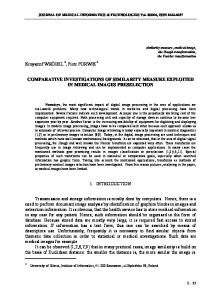
Hence, P ∗ , the solution to Eq. 2.2, maps the set S1 (P ∗ ) to the initial set S2 and since the motion is assumed to be global, P ∗ is an implicit solution to the image registration problem as no explicit similarity measure is used. Eq. 2.2 is solved using the intensity values of a single image, making the alignment process invariant to intensity changes. This process is presented in Figure 1.
Figure 1: The multi-sensor registration algorithm flow. Clockwise starting at the upper-left corner: the second image. The high-gradient pixel set S2 detected in the second image and overlayed on it. The set S2 is projected onto the other image using the initial estimate P 0 and named S1 . The global optimization process leads to the alignment of S1 .
4
2.3
Iterative optimization
Since F (S1 (P )) is a non-linear function of P , the motion parameters are computed by solving Eq. 2.2 using Newton’s iterative optimization method [10]. The iterative refinement equation is given by: ∇P Fn . P n+1 = P n + H −1 P
(2.4)
where ∇P Fn is the gradient vector of F in respect to P at iteration n ∇Fi =
h
∂F (xi ,yi ,) ∂P1
∂F (xi ,yi ) ∂P2
...
∂F (xi ,yi ) ∂Pm
and H nP is the Hessian matrix of F in respect to P at iteration n
n HP =
∂2F ∂P12 ∂2F ∂P2 ∂P1
∂2F ∂Pm ∂P1
∂2F ∂P1 ∂P2
...
∂2F ∂P1 ∂Pm
∂2F ∂P22
∂2F ∂P2 ∂Pm
.. .
... .. .
∂2F ∂Pm ∂P2
...
∂2F 2 ∂Pm
iT
(2.5)
.
(2.6)
In order to calculate ∇P Fn and H nP the derivative chain rule is used:
∂F (xi ,yi ) ∂Pj ∂F (xi ,yi ) ∂xi (xi ,yi , P n ) ∂F (xi ,yi ) ∂yi (xi ,yi , P n ) + = ∂x ∂Pj ∂y ∂Pj
∇P f (xi , y i ) =
∂∇P F (xi , y i ) ∂Pj ∂∇P F (xi , y i ) ∂xi (xi ,yi , P n ) ∂∇P F (xi , y i ) ∂yi (xi ,yi , P n ) = + . ∂x ∂Pj ∂y ∂Pj
H P (xi , y i ) =
(2.7)
(2.8)
where ∇F (xi , y i ) and H P (xi , yi ) are the gradient and Hessian in respect to Pj approximated at the ith pixel. P n is the parameters estimate after the nth iteration. Thus, ∇P Fn and H P are accumulated over the complete pixel set S1 (P ): ∇P Fn = and HP =
X
∇P Fn (xi , y i )
X
H P (xi , y i ) .
(xi ,yi )∈S1 (P )
(xi ,y i )∈S1 (P )
5
(2.9)
(2.10)
For motion models which are linear in respect to P n , such as the affine and projective models we have:
XAf f ine =
and
XPr ojective =
x y 1 0 0 0 0 0 0 x y 1
x y 1 0 0 0 x ex x ey 0 0 0 x y 1 x ey yey
The gradient vector and Hessian matrix can be expressed as:
∇P F n =
X
(xi ,y i )∈S1 (P )
.
Xi ∇(x,y) F n (xi , yi )
X
HP =
(2.11)
Xi H (x,y) XiT
(2.12)
(2.13)
(2.14)
(xi ,y i )∈S1 (P )
where ∇Fn and H are the gradient and Hessian in respect to the cartesian coordinate system: ∇Fn =
h
∂F (xi ,yi ) ∂x
H =
∂2F ∂x2 ∂2F ∂y∂x
∂F (xi ,yi ) ∂y
∂2F ∂x∂y ∂2F ∂y2
i
(2.15)
(2.16)
Eq. 2.4 is iterated until either of the following convergence criteria is met: 1. A maximal (predefined) number of iteration is reached. 2. The update of the parameters becomes smaller than a predefined size.
2.4
Multiscale extension
In order to improve the convergence properties of the iterative algorithm is section 2.3, a resolution pyramid is constructed. The alignment algorithm starts at the coarsest resolution scale of the pyramid, then follows the subsequent levels in a coarse-to-fine approach. At each resolution scale, the calculation described in Section 2 is conducted where the results of the calculation at each scale serves as an initial guess for the finer iteration scale. Finally, when the procedure stops at the finest resolution scale, the final motion parameters are obtained.
6
The coarse-to-fine refinement process allows the alignment process to lock on a single dominant motion even when multiple motions are present. This motion, which is named dominant motion, is essential due to the presence of outlier feature points.
3
Convergence properties
The convergence properties of the proposed algorithm resemble those of regular gradient methods [11]. Hence, a sufficient convergence condition can be derived by analyzing the properties of the iterative refinement term in Eq. 2.4: ∇P Fn ∆P n = H −1 P
(3.1)
where ∆P n is the iterative refinement at iteration n. which can be any positive-definite matrix, whose The convergence does not depend on H −1 P choice determines the convergence rate rather than the final values of the parameters.
3.1
Notation
Denote S E {S}
The set of pixels in I1 . The expectancy of pixels within S.
S1n
A subset of S - the set of pixels used at iteration n in I1 to evaluate Eq. 2.1.
n SDom
A subset of S1n , the set of pixels in S1n having large gradient values corresponding to true alignment.
n E {SDom }
n SDom
© n ª E SDom then
and
n The expectancy of pixels within SDom .
A subset of S1n , the set of pixels in S1n having small gradient values corresponding to false alignment. n . The expectancy of pixels within SDom n |SDom | , |S| ¯ ¯ n ¯ ¡ n ¢ ¡ ¢ ¯SDom n P SDom , P (x, y) ∈ SDom = , |S| n n P (SDom ) , P ((x, y) ∈ SDom )=
P (S1n ) , P ((x, y) ∈ S1n ) =
|S1n | . |S|
¯ ¯ n n n ¯ are the sizes of S, S n where |S|, |SDom | and ¯SDom Dom and SDom respectively. 7
(3.2) (3.3)
(3.4)
3.2
Estimation of the pixels sets expectancies
The expectancies of the sets can be estimated by
assuming
© n ª n n } P (SDom ) + E SDom (1 − P (SDom )) E {S} = E {SDom ¯ ¯ n ¯ © n ª |S| − ¯SDom |SDom | + E SDom = E {SDom } |S| |S| |S| À |SDom |
we get
(3.6)
© n ª E {S} ≈ E SDom
and
(3.7)
E {SDom } À E {S} .
3.3
(3.5)
(3.8)
Spatial gradient expectancies estimation
n The ratio of ESDom {∇Fn } and ES n
Dom
{∇Fn } can be estimated by approximating the derivative
∇F is using finite differences E {∇F (x, y)} = E
½
∂F ∂F , ∂x ∂y
¾
(3.9)
where © ∂F ª ' E {F (x, y)} − E {F (x − 1, y)} n ∂x o ' E {F (x, y)} − E {F (x, y − 1)} E ∂F ∂y E
n In particular, the expectancies ESDom {∇Fn } and ES n
Dom
and 3.10
(3.10)
{Fn } can be estimated using Eqs. 3.7, 3.8
© ∂F ª |(x, y) ∈ S ' E {SDom } − E {S} À 0 Dom o n ∂x ∂F E ∂y |(x, y) ∈ SDom ' E {SDom } − E {S} À 0, E
(3.11)
n set we get while for the SDom
E E Hence,
© ∂F n ∂x ∂F ∂y
¯ ª © n ª ¯(x, y) ∈ S n Dom o ' E SDom − E {S} ≈ 0 ¯ © n ª ¯(x, y) ∈ S n Dom ' E SDom − E {S} ≈ 0 n ESDom {∇Fn } À ES n
Dom
8
{∇Fn }
(3.12)
(3.13)
3.4
Convergence condition
n n By decomposing ∇F n according to the ith pixel’s relation to either SDom or SDom we get
∇P F
X
=
(xi ,yi )∈S(P )
X
=
Xi ∇Fn (xi , yi )
n (xi ,yi )∈SDom
Xi ∇Fn (xi , yi ) +
X
n (xi ,yi )∈SDom
Xi ∇Fn (xi , yi )
(3.14)
= ∇P FnDom + ∇P FnDom where ∇P FnDom and ∇P FnDom correspond to dominant and non-dominant pixel sets respectively. © ª Next we calculate E ∇P Fn , the expectancy of ∇P F : ª © = E ∇P Fn
X
n (xi ,yi )∈SDom
E {Xi ∇Fn (xi , yi )} +
X
= E {Xi }
n (xi ,yi )∈SDom
X
n (xi ,yi )∈SDom
E {∇Fn (xi , yi )} +
E {Xi ∇Fn (xi , yi )}
X
n (xi ,yi )∈SDom
³ ¯ ¯ n n ¯E n n | ESDom {∇Fn } + ¯SDom = E {Xi } |SDom S
Dom
(3.15)
E {∇Fn (xi , yi )}
´ {∇Fn }
n n and SDom are assumed to be similar and independent of the and the spatial distributions of SDom
gradient values. Therefore, the convergence condition is given by: ¯ ¯ n n ¯E n n | ESDom {∇Fn } À ¯SDom |SDom S
Dom
{∇Fn }
(3.16)
By substituting Eq. 3.13 into Eq. 3.16 we get that convergence is achieved for: ¯ ¯ n n ¯ | > ¯SDom |SDom
(3.17)
We conclude that the iterative optimization scheme converges when the initial estimate used, provides registration of a small part of the chosen pixels set S2 to its true S1 locations. The size of the initially aligned set, is given by: n n | À (|S1 | − |SDom |) |SDom
ES n
Dom
{∇Fn }
(3.18)
n ESDom {∇Fn }
Hence, n | À |S1 | |SDom
ES n
Dom
ES n
Dom
{∇Fn }
n {∇Fn } + ESDom {∇Fn }
9
≈ |S1 |
ES n
Dom
{∇Fn }
n ESDom {∇Fn }
(3.19)
The smaller the ratio in intensity expectancies
ES n
Dom
ES n
Dom
{∇Fn }
{∇Fn } ,
n the smaller the set |SDom | to be used.
Thus, the sharper the image used for the iterative optimization, the larger the convergence range.
4
Experimental results
Several image pairs acquired by medical and remote sensing applications were registered using an affine and projective parametric motion models. In order to demonstrate the alignment, the high-gradient magnitude pixel set was overlayed on both images, where the initial estimate of the motion is given by its pixel overlay. A linear multi-resolution pyramid (Section 2.4) with 3 scales was used. Figure 2 shows the registration of medical multi-modality images using an affine motion model. These images are characterized by low noise and sharp contrast between the dominant and non-dominant sets. Thus, according to Eq. 3.19 these images can be registered using a small set of n and a less accurate initial estimate. Figure 3 shows the affine corresponding dominant pixels SDom
registration results of the severely dissimilar and noisy multi-sensor images, in this case, the ratio ES n
{∇Fn } Dom ES n {∇Fn } Dom
is not small due to the presence of non-mutual image features and thus, a relatively
accurate initial estimate is needed. The registration results of these images, using the projective motion model are presented in Figure 4. The images in Figure 5 are taken from [3]. In this scenario there is a small number of non-mutual image feature, but the estimated motion is large.
5
Discussion
In this work a robust multi modality image registration algorithm was presented. The algorithm uses an implicit geometrical similarity measure which is invariant to intensity dissimilarities. The registration is achieved by tracking the migration of high-gradient pixels using robust global optimization. The convergence analysis leads to the derivation of an analytic convergence criterion. The experimental results demonstrate the effectiveness of the proposed algorithm by registering real multisensor and multi-modality images.
References [1] W. M. Wells III, P. Viola, H. Atsumi, S. Nakajima, and R. Kikinis, “Multi-modal volume registration by maximization of mutual information”, Med. Image Anal., vol. 1, no. 1, pp. 35-51, 1996.
10
(a)
(b)
(d)
(c)
Figure 2: Registration results of CT and MRI multi-modality images using the affine motion model: (a) original MRI image overlayed with the set of high-gradient pixels . (b) Initial estimate of the overlayed set in the CT image. (c) Composite image. (d) Final alignment of the pixel set after migration. [2] Josien Pluim, J. B. Maintz and M.Viergever. “Image Registration by Maximization of Combined Mutual Information and Gradient Information”, IEEE Transactions on Medical Imagining, VOL. 19, NO. 8, August 2000. [3] M. Irani and P. Anandan, “Robust Multi-Sensor Image Alignment”. IEEE International Conference on Computer Vision (ICCV), India, January 1998. [4] H. Li, B.S. Manjunath, and S.K. Mitra, “A Contour Based Approach to Multisensor Image Registration”, IEEE Trans. Image Processing, vol. 4, pp. 320-334, March 1995. [5] J. Maintz, M. Viergever, “An Overview of Medical Image Registration Methods”, ftp://cs.uu.nl/people/twan/brussel_bvz.pdf [6] M.
Irani
and
P.
Anandan.
“All
About
ftp://ftp.robots.ox.ac.uk/pub/outgoing/phst/summary.ps.gz . 11
Direct
Methods”,
(a)
(b)
(d)
(c)
Figure 3: Registration results of SAR and FLIR multi-sensor images using the affine motion model: (a) original SAR image overlayed with the set of high-gradient pixels . (b) Initial estimate of the overlayed set in the FLIR image. (c) Composite image. (d) Final alignment of the pixel set after migration. [7] L. Brown, “A survey of image registration techniques”, ACM Computer Surveys, vol. 24(4), pp. 325-376, 1992. [8] R. Sharma and M. Pavel, “Registration of video sequences from multiple sensors” in Proceedings of Image Registration Workshop, Publication CP-1998-206853, NASA-GSFC, November 1997. [9] A. Guziec, X. Pennec, N. Ayache “Medical Image Registration Using Geometric Hashing”, IEEE Computational Science and Engineering, October-December 1997 (Vol. 4, No. 4), pp. 29-41. [10] P. Gill , “Practical Optimization”, Academic Press, 1982. [11] A. Averbuch, Y. Keller, “Fast motion estimation using bidirectional gradient methods”.
12
(a)
(b)
Figure 4: Registration results of SAR and FLIR multi-sensor images using the projective motion model: (a) Composite image. (b) Final alignment of the pixel set after migration. The initial pixel set and its initial projection are the same as in Figure 4. [12] E. Simoncelli and E. Adelson, “Noise removal via Bayesian wavelet coring”, 3rd IEEE Int’l Conf on Image Processing. Laussanne Switzerland, September 1996.
13
(a)
(b)
(d)
(c)
Figure 5: Registration results of EO and IR multi-modality images presented in [3] using the affine motion model: (a) original IR image overlayed with the set of high-gradient pixels . (b) Initial estimate of the overlayed set in the EO image. (c) Composite image. (d) Final alignment of the pixel set after migration.
14