University of Hertfordshire Business School .... the historical notes below. ..... Fitting linear relationships: A history of the calculus of observations 1750-1900.
THE UNIVERSITY OF HERTFORDSHIRE BUSINESS SCHOOL WORKING PAPER SERIES The Working Paper series is intended for rapid dissemination of research results, work-inprogress, innovative teaching methods, etc., at the pre-publication stage. Comments are welcomed and should be addressed to the individual author(s). It should be remembered that papers in this series are often provisional and comments and/or citation should take account of this. For further information about this, and other papers in the series, please contact: University of Hertfordshire Business School College Lane Hatfield Hertfordshire AL10 9AB United Kingdom
©C. Tofallis
Multiple Neutral Regression Dr. C. Tofallis Operational Research Paper 14 UHBS 2000:13
1
MULTIPLE NEUTRAL REGRESSION
Presented at the APMOD 2000 conference.
DR. CHRIS TOFALLIS
2
MULTIPLE NEUTRAL REGRESSION
Abstract
We present a multiple regression fitting method which, unlike least-squares regression, treats each variable in the same way. It can be used when seeking an empirical relationship between a number of variables for which data is available. It does not suffer from being scale-dependent − a disadvantage of orthogonal regression (total least squares). Thus changing the units of measurement will still lead to an equivalent model − this is clearly important if a model is to be meaningful. By formulating the estimation procedure as a fractional programming problem, we show that the optimal solution will be both global and unique. For the case of two variables the method has appeared under different names in different disciplines throughout the twentieth century: as the reduced major axis or line of organic correlation in biology, as Stromberg's impartial line in astronomy, and as diagonal regression in economics (in which field two Nobel laureates have published work on the method). We gather together the most important results already established.
Introduction The method of regression is undoubtedly one of the most widely used quantitative methods in both the natural and social sciences. For most users of the technique the term is taken to refer to the fitting of a function to data by means of the least squares criterion. Researchers who probe further into the field will discover that other criteria exist, such as minimising the sum of the absolute deviations, or minimising the maximum absolute deviation. All of these fitting criteria have one thing in common: they measure goodness of fit by referring to deviations in the dependent variable alone. If one is intending to use the regression model for the purpose of predicting the dependent variable then this is a natural track to follow. If, however, one is seeking the underlying relationship between a number of variables then
3
there may not be an obvious choice for the dependent variable. One would then be interested in a method which treated all variables on the same basis. This is the underlying motivation for this paper. We allow that there may be both natural variation and/or measurement error in all of the variables (another departure from conventional regression). We do not assume that we have information on error variances (these are rarely known) or the error distributions associated with the data. (If such information is available then there is an established statistical approach known as errors-in-variables, see Cheng and Van Ness, 1999.) In fact we are simply presenting an estimation procedure without any distributional assumptions. We justify our choice of method by virtue of certain useful properties which other methods do not possess.
Total least squares or orthogonal regression Suppose we wish to fit a line to data, but without basing it solely on the vertical deviations from the line. A possible alternative fitting criterion that one might consider is to minimise the sum of the perpendicular distances from the data points to the regression line, or the squares of such distances. This involves applying Pythagoras' theorem to calculate such distances and so involves summing the squared deviations in each dimension. This is therefore sometimes referred to as 'total least squares', as well as 'orthogonal regression'. The trouble with this approach is that we shall be summing quantities which are in general measured in different units; this is not a meaningful thing to do. One can try to get around this objection by normalising in some way: e.g. divide each variable by its range, or its standard deviation, or express it as a percentage of some base value, etc. Unfortunately each of these normalisations results in a different (or non-equivalent) fitted model for a given set of data. It is also worth noting that even if a variable is dimensionless, multiplying it by some constant factor will also affect the resulting model. This is because total least squares will tend to concentrate on reducing the deviations of that variable whose values happen to be greater in absolute magnitude, effectively attaching greater weight to it. Ideally we would like a method that was invariant to a scale change in any of the variables. For more on total least squares see Van Huffel and Vandewalle (1991) and Van Huffel (1997).
4
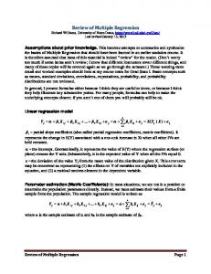
The multiplicative approach Instead of adding deviations in each variable let us multiply them together. In other words for each data point multiply together the deviations from the fitted line for each variable. Thus in the two variable case we multiply the vertical (y) deviation with the horizontal (x) deviation. This gives twice the area of the triangle described by the data point and its projections (parallel to the axes) onto the regression line. Our fitting criterion is then to minimise the sum of these triangular areas, i.e. the sum of the products of the deviations in each variable. Woolley (1941) refers to these triangles as 'area deviations'. See Figure 1.
Figure 1 There are four data points: one at each right angle of the shaded triangles. The aim is to fit a line such that the sum of the triangular areas is minimised.
This idea is not new; in fact it has surfaced in many fields over the twentieth century. (See the historical notes below.) Unfortunately it has usually appeared under different names in each discipline and this may have played a part in it not being more widely known − there
5
have been small pockets of scattered usage and a critical mass of unified literature has yet to be achieved. One of the attractions of this method is that it produces the same model irrespective of which variable is labelled x and which is labelled y; this symmetry is apparent from the fact that if we exchange the axes on which each variable is plotted, the triangular areas remain the same − triangles that were above the line now appear below, and vice versa − we have reflected everything through the line y = x. For an algebraic proof see Woolley (1941). Because no variable is given special treatment, we choose to call this approach 'neutral regression'. Note also that this method is invariant to scale change for any variable, since if we scale up one variable by some factor then we are merely stretching the length of the triangles in that dimension − the total triangular area is scaled up by the same factor. In fact the entire graph is simply stretched in one of the dimensions with everything remaining in the same relative position. Relation to least squares regression: the geometric mean property Consider the least squares regression lines of y on x, and x on y plotted using the same axes. They each pass through the centroid of the data (the point whose co-ordinates are the means of the variables), but in general they will have different slopes and intercepts. The neutral regression model will also pass through the centroid, but possesses the attractive property of having a slope (and intercept) lying somewhere between those of the two least squares lines: in fact it will have a slope that is the geometric mean of these two. It is for this reason that the resulting model is sometimes referred to as the geometric mean functional relation. This connection has been made at different times in different disciplines (e.g. see Barker, Soh, and Evans (1988) for a proof).
Properties of neutral regression Paul Samuelson (1942) lists seven 'properties which a method of determining regression equations might desirably possess'. He states (without providing any justification) that one of these is in principle impossible except when the correlation is perfect. The desirability of another of his properties is open to question: namely that the fitted equation should be invariant under any orthogonal transformation of variables (i.e. transformations that leave
6
angles and lengths unchanged). Such transformations include rotation of the axes: thus a real relationship represented by a line that passed through the origin (such as y = x) could be transformed into a non-existent relationship by rotating in such a way that the fitted line coincided with the x or y-axis. This does not therefore seem to be a useful property for a fitting procedure to possess. However what is particularly remarkable is that Samuelson proves that what we here call neutral regression is the only method which satisfies all of his desirable properties, bar the two we have mentioned. His list includes invariance under scale change, invariance under interchange of variables, and reduction to the correct equation for perfectly correlated variables. Kruskal (1953) also proved a uniqueness theorem: of all the procedures which depend only on first and second moments (i.e. on the means, covariance and standard deviations), neutral regression is the only line-fitting procedure which behaves correctly under translation and change of scale. This implies that any linear transformation on any variable is acceptable. The translation invariance is easy to visualise since adding a constant to say, the y-variable, merely shifts the data points en masse in the vertical direction, hence the triangular areas are unaffected. As for the scale invariance: imagine multiplying all the values of one of the variables, say y, by some constant, this would stretch the plane containing the data points in the y-direction; the height and hence the area of each triangle would be multiplied by the same factor whilst the x-deviation (the width of each triangle) would be unaffected. Hence the slope of the 'least areas line' would scale by the same factor, and hence is scale invariant. The simple geometry of our fitting criterion allows us to see that these arguments extend to higher dimensions and so will apply for the case of multiple regression.
Comparison with other line-fitting methods Babu and Feigelson (1992) noted that "For many applications…only a set of correlated points is available to fit a line. The underlying joint distribution is unknown, and it is not clear which variable is 'dependent' and which is 'independent'." They compared a number of line-fitting techniques and proved the following theorem: whenever the fitting techniques are applied to the same set of data, the estimated slopes will generally differ, with the two extremes provided by the ordinary least squares (OLS) regressions (y regressed on x, and x
7
on y). In between these will lie the slopes obtained from orthogonal regression and the OLS bisector (the line which bisects the angle formed by the two least squares lines). And nested in between the latter will be the slope value obtained by neutral regression (which they refer to as the 'reduced major axis' or RMA); i.e. the neutral regression slope provides the median value from these five fitting techniques. Their paper also includes a useful table providing expressions for the variance of the slope estimate for each technique. Babu and Feigelson also applied the techniques to simulated data using a Monte Carlo approach. They ran 500 simulations for each method using a large data sample (500 points), and a further 500 simulations using a smaller data sample (50 points). These were repeated under a variety of conditions of correlation and standard deviation. They were interested in how accurately the theoretical slope could be reproduced. They found that orthogonal regression consistently gave the poorest accuracy, and that taking the mean of the two OLS slopes gave intermediate accuracy. The RMA (neutral regression) and OLS bisector gave the highest accuracy. In their conclusion however, they reject RMA on the grounds that the expression for the slope does not depend on the correlation between x and y. This is rather a strange objection because the correlation is a measure of the strength of the linear relationship and should be independent of the slope. The slope provides an estimate of the rate of change of y with x; why should this value be determined by the correlation (r)? After all, two regression lines can have the same slope but the data sets on which they are based can differ in the correlation; conversely, two sets of data can have the same correlation but have different regression slopes. It is conceivable that their objection may be grounded in the 'OLS conditioning' that most researchers are imbued with (since in OLS the slope is related to the correlation (r), according to: slope = r sy/sx ). The eminent statistician John Tukey has indeed described least squares regression as a statistical idol and feels "it is high time that it be used as a springboard to more useful techniques" (Tukey, 1975). Another connection between OLS and correlation is that r2 = [slope of OLS(y on x)] / [Slope of OLS(x on y)] where y is plotted on the vertical axis for both cases so that the slope represents the rate of change of y with x.. This implies that for a data set with a correlation of 0.7 the usual OLS regression line will have a slope which is less than half the magnitude of the OLS regression of x on y. In general the lower the correlation the more these two lines will diverge, irrespective of what the 'true' underlying relationship is. This
8
dependence on correlation may partly explain why the two OLS lines provide the extreme values when the slopes are placed in order for the five methods mentioned above. If the 'true' slope lies somewhere between the two least squares estimates then the usual OLS slope provides an under-estimate for the absolute value and the OLS (x on y) an overestimate. Riggs et al (1978) make the point forcefully: "OLS continues to be by far the most frequently used method even when it is obviously inappropriate. As a result, hundreds if not thousands of regression lines with too-small slopes are being published annually". Riggs, Guarnieri and Addelman (1978) managed to come up with a staggering number (34) of different line-fitting methods−admittedly many were variations which involved different weighting schemes. They rejected 16 of them due to deficiencies such as lack of scaleinvariance, and carried out a Monte Carlo study of the remaining 18 methods to see how well they could reproduce the true underlying model which was used to generate the data. Their conclusion is couched in terms of λ, the ratio of the error variance in the y variable to the error variance in the x variable: "In overall performance, judged both by root mean square error and percent bias, the geometric mean [i.e. neutral regression] was almost always the best method when λ =1…For λ < 1 error-weighted methods, and for λ >1 variance-weighted methods tended to be superior." Unfortunately λ is rarely known because it "requires special observations on y when x is accurately known, and on x when y is accurately known" (Ricker, 1973). After some discussion about what to do when λ is not known, Ricker comes to the "conclusion that the geometric mean regression is the best available estimate of the functional relationship for the situation where all the variability of both variates is due to measurement error and there is no supplementary information concerning the relative point errors in x and y". Ricker also argues for the use of this method when the variability in each variable is largely or entirely natural rather than due to measurement error. Hence he recommends its use in biological work.
Multiple neutral regression (MNR) So far we have seen that neutral regression possesses a number of desirable theoretical properties, and that comparative simulations with other fitting methods show it to perform well in many situations. This provides us with the motivation to extend the method to the case of multiple variables. We shall do this by generalising the concept of area deviations as
9
shown in Figure 1. From each point we extend a line to the fitted plane in a direction parallel to the co-ordinate axes; in three dimensions this will describe a tetrahedron with a right angle at the data point. The volume of this tetrahedron corresponds to the 'volume deviation' for that data point. We then fit a plane to the data such that the sum of volume deviations (V) is a minimum. The same idea carries over into higher dimensions when fitting a hyperplane. Draper and Yang (1997) have also presented work on multiple regression which treats each variable on the same footing. Their approach differs from ours in that they minimised the sum of the geometric means of the squared deviations in each dimension. This quantity is also related to the volume deviations, and corresponds, in n dimensions, to minimising the sum of quantities of the form V2/ n . Indeed we can propose a whole family of fitting methods in which one minimises Σ VP where higher values of p are chosen to emphasise the larger deviations. This is akin to the family of fitting procedures based on Lp norms where p = 1 corresponds to minimising the sum of the absolute y-deviations (known as LAV or least absolute value regression), p = 2 corresponds to OLS, and p = ∞ is the Chebyshev or minimax norm where one minimises the largest residual.
Estimation procedure Given that we are aiming to minimise a certain quantity (Σ V), it is natural to formulate the problem as one of optimisation. To make matters easier to visualise we first describe the three dimensional case. We shall fit a plane of the form: ax + by + cz = k
(1)
The coefficients or parameters are best understood by noting that this plane intersects the axes at x = k/a, y = k/b, and z = k/c respectively. Let us consider the extreme values of the parameters: If, say, b = 0 then the plane is parallel to the y-axis and so there is no dependence on y. An infinite value for b corresponds to a plane perpendicular to the y-axis, and so once again there is no dependence on the y variable. We shall assume that we do not have such cases, or that the relevant variable is removed from the data set if they do arise. Note that k = 0 corresponds to the plane passing through the origin, which is perfectly acceptable.
10
We can of course multiply through equation (1) by any non-zero factor to obtain an equivalent form. So we can impose one constraint on the parameters to specify a single solution; for instance we might choose the constraint to be a+b+c=1
(2)
or if one did not expect the plane to pass through the origin, one could instead set k = 1. Consider any data point with co-ordinates (xi , yi , zi ), the associated volume deviation is the volume of the tetrahedron whose sides are the deviations in the x, y, and z directions. From geometry the volume of such a right-angled tetrahedron is given by one sixth the product of the base, height, and width. From (1) the deviation in the x-direction of the data point from the plane is given by: xi − (k − byi − cz i) / a
or
(axi + byi + czi − k ) / a
Similarly the deviations in the y and z directions are: yi − (k − axi − cz i) / b or and zi − (k − axi − by i) / c
(axi + byi + czi − k ) / b or (axi + byi + czi − k ) / c
Hence the volume deviation associated with this data point is proportional to | (axi + byi +czi
− k ) 3 / (abc) | The optimisation problem is thus to choose values of the parameters a, b, c, k so as to minimise Σ | (axi + byi + czi − k ) 3/ (abc) |
(3)
If instead of three variables, we have n variables, then this objective function generalises in the obvious way. Properties of the solution: optimality and uniqueness By formulating the above optimisation problem as a certain type of non-linear programme we can show that the solution possesses some useful properties.
11
In order to deal with the absolute value operator in (3) we can define non-negative variables u and v: ui − vi = axi + byi + czi − k The pairs of non-negative quantities ui , vi are a type of residual: those points with a positive u value lie on the opposite side of the fitted plane to those with a positive v value. Note that the minimisation will ensure that at least one of each pair (ui , vi ) will be zero. Next, without loss of generality we shall assume that each of the fitted coefficients (a, b, c) is positive; this can always be arranged by multiplying the values of any variable by −1 wherever necessary, and corresponds to axis-reversal. The optimisation problem (3) then becomes minimise
(Σ ui 3 + vi 3) / (abc)
(4) subject to
ui − vi = axi + byi + czi − k ui , vi ≥ 0 and a + b + c = 1
We have now succeeded in formulating the problem as a particular type of fractional programming problem. The objective function is a ratio of functions with the numerator being non-negative and strictly convex and the denominator being concave and positive. This implies the objective function is strictly explicit quasi-convex (see page 56 of StancuMinasian, 1997). The constraints in (4) define a convex set, this in turn implies that the any local minimum will be a global minimum, and furthermore that it will be unique (by Theorems 2.3.5 and 2.3.6 respectively, in Stancu-Minasian, 1997). Clearly both of these properties are retained in higher dimensions i.e. when we have more than three variables. These are very valuable properties as it means that we can employ general-purpose optimisation software to seek the solution. In particular this includes the solvers which are built in as standard in spreadsheet packages, hence the wider community can employ our method.
12
Historical notes Before concluding we here bring together from various disciplines some of the appearances of the technique for the case of two variables. An early reference is that of Teissier (1948); however the presence of a paper written in French in an English-language journal could not have helped its dissemination. A paper in English appeared soon after (Kermack and Haldane, 1950) in which the fitted line was referred to as the 'reduced major axis'. Both of these dealt with allometry, which is that branch of biology which studies the relative size and growth of one part of an organism relative to another part. In such investigations there will be variability in both measurements and there is usually no clear candidate for selecting one of the variables as being 'dependent' and the other 'independent'. As a result the method was later strongly advocated for use in fishery research and biology in general by Ricker (1973). In biology the resulting line is also called the 'line of organic correlation' (e.g. Kruskal, 1953). Astronomy has always been a fruitful area for new quantitative techniques. Indeed the least squares method was introduced to deal with the orbits of heavenly bodies by Laplace, Legendre and Gauss in the early 1800's. (See the book by Farebrother (1999) for a history of fitting procedures prior to 1900.) The method which we have been discussing appeared in the astronomical literature in 1940 (Stromberg) hidden in a paper entitled 'Accidental systematic errors in spectroscopic absolute magnitudes for dwarf GoK2 stars'. It was subsequently referred to as 'Stromberg's impartial line'. In cosmology Feigelson and Babu (1992) note that 'accurate regression coefficients are crucial to measuring the expansion rate of the universe, estimating the age of the universe, and uncovering large-scale phenomena such as superclustering'. The more distant a galaxy, the faster it moves away from us, but one cannot say that that the speed depends on distance or vice versa, hence the need for a method that treats variables symmetrically. They also mention calibration problems where 'one instrument or measurement technique is calibrated against another, with neither one being inherently a standard'; both measurement error and intrinsic scatter about the line are present. Another field where our technique has been discussed is in economics. Woolley (1941) introduces it as 'the method of minimised areas'. Samuelson (1942) then commented that "this is nothing other than Frisch's 'diagonal regression'" and gives a reference dating back to
13
1934. However the earliest of all references appears to have been found by Ricker (1975) who cites a German paper on meteorology going back to 1916 (Sverdrup). Conclusion We have considered the situation where we wish to estimate a relationship between variables where the data for each variable is treated on the same basis. We may wish to do this rather than use conventional least squares regression for a number of possible reasons. For instance, it may not be obvious which variable is the dependent variable (possibly because all the variables are the effects of a common cause which has not or cannot be measured), or all the variables have uncertainty associated with them and no information is available regarding the error variance so that the errors-in-variables approach cannot be used. When only two variables are involved we have seen that work has been done to compare various techniques for estimating an underlying relationship, and that the technique which we here call neutral regression has shown itself to be desirable for a number of reasons. Analytically, it has been shown that it is units-invariant, as well as being invariant to linear transformation of either or both of the variables. It has also been demonstrated that it will always provide a slope value which lies between those given by the two OLS lines. The two OLS slopes will increasingly diverge as the correlation in the data falls, whereas with neutral regression the slope value is independent of the correlation. Numerical simulations also show that our technique is very good at unearthing the true underlying model. In the light of these useful properties and what Draper and Smith (1998) call its 'appealing natural symmetry', there was clearly a case for extending the method to the case of multiple variables. We did this by generalising the notion of area deviation to that of volume and hyper-volume deviations. We chose this avenue rather than that of the geometric mean property to ensure that the invariance properties are retained. Generalising the geometric mean property would involve taking all possible least-squares regressions (taking each variable in turn to be dependent), and then estimating each coefficient as the geometric mean of the relevant coefficients from all the regressions. Whether that would also possess the same invariance properties remains to be seen. Note that this is not what Draper and Yang (1997) did, rather they took the geometric mean of squared deviations in each
14
dimension; they showed that their solution for the coefficients is a convex combination of the separate least squares solutions. Much work needs to be done to explore the method we have proposed. We intend to carry out Monte Carlo simulations to see how well it reproduces the underlying model in comparison with other fitting procedures. Another challenge is to obtain a closed form expression for the coefficients. Recently, the presentation of the method for two variables (under the name 'geometric mean functional relationship') in the latest edition of the widely known monograph on regression by Draper and Smith (1998) will hopefully do much to raise interest in a wider audience, particularly statisticians. The fact that most of the literature on the subject has appeared in the natural and social sciences is testament to its utility. It is however surprising that the statistical community has largely been unaware of this elegant and valuable technique. It is also noteworthy that it has attracted the attention of eminent researchers such as Kruskal and J.B.S.Haldane, as well as Nobel prizewinners (Samuelson and Frisch), this too must commend its further investigation in higher dimensions.
15
References Babu, GJ and Feigelson, ED (1992). Analytical and Monte Carlo comparisons of six different linear least squares fits. Communications in Statistics: Simulation and Computation, 21(2), 533-549. Barker, F, Soh, YC, and Evans, RJ (1988). Properties of the geometric mean functional relationship. Biometrics 44, 279-281. Belsley, DA (1991). Conditioning Diagnostics. Wiley, New York. Cheng, C-L and Van Ness, JW (1999). Statistical regression with measurement error. Arnold, London. Draper, NR and Smith, H (1998). Applied regression analysis (3rd edition). Wiley, New York. Draper, NR and Yang, Y (1997). Generalization of the geometric mean functional relationship. Computational Statistics and Data Analysis, 23, 355-372. Farebrother, RW (1999). Fitting linear relationships: A history of the calculus of observations 1750-1900. Springer, New York. Feigelson, ED, and Babu, GJ (1992). Linear regression in astronomy II. Astrophysical J. 397, 55-67. Frisch, R (1934) Statistical confluence analysis by means of complete regression systems. University Institute of Economics, Oslo. Kermack, KA, and Haldane, JBS (1950). Organic correlation and allometry. Biometrika, 37, 30-41. Kruskal, WH (1953) On the uniqueness of the line of organic correlation. Biometrics 9, 47-58. Ricker, WE (1973). Linear regressions in fishery research. J. Fisheries Research Board of Canada 30, 409-434.
16
Ricker , WE (1975). A note concerning Professor Jolicoeur's comments. J. Fisheries Research Board of Canada 32, 1494-1498. Riggs, DS, Guarnieri, JA and Addelman, S (1978). Fitting straight lines when both variables are subject to error. Life Sciences 22, 1305-1360. Samuelson, PA (1942). A note on alternative regressions. Econometrica 10(1), 80-83. Stancu-Minasian, IM (1997). Fractional Programming: Theory, Methods and Applications. Kluwer Academic, Dordrecht. Stromberg, G (1940). Accidental systematic errors in spectroscopic absolute magnitudes for dwarf GoK2 stars. Astrophysical J. 92, 156ff. Sverdrup, H (1916). Druckgradient, wind und reibung an der erdoberflache. Ann. Hydrogr. u. Maritimen Meteorol. (Berlin) 44, 413-427. Teissier, G (1948). La relation d'allometrie: sa signification statistique et biologique. Biometrics 4(1), 14- 48. Tukey, JW (1975). Instead of Gauss-Markov least squares, what? In Applied Statistics ed. Gupta, RP. North-Holland Publishing. Van Huffel, S (1997). Recent advances in total least squares. SIAM, Philadelphia. Van Huffel, S and Vandewalle, J (1991). The total least squares problem: Computational aspects and analysis. SIAM, Philadelphia. Woolley, EB (1941). The method of minimized areas as a basis for correlation analysis. Econometrica 9(1), 38-62.
17
Further work and challenges Is there a closed-form expression for the coefficients, possibly derivable using calculus? Do the coefficients agree with the application of the geometric mean to higher dimensions? Much simulation with data sets needs to be carried out to see how well our approach reproduces the known underlying coefficients. Note that when correlation is high different methods will tend to agree closely in the case of two dimensions. Does the approach help with problems associated with multicollinearity? The mathematical programming formulation may provide useful information from the associated sensitivity analysis/dual programme. Prove that the model passes through the centroid of the data.
Numerical example We have taken two data sets ( A and B) from Belsley (1991, page 5) that were generated from the equation y = 1.2 − 0.4 x1 + 0.6 x2 + 0.9 x3 + ε
(5)
where ε is normally distributed with mean zero and variance 0.01 . Given that the underlying error distribution is normal we will compare our procedure with conventional least squares (OLS). The largest absolute correlation between variables on the right hand side was 0.61 . For data set A OLS produces the model y = 1.255 + 0.974 x1 + 9.022 x2 − 38.44 x3
with R2 = 0.992.
whilst MNR gave: y = 1.200 − 0.4345 x1 + 0.371 x2 + 1.970 x3
18
Let us compare results with the true model (5): OLS gives the wrong order of magnitude for the x2 coefficient and even more seriously gives the wrong sign for the coefficients of the other two variables. By contrast MNR has the right order of magnitude for the x2 coefficient and also has the correct sign for both of the other two parameters. Now for data set B: OLS:
y = 1.275 + 0.247 x1 + 4.511 x2 − 17.644 x3
MNR: y = 1.199 − 0.435 x1 + 0.371 x2 + 1.979 x3 Once again MNR is superior on all the parameters. It is worth pointing out that the two data sets were very similar: the difference was never more than one in the third digit for the x-variables and the y column was the same for both sets. Yet the two OLS fits give widely differing parameters. The two MNR fits however are very similar indeed. Hence there is evidence here that MNR is a robust method which is not sensitive to small changes in the data. Clearly extensive simulations need to be carried out to establish the worth of MNR. This will be the subject of a future paper. But if the behaviour in two dimensions is found to carry over into the multiple variable case then we shall have a very valuable technique for seeking the underlying model from a given set of data.
19