Multiresolution transforms in modern image and video ... - Microsoft

Multiresolution transforms in modern image and video coding systems Henrique S. Malvar Microsoft Research, One Microsoft Way, Redmond, WA 98052 ABSTRACT This paper presents a brief overview of the multiresolution transform designs used in a few image and video compression systems, namely H.264, PTC (progressive transform coder), and JPEG2000. The first two use hierarchical transforms, and the third uses wavelet transforms. We review the basis constructions for the hierarchical transforms, and compare some of their characteristics with those of wavelet transforms. In terms of compression performance as measured by peak-signal to noise ratio, H.264 provides the best performance, but at much higher computational complexity. In terms of visual quality, the multiresolution transforms provide an improvement over block (single resolution) transforms. Keywords: wavelet transforms, lapped transforms, hierarchical transforms, image coding, video coding.

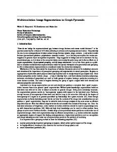
1. INTRODUCTION Compression of natural images (pictures) and video is quite common today; for example in Web pages we usually find images compressed with the JPEG (Joint Photographic Experts Group) codec (coder/decoder) [1] and video compressed with several kinds of MPEG (Moving Picture Experts Group) codecs [2]. A fundamental approach towards compression of media signals is to remove redundancy via signal prediction or linear transforms (or a combination of both), followed by a quantization (scaling and rounding to a nearest integer) and entropy coding (representing those integers with a small number of bits by exploiting their joint statistics) [3]. The scaling factor in the quantization process controls the basic tradeoff between compressed file size and decoded signal fidelity. In Fig. 1 we show a basic diagram representing the processing steps of a modern image or video compression that uses those ideas. By cascading a pixel-domain predictor with a transform operator, we mean that the transform is computed on the prediction residuals. The color space mapper is a first step of redundancy reduction, usually converting the pixels from an R-G-B color space to a luminance and chrominance space, such as Y-Cb-Cr (luma, blue-luma, and red-luma), with the luma and chroma images typically being encoded independently. For video coding, pixel prediction is usually nonlinear, through motion compensation – a motion field applied to a previously-encoded frame [2,4]. In image coding, most codecs do not use pixel prediction, so that a linear transform is applied directly to the image pixels. A notable exception is the new H.264 (also referred to as MPEG-4 Part 10) video codec [4], in which “intra” frames (those encoded independently, that is, without motion-based prediction from other frames) use pixel prediction from previously-encoded blocks within the same frame. We discuss this aspect further in Section 3. PREVIOUSLYENCODED DATA ORIGINAL IMAGE

COLOR SPACE MAPPING

QUANTIZATION

PIXEL-DOMAIN PREDICTION

BLOCK GROUPING

ENTROPY CODER

MULTIRESOLUTION TRANSFORM

ENCODED IMAGE

Figure 1. Simplified block diagram of a typical image or video compression system.

2. MULTIRESOLUTION TRANSFORMS Implicit in the diagram in Fig. 1 is that the transform operator is not applied to the image as a whole, but rather to blocks of pixels. In codecs such as JPEG [1] or MPEG [2], the blocks have the fixed size ox 8×8, and the transform is a DCT (discrete cosine transform). Other transforms can be used, but the DCT is fast-computable and is nearly optimal in terms of energy compaction [3,5], that is, for typical blocks the low-frequency coefficients have high magnitudes, whereas the high-frequency coefficients have low magnitudes. After quantization, many of the high-frequency coefficients are truncated to zeros, which are efficiently compressed by the entropy coder. The choice of block size is determined by a basic tradeoff: larger blocks are better for encoding flat regions, but small blocks lead to fewer ringing artifacts due to the missing high-frequencies [5,6]. The sets of pixels that form the blocks can be either disjoint (non-overlapping), as in JPEG or MPEG, or overlapping, as in wavelet-based [3] or lapped-transform-based [5] codecs. The main disadvantage of using non-overlapping transforms is the appearance of blocking artifacts at high compression ratios [5,6]. Older codecs such as JPEG and MPEG use a fixed-resolution transform, whereas modern codecs such as H.264 [4] and JPEG2000 [7] use multiresolution transforms. Multiresolution signal analysis is used in many applications [8]. In many cases, such as image coding, by multiresolution we usually mean a small set of resolutions (two to six), associated to longer block sizes for lowfrequency components and shorter block sizes for high-frequency components. That works well for images, where high frequencies tend to be associated with short-duration features, such as edges and lines. Besides representing image pixel data, another application for multiresolution transforms in video coding is in motion estimation and compensation. Typically we measure motion by cross-correlating blocks of a pair of frames [2] and we use motion vectors to displace and interpolate pixels from the reference frame to generate predictions of pixels of the current frame. An alternative approach is to apply a complex-valued transform (wavelet or lapped) to both the reference and the current frames, and use phase measurements and phase shifting to perform motion estimation and compensation, respectively. Advantages of this transform-based approach are much finer precision in estimated motion vectors and smoother motion compensation, without blocking artifacts. One disadvantage is that it is difficult to encode images efficiently in a complex-valued transform domain. For details, see [9]. In practice, an efficient way to obtain multiresolution signal decompositions is to apply a first transform operator to the signal, then a second transform operator to a set of low-frequency coefficients of the first transform. The low frequency coefficients of the second transform can be transformed by a third operator, and so on, up to the desired number of levels. We call this generic cascade of transform operators a hierarchical transform [5]. An important case is when the transform operators are two-band decompositions and the low-frequency subbands are sent to the next transform operator, which is the well-known tree structure for a discrete wavelet transform [3,8]. There is a vast amount of literature on wavelet image compression, e.g. see the references in [7]. Thus, in this paper we pay more attention to hierarchical transforms. A popular construction for a hierarchical transform is shown in Fig. 2, in which we consider only a one-dimensional transform. For images, we need a two-dimensional transform, which can be easily generated by applying the same 1-D transforms to the rows and then to the columns of each block. In Fig. 2 we apply a first-level transform to blocks of length four, and a second-level transform to length-4 blocks of lowest-frequency coefficients of the first transform. Effectively, the transform generates three high-frequency subbands with a 4-pixel resolution (the outputs of the first level), and four low-frequency subbands with a 16-pixel resolution (the outputs of the second level). Thus, the highfrequency subbands have finer resolution and the low-frequency subbands have coarser resolution than the length-8 transforms used in JPEG and MPEG. Thus the hierarchical transform in Fig. 2 leads to fewer ringing artifacts and better compression performance than length-8 DCTs [6]. Also, if the first-level transform (XF1 in Fig. 2) is a lapped transform, the reconstructed signal is essentially free from blocking artifacts. Note that in Fig. 2 the overlapping is not explicitly represented; for example, if each XF1 transform operator is an LBT (lapped biorthogonal transform), there are in fact eight pixel inputs to each block: four pixels from the current block, two from the previous one, and two from the next one, for a 50% overlap; for details, see [6].

XF1 x(0)

X(0)

x(1)

X(1)

x(2)

X(2)

x(3)

X(3) XF1

x(0)

X(0)

x(1)

X(1)

x(2)

X(2)

x(3)

X(3) XF1

x(0)

XF2 x(0)

X(0)

x(1)

X(2)

x(2)

X(1)

x(3)

X(3)

X(0)

x(1)

X(1)

x(2)

X(2)

x(3)

X(3) XF1

x(0)

X(0)

x(1)

X(1)

x(2)

X(2)

x(3)

X(3)

Figure 2. A hierarchical 4/16 transform used in image and video codecs. For H.264, XF1 and XF2 are a near-DCT and the Hadamard transform, respectively. For PTC, XF1 and XF2 are lapped biorthogonal transforms.

With wavelet transforms, we can achieve a similar range of resolutions as those for the hierarchical transform in Fig. 2 by using a tree with four wavelet levels. The wavelet filters need to be better subband filters than the basis functions of the hierarchical transform, because the wavelet transform has a larger number of cascaded filtering operators, which reduces smoothness of the equivalent basis functions of the coarse resolution coefficients [3,8,10].

3. COMPARATIVE PERFORMANCE OF MULTIRESOLUTION IMAGE CODERS In this Section we consider briefly a few image and video codecs: JPEG2000 [7], H.264 [4], and PTC (progressive transform coder) [11]. Our emphasis is on the multiresolution transforms used in those codecs, and on their performance in encoding independent frames. Of course, the compression performance of those codecs is mostly determined by their entropy coding engines that follow transform coefficient quantization [see Fig. 1], but discussing the entropy coding algorithms is outside the scope of this paper. Here we focus on the kinds of distortions that are generated at high compression rates, which depend on the choice of multiresolution transform. JPEG2000 uses the well-known “CDF 9/7” biorthogonal wavelet filters [12]. By relaxing the constraint that the direct (analysis) and inverse (synthesis) transform operators must use the same basis functions, biorthogonal constructions have two main advantages: first, the synthesis basis functions can have a higher degree of smoothness than the analysis ones [6,12], which is important to minimized decoded image artifacts; second, the coding gains of biorthogonal transforms are higher than those of their orthogonal counterparts [6].

Hadamard

Near-DCT

x(0)

x(1)

x(2)

x(3)

-

X(0)

x(0)

X(2)

x(1)

X(1)

x(2)

X(2)

-

X(1)

-

x(3)

X(3)

-

X(0)

2 –2 X(3)

-

LBT DCT x(0)

X(0)

x(1)

X(2)

x(2)

X(1)

x(3)

X(3)

to previous block

a

X(0)

-

X(2)

DCT

Z angle = π/8

x(0)

X(0)

x(1)

X(2)

x(2)

X(1)

x(3)

X(3)

a

-

to next block

-

X(1) X(3)

a=

2 (direct)

a=

1/2 (inverse)

Figure 3. Length-4 transforms used in the PTC and H.264 codecs.

In Fig. 3 we show simplified block/flow diagrams of the length-4 transforms used in H.264 and in the PTC variant we’re considering here. Those length-4 transforms are used in the hierarchical construction in Fig. 2. Note that for H.264 the transform blocks are nonoverlapping, and the transform operators can be computed easily in integer arithmetic, without multiplications, just additions and shifts [13]. That is why we proposed a near-DCT transform for H.264 (for a true DCT, the nontrivial coefficient in the top-right flowgraph in Fig. 3 would have been 1/tan(π/8) = 1 + 2 = 2.414, but changing it to 2 leads to virtually no change in coding gain [13]. Note that the second-level transform is a simple Hadamard transform, because the coding gain is not significantly affected, and the dynamic range reduction allows for implementation of the entire decoder in 16-bit arithmetic [13]. A cascade of two block transforms without overlap could generate significant artifacts; that doesn’t happen in H.264 because the hierarchical transform is preceded by a pixel-domain predictor, as shown in Fig. 1. Whenever there is significant correlation among pixels of consecutive blocks, such as in relatively flat areas of the image, the H.264 encoder can choose one among nine predetermined predictors [4]. That way, significant discontinuities across blocks are significantly reduced; they are further attenuated by the use of a nonlinear deblocking filter at the decoder [4].

For the LBT, the final 2×2 Z operator applied to the odd-indexed coefficients is a rotation matrix, with angle π/8 [6], that means the rows of that matrix are [cos(π/8) –sin(π/8)] and [sin(π/8) cos(π/8)]. Also, a good biorthogonal design is achieved by modifying only one coefficient (labeled a in Fig. 3). In practice, these irrational coefficient values can be

0.08 0.06 0.04 0.02 0 -0.02 -0.04 -0.06 -0.08 0

5

10

15

20

25

30

35

Figure 4. Low-frequency synthesis basis functions of the hierarchical transform in Fig. 2 using the LBT in Fig. 3 for both levels.

approximated by rational values with denominators equal to powers of two, for efficient implementation with integer arithmetic and no division (e.g. we can use a = 23/16, for example, with good results). In Fig. 4 we plot the basis functions corresponding to the coarse-resolution, second-level transform. As we mentioned before, the cascading of two transform operators reduces smoothness of the basis functions, but they are still smooth enough to produce high-quality reconstructed images at moderate compression rations. The longer filters of the CDF9/7 transform lead to better smoothness. One advantage of the hierarchical LBT over wavelet transforms is the shorter region of support of the HLBT transform, because of the limited amount of overlap of the LBT. As we see in Fig. 4, the second-level basis functions have a region of support of 36 samples, whereas the CDF-9/7 wavelet after four levels (equivalent resolution) has a region of support of 115 samples. Thus, it is easier to implement region-of-interest decoding in an HLBT-based coded than in a CDF-9/7-based wavelet codec. A couple of examples of image coding using the codecs mentioned above are show in Figs. 5 an 6. The original pictures are 352×288-pixel rectangles from an image of the JPEG2000 test set [7] (Fig. 5) and from an image of the Kodak test set [6] (Fig. 6). That picture size is referred to CIF (common intermediate format), which is one of the supported formats in H.264. For each picture, we encoded and decoded it using the JPEG, JPEG2000, PTC, and H.264 codecs, setting the quality/quantization parameters for a compression ratio of 86:1, corresponding to a bit rate of 0.28 bits/pixel. That is a relatively high ratio, which we chose so that the compression artifacts are visible, but acceptable for applications such as posting in a Web page or photo printing, especially if the entire images have over 1 million total pixels, which is quite common in today’s digital photography scenarios. In Table 1 we present the PSNR (peak-signal to noise ratio, defined as the ratio in decibels between the peak value of an unsigned 8-bit pixel to the root-mean-square error in the pixel values of the decoded image) [11] for each of the codecs, as well as the encoding times. Those times were measured in a Pentium-IV 2.4 GHz machine, after the original image files have been cached in RAM. The JPEG codec was the latest release from the Independent JPEG group [14], which includes assembly language optimizations in a few of the inner loops. The PTC codec was compiled from our source code in C, with no optimizations beyond those automatically performed by the compiler. The JPEG2000 codec was an executable demo encoder from Image Power [15] (a beta version that was not optimized). The H.264 coder was an executable built from the latest reference software from the ISO/ITU-T JVT Committee [16]. We see that without optimization, the H.264 encoder is 200× slower than the PTC encoder, for example. That is because the H.264 encoder does exhaustive search to determine the optimal pixel-domain predictor to be used for every block, and it also searches through several paths in the entropy coding stage. We could say that H.264 is an example that these days a significant improvement in compression is only possible with a major increase in available computing resources. Strategies for speeding up H.264 encoding while preserving most of its compression benefits are a current area of research.

Codec JPEG PTC JPEG2000 H.264

PSNR, dB Fig. 5 Fig. 6 29.74 37.16 30.08 37.82 31.63 39.23 32.52 39.81

Encoding time, ms 12 25 200 5,000

Table 1. PSNR (peak-signal to noise ratio) for the luminance channel, and encoding times, for the decoded images in Figs. 5 and 6.

We see from Table 1 that the PSNR improvements of JPEG200 and H.264 over JPEG and PTC depend on the image to be encoded, of course, and the results for Fig. 6 are closer to typical performance, as measured in large data sets. Usually, the higher the level of detail in the image, the closer in performance the codecs will be. The more the image contains flat areas, the higher the improvement of JPEG2000 or H.264 over PTC or JPEG, because of the longer basis functions of the wavelet filters used in JPEG2000 and the inter-block pixel prediction in H.264. One caveat about the results in Table 1 is that it is well known that PSNR values do not correlate well with subjective image quality. In fact, comparing PSNR among those codecs is not an apples-to-apples comparison, especially when we recall that the JPEG codec by default applies weighting factors to the transform coefficients before quantization, in an attempt to improve visual quality. It is easy to show that such weighting necessarily decreases the PSNR [6], so for fair PSNR comparisons against JPEG, its transform coefficient weighting would have to be turned off, which is rarely done in most comparisons. The main value of the images in Figs. 5 and 6 is for us to evaluate the kinds of artifacts generates by the codecs. We see that the JPEG codec tends to produce a sharper appearance, but that comes at the price of excessive ringing around edges (for example, in the teeth area in Fig. 6). The time-domain predictors in H.264 perform well, thus reducing the energy of the mid- and high-frequency coefficients. At the relatively high compression ratio of 86:1, most of such coefficients are quantized to zero, leading to significant blurring, which is clearly noted in the bottom right image in Fig. 5. User tests are usually inconclusive about the tradeoff between blurriness and ringing, but there seems to be a slight preference for blurriness. When the PDF file for this paper is viewed at an increased zoom (> 200%), the blocking artifacts of JPEG are apparent, because its analysis and synthesis basis functions are not overlapping, and there is no mechanism to exploit pixel correlation across blocks. We recall that besides the pixel-domain predictor, H.264 has a nonlinear postfilter that reduces blocking artifacts (the “deblocking filter” [4]). Besides quality vs. complexity there are other aspects that we have not considered. One example is partial decoding. In JPEG and H.264 the entire frame has to be decoded up to the desired blocks, since encoding of a block depends on all previously-encoded blocks1. In PTC and JPEG2000 it is possible to decode only a small rectangle of an image (useful when browsing large images, e.g. those with many millions of pixels). Also, in PTC and JPEG2000 it is possible to decode a reduced resolution version of the image, for viewing at a reduced zoom factor or for fast thumbnail generation. It is clear from Fig. 2 that a reduced resolution image can be decoded by decoding only the coefficients of the second level transform, and performing only the second level inverse transform, thus generating an image that has a quarter of the size of the original image, in each dimension. Because of the relatively smooth filters of the hierarchical PTC transform, such reduced-resolution decoding produces results almost as good as downsampling with a good filter (e.g. bicubic). Finally, PTC and JPEG2000 also generate progressive bitstreams [7,11], meaning that the quantized coefficients are encoded in bit plans, starting from the most significant bit. That way, given an encoded JPEG2000 or PTC file, it is possible to generate another encoded file corresponding to a higher compression ratio by simply parsing out some of the bits in the original compressed file. In other words, further compression can be performed very quickly, directly in the compressed domain, without decoding and re-encoding. 1

One aspect of JPEG is that it employs a different kind of inter-block prediction than that depicted in Fig. 1. In JPEG the lowest-frequency (DC) coefficients of a block are encoded differentially with respect to the previous block [1].

4. FURTHER RESEARCH A natural question that arises is there if there are better designs for hierarchical transforms, for use in multiresolution image coders. The answer is yes, and recent research efforts show promising results. For example, in the PTC codec we used only two levels of transform, because as we saw in Fig. 4 there is a loss of smoothness in the basis functions. If we were to perform another level of transformation with an LBT, the resulting loss of smoothness would lead to noticeable artifacts even at moderate compression levels. One way to increase the smoothness (or regularity) of lapped transform basis functions is to increase their length, with more than 50% overlap across blocks, as in designs based on GenLOT (generalized lapped orthogonal transform) [17]. Also, using a different implementation structure for LBTs via timedomain pre- and post-filtering, it may be possible to obtain higher regularity while still maintaining a fast computation algorithm [18].

5. CONCLUSION We presented a brief overview of the multiresolution transform designs used in the H.264 and PTC codecs, and compared their performance with that of another multiresolution codec, JPEG2000, and a single-resolution codec, JPEG. While PTC and H.264 use hierarchical transforms, JPEG2000 uses wavelet transforms. Although wavelet transform can potentially lead to better compression performance, hierarchical transforms can lead to faster processing times, as well as easier implementation of region decoding. Recent developments in the design of fast hierarchical transform may lead to codecs with quite similar performance to those based on wavelet transforms, but potentially more efficient implementations.

REFERENCES 1. 2. 3. 4. 5. 6. 7. 8. 9. 10. 11. 12. 13. 14. 15. 16. 17. 18.

W. B. Pennebaker and J. L. Mitchell, JPEG Still Image Data Compression Standard. New York: Van Nostrand Reinhold, 1992. J. Mitchell, W. Pennebaker, C. E. Fogg, and D. J. LeGall, MPEG Video Compression Standard. New York: Chapman and Hall, 1997. M. Vetterli and J. Kovacevic, Wavelets and Subband Coding. Englewood Cliffs, NJ: Prentice Hall, 1995. I. E. G. Richardson, H.264 and MPEG-4 Video Compression. New York: Wiley, 2003. H. S. Malvar, Signal Processing with Lapped Transforms. Boston: Artech House, 1992. H. S. Malvar, “Biorthogonal and nonuniform lapped transforms for transform coding with reduced blocking and ringing artifacts,” IEEE Trans. Signal Processing, vol. 46, pp. 1043–1053, Apr. 1998. D. S. Taubman and M. W. Marcellin, JPEG2000: Image Compression Fundamentals, Standards, and Practice. Boston: Kluwer, 2002. S. Jaffard, R. D. Ryan, Y. Meyer, Wavelets: Tools for Science and Technology. Philadelphia: SIAM, 2001. J. F. A. Magarey and N. G. Kingsbury, “Motion estimation using a complex-valued wavelet transform,” IEEE Trans. Signal Processing, vol. 46, pp 1069–1084, Apr. 1998. R. L. de Queiroz and H. S. Malvar, “On the asymptotic performance of hierarchical transforms,” IEEE Trans. Signal Processing, vol. 40, pp. 2620–2622, Oct. 1992. H. S. Malvar, “Fast progressive image coding without wavelets,” Proc. IEEE Data Compression Conf., Snowbird, UT, pp. 243–252, March 2000. A. Cohen, I. Daubechies, J.C. Feauveau, “Biorthogonal Bases of Compactly Support Wavelets,” Comm. Pure and Applied Math., vol. 45, pp. 485–560, June 1992. H. S. Malvar, A. Hallapuro, M. Karczewicz, and L. Kerofsky, “Low-complexity transform and quantization in H.264/AVC,” IEEE Trans. Circuits Systems Video Tech., vol. 13, pp. 598–603, July 2003. IJG JPEG codec, V. 6b, Mar. 1998. See http://www.ijg.org. Image Power JPEG 2000 Codec Beta Preview, Version 1.0.0.1, Feb. 2000. See http://www.imagepower.com. H.264 Reference software version JM60, Jan 2003. See ftp://ftp.imtc-files.org/jvt-experts/reference_software. S. Oraintara, T. D. Tran, and T. Q. Nguyen, “Regular biorthogonal linear-phase filter banks: theory, structure and application in image coding,” IEEE Trans. Signal Processing, vol. 51, pp. 3220–3235, Dec. 2003. W. Dai and T. D. Tran, “Regularity-constrained pre- and post-filtering for block DCT based systems,” IEEE Trans. Signal Processing, vol. 51, pp. 2568–2581, Oct. 2003.

Figure 5. Image coding results at 0.28 bits/pixel (86:1 compression). Top: original. Middle left: JPEG; middle right: PTC. Bottom left: JPG2000; bottom right: H.264.

Figure 6. Image coding results 0.28 bits/pixel (86:1 compression). Top: original. Middle left: JPEG; middle right: PTC. Bottom left: JPG2000; bottom right: H.264.