Abstract. Several models have been proposed for visual homing in in- sects. These work well in small-scale environments but performance usu- ally degrades ...
Navigation in Large-Scale Environments Using an Augmented Model of Visual Homing Lincoln Smith, Andrew Philippides, and Phil Husbands Centre for Computational Neuroscience and Robotics University of Sussex BN1 9QG, United Kingdom {lincolns, andrewop, philh}@sussex.ac.uk
Abstract. Several models have been proposed for visual homing in insects. These work well in small-scale environments but performance usually degrades significantly when the scale of the environment is increased. We address this problem by extending one such algorithm, the average landmark vector (ALV) model, by using a novel approach to waypoint selection during the construction of multi-leg routes for visual homing. The algorithm, guided by observations of insect behaviour, identifies locations on the boundaries between visual locales and uses them as waypoints. Using this approach, a simulated agent is shown to be capable of significantly better autonomous exploration and navigation through large-scale environments than the standard ALV homing algorithm.
1
Introduction
Many models of insect navigation have been devised which reproduce the animal’s visual homing capabilities in simple environments [1]. However, they do not cope well with large-scale environments containing several visual locales, or areas, without significantly increasing computational and storage demands. In this context, large-scale environments are defined as those in which the visual input at any location does not define the entire environment - as in most natural settings. Whether a scene is cluttered (e.g. dense woodland) or sparse (e.g. desert) there will be objects at a variety of spatial frequencies and distances which will not all be visible at any one time. This means that a single room with no features of a size less than the agent’s visual acuity is not a large-scale environment, whereas an environment containing objects far enough away that they cannot be resolved by the agent is large-scale. The scale of the environment can therefore be varied by changing the size of objects whilst keeping the size of the environment and the visual acuity of the agent fixed. Importantly, as an agent passes though large-scale environments landmarks will enter and exit its visual field. They therefore present difficulties for navigation as visual landmarks which define the goal location may not be visible from other locations. If a subset of visual landmarks remains visible throughout the environment, navigation methods relying on this subset can be used. In large-scale environments, however, this feature set will change as landmarks exit or enter view and a new visual locale is entered. The navigational information S. Nolfi et al. (Eds.): SAB 2006, LNAI 4095, pp. 251–262, 2006. c Springer-Verlag Berlin Heidelberg 2006 �
252
L. Smith, A. Philippides, and P. Husbands
from the previous locale will very likely be useless in navigating from the current locale to the goal and navigation methods relying on this information will fail. In addition, navigation strategies will fail if distinct locations are visually indistinguishable, with the probability of such perceptual aliasing increasing in large-scale environments. If a navigation algorithm is to function robustly in the real world, it must account for the problems arising from large-scale environments. To date, a major focus of biomimetic strategies capable of dealing with such environments has been on constructing databases or graphs that associate a given location with a navigational action (reviewed in [2]). On recognising the current location, an agent selects the associated action that leads to the next goal location. This approach replaces local navigation with a recognition-triggered response and enables navigation through large-scale environments. As visual input is only used to evaluate whether the agent has reached a goal location, landmarks which exit and enter the agent’s perceptual field have no effect on navigation. While they work in certain situations, associative databases have several serious shortcomings. If a location is incorrectly identified the error is not evident until the agent fails to find the next goal location. To compound matters, the agent does not know whether its failure to reach the goal was due to incorrect identification of the previous location or for some other reason. Thus, for clarification, the agent must attempt to return to the last known location. These problems arise from the ballistic nature of the navigational action stored in associative databases. A compass direction or vector (compass direction and distance) provide no feedback until followed to completion - the cost of ignoring available navigation cues between goals. We have attempted to overcome the problems presented by large-scale environments by augmenting the average landmark vector (ALV) model [3] in two ways. We use a novel approach to waypoint selection during the construction of multi-leg routes for visual homing. The method recognises entry into a new visual locale and incorporates this information in the automatic creation of a series of intermediate goals, or waypoints, between which local navigation methods can be used. Navigation along the whole route is accomplished by navigating to each waypoint in turn. In this way, the larger visual environment becomes segmented into areas where a subset of visual features remain in view as the individual moves. Waypoints are only selected when required by the agent, resulting in the minimum number for successful navigation being used. The model also makes use of path integration information to ‘scaffold’ the visual learning of the route. The resulting algorithm achieves high performance despite very low computational and storage requirements. A comparative study of the ALV and augmented models was carried out in a series of environments of gradually increasing scale with the augmented model demonstrably superior in all instances. Our aim was to produce a robust visual navigation system for autonomous robotics which is based on biological observation and attempts biological plausibility. The advantage of this constraint is twofold: it provides a successful and efficient model on which to base our algorithm and it retains the possibility of
Navigation in Large-Scale Environments
253
generating biological hypotheses from the work. To this end, in the algorithm presented we have reduced the level of computation, duration of route learning, and storage requirement found in current biomimetic models of navigation in large-scale environments. We have also taken note of the fact that ants and bees integrate several navigational cues (vision, compass, odometery, olfactory) during the trajectory between two locations of interest [4,5,6,7]. The paper proceeds as follows. Section 2 details key components of current insect visual navigation models and describes the ALV model. Our augmented algorithm is described in Section 3. The experimental setup used to evaluate the algorithm is described in Section 4 and Section 5 presents the experimental results. Lastly future directions for the work and conclusions are discussed.
2
Models of Insect Navigation
The visual navigation algorithm presented in Section 3 incorporates two extensively researched aspects of insect navigation - path integration and visual homing. Brief details of these processes are given here as background before the ALV model is described. Path integration (PI), or dead-reckoning [8], is a pervasive strategy in nature, occurring in both vertebrate and invertebrate species. PI enables an individual, who may have travelled a tortuous outbound journey, to return to the starting location via a direct route. In its simplest form, direction and distance to home are continually integrated as the individual moves, creating a ‘home vector’ which can be followed to return to the starting location. PI is a continuous iterative estimate, and is therefore susceptible to cumulative error. To mitigate this, both bees [9] and ants [6,10] use visual information for homing within an area local to a target location. PI can provide an initial means of navigating a path, enabling the ‘scaffolding’ of more reliable visual learning of the route [5]. It is used in this context in the algorithm presented here. Several models of insect visual homing use a comparative process to match the current view to that expected at the target location (see [1] for an overview). The basic model works by storing a (possibly parameterised) view at a location of interest. As an individual returns to that location the stored image is repeatedly compared with the current visual input, with a close match indicating that the individual has returned to the location where the view was stored. Several models extend this simple comparison procedure to produce the direction of movement that will increase similarity between views and thus guide the individual to the location of the original view. One such example is the ALV model [3], a highly parsimonious simplification of the ‘snapshot’ model proposed by Cartwright and Collett to describe navigation behaviour in bees [9]. The primary difference between the snapshot model and the ALV model is the visual information stored at the location of interest. The snapshot model stores a rather unprocessed image which is later compared to the current retinal image to produce a movement direction. The ALV model, however, processes the visual image into an abstract representation of the view - a single two-component vector - before it is stored. To calculate this vector, features (landmarks) are selected
254
L. Smith, A. Philippides, and P. Husbands
from a 360 degree panoramic view1 , each represented as the unit vector from the individual to the landmark. By averaging these individual landmark vectors a single vector (the ALV) that characterises the visual scene at a particular location is derived. As an individual moves, landmark positions change relative to the individual and the ALV changes accordingly. To return to a location of interest, an individual compares the stored ALV from that location to the current ALV. It then moves so that the subsequent ALV is closer to the stored one. Since the difference between the ALVs gives the approximate direction of goal, iteration of this process brings the individual to the goal [3]. The ALV model is very cheap in terms of computation and memory, and has been shown to be effective for visual navigation in both computer simulation [12,3] and on autonomous mobile robots [13]. It works well in simplified smallscale environments in which the task is to home to a single location following a displacement. In such environments, however, all visual features are within the visual field of the agent. This is not the case in large-scale environments and we later show that the ALV fails in such situations.
3
The Augmented Navigational Algorithm
The augmented navigational algorithm developed in this research preserves the attractive qualities of the ALV method (very low computational and memory requirements) while adding capabilities that allow large-scale environments to be handled. The behavioural scenario used to evaluate the algorithm is food foraging from a nest (home) to which the agent must return. The algorithm contains three components: foraging, visual route learning and visual navigation. The foraging component is little more than random search. Initially, the agent is set to foraging from the nest location where the agent wanders randomly in directions sequentially chosen from a gaussian distribution about its current heading (σ = 0.2). While foraging, a global vector to the nest is maintained by the agent through path integration, as proposed for Cataglyphid ants [5]. This home vector is later used to return to the nest after food is found. On locating food, the agent starts the process of visually learning the nestbound route. The agent first stores its global home vector and starts on its nestbound trajectory. During the inbound journey, the ALV (discussed in Section 2) is calculated at each time-step and compared to that of the previous timestep. When the ALV changes significantly, defined as an object appearing or disappearing from the visual array, the agent is deemed to have moved into a new visual locale and the previous ALV is stored. In this manner an ordered series of ALVs is accumulated - each representing a significant discontinuity in the ALV space. When the agent reaches the nest, the series is terminated with the current ALV. 1
Prerequisites for the ALV are a 360o visual system and an ability to align views with an external reference (eg a compass direction). Ants and bees have near spherical vision and both gain compass information from (at least) celestial cues [11].
Navigation in Large-Scale Environments
255
Outbound trajectories proceed in much the same manner as inbound route learning. The global vector previously stored at the food location is now used to determine the goal direction back to the food object. En route, continuity of the ALV is monitored and the ordered series of vectors is terminated with the ALV at the food object. After completion of one direct inbound and one direct outbound trip, inbound and outbound routes are stored as two series of waypoints (represented by the ALVs). The agent then enters the final behavioural component of visual navigation between nest and food regions. When leaving the food for the second time, the agent uses the standard ALV algorithm to home to the first location represented in the series of ALV’s compiled in the previous inbound trajectory. As the agent approaches this location the difference between the current ALV and goal ALV approaches zero. At this point, the agent sets the next ALV in the series as the goal and repeats the process until it reaches home. The algorithm is summarised in Figure 1. Route Learning
Visual Navigation
Return to nest by global vector
Visually navigate to nest
Significant ALV discontinuity?
YES
Store waypoint ALV
Current ALV matches waypoint ALV?
Build inbound vector series
NO
NO
Nest located?
NO
YES Visually navigate to food
Move
NO
Advance to next waypoint
Nest located?
Return to food by global vector
NO
YES
NO
YES
Significant ALV discontinuity?
Small move by global vector
Move
Move
Move
YES
Store waypoint ALV
Current ALV matches waypoint ALV?
Build outbound vector series
Food located? YES: start visual navigation
Small move by global vector
YES
Advance to next waypoint
NO
NO
Food located? YES: continue visual navigation
Fig. 1. Simplified flow diagram of the navigation algorithm. There are three primary behavioural components: foraging, route learning and visual navigation.
4
Computer Simulation: The Experimental Setup
Navigational runs were performed in a two dimensional computer simulated environment. The environment contained three object types - landmarks, nest and food. The landmarks are black cylinders as used in both simulated and real ant visual navigation experiments [6,4,7]. Nest and food regions were circular areas detectable only upon entry and therefore not used in navigation. The environment was 1000×1000 units and unless stated otherwise, object diameters
256
L. Smith, A. Philippides, and P. Husbands
were randomly selected in the range 30-95 units while nest and food are 20 units in diameter (Figure 2). 25 objects are placed randomly within each environment together with a randomly positioned nest and food item. However, to avoid the biologically implausible scenario of nest or food being on the edge of the environment and thus having no objects ‘behind’ them, they are constrained to lie within the central 500×500 area of the arena. We also ensured that nest and food do not overlap and that no object is placed over nest or food. 600 units
F
600 units
N
2p units
10 units
Fig. 2. Plan view of the computer simulated environment with nest and food regions denoted by N and F respectively. Inset: an enlargement to indicate agent dimensions.
The agent is circular with wheels tangential to its body. Movement is resolved into translation and rotation dependent upon the distance travelled by each wheel. A wheelbase of 10 units, and wheel circumference of 4 units (diameter = 4/π) characterise both maximum speed and rate of turn. Motor output is in the range [−1.0, 1.0] and represents the percentage of wheel rotation for a given time-step, with a maximum wheel travel of ±100% of wheel circumference (i.e. ±4 units). Motor output is calculated as the cosine of the angular difference between current heading and goal heading - skewed by 0.25π and −0.25π for right and left motors respectively 2 . The motor output equation produces turning proportional to the angular difference of the current and goal headings (Figure 3). Large angular differences produce a three point turn; with smaller angular differences, output converges to produce straight line travel. Agents cannot move through landmarks and must perform rudimentary obstacle avoidance. This is implemented by a ring of simulated infra-red proximity sensors which go high when either a landmark or the edge of the simulation area is within 5 units. A vector opposite to the direction of the detected object is then added to the movement vector calculated from visual input. As well as obstacle avoidance, this procedure constrains the agent to the simulation area. To produce a large-scale environment for the agent to navigate within, visual acuity of the agent is limited to 4o per sensor, with visual information collected by 90 sensors, creating a 360 degree panoramic view. If an object covers more 2
The skew value (±0.25) was arbitrarily chosen to produce a reasonable turning rate proportional to angular difference of the current and goal headings.
Navigation in Large-Scale Environments
257
1
Motor output (% wheel rotation)
right output
-0.25p
0.25p
q 0
(a) left output
i
q ii
-1
-p
0
p
Difference of current and goal heading
Fig. 3. Graph of the angular difference between the agent’s current heading and its goal heading (θ) versus motor output values. The right motor output is cos(θ + 0.25π) and left motor output is cos(θ − 0.25π). (a) Shows an agent with initial heading (i), the goal heading (ii), and their angular difference (θ). Forward motion of the right wheel, and backward motion of the left results from the situation depicted.
(a) 100°
(b)
260°
0°
360°
Fig. 4. Translation of environment to visual input: a Three dimensional view from agent’s centre. Here a 40 degree subset of sensors is represented. Sensor arcs containing (visually) any portion of a landmark are set high (black). b The one dimensional visual array corresponding to the above view. Sensor states are transferred to a onedimensional array with objects appearing as black segments.
than 50% of a sensor, the corresponding portion of the visual array is set to high (Figure 4). This means that the visual range of the agent is determined by the size of objects. The resulting visual input represents landmarks with black segments within a one dimensional array. At any one time, the agent was unable to see all landmarks within the environment. Landmarks would exit and enter from view as the agent moved through the environment.
5
Experimental Results
In this section we present the results of a comparison of the ALV and augmented ALV algorithms over a range of large-scale environments. A typical run of the
258
L. Smith, A. Philippides, and P. Husbands
navigational algorithm in the simulated environment is then looked at in detail before discussing situations in which it fails. 5.1
Comparison of Algorithms in Large-Scale Environments
For a thorough exploration of the effect of scale on the performance of the algorithms, we ran the ALV and augmented ALV on environments where all objects had equal diameter and then incrementally decreased this parameter. As discussed in the introduction, reducing the size of all objects while keeping other factors fixed increases the ‘scale’ of the environment. Positions of objects, nest and food were randomly selected and fixed while experiments were performed for each object radius in the range 10-40. This procedure was repeated 30 times, giving a total of 30 random environments for each object diameter value. As the environments were entirely random, the results include pathological examples where the task was impossible, such as when objects significantly obstructed movement towards nest or food or when there were sections of the environment where no objects are visible. The algorithm performance would be improved if such environments were excluded or if the algorithm was augmented to deal with these occurrences. The ALV homing algorithm was tested by providing the agent with a single ALV (stored at the nest location) to navigate through a large-scale environment. The augmented algorithm was run as described in Section 3.
Successful runs (%)
80 60 40 20 0 20
30
40
50 Object diameter
60
70
80
Fig. 5. Comparison of ALV (dashed line) and augmented ALV (solid line) on random large-scale environments with objects of fixed diameter
The percentage of trials in which the agent successfully returned to the nest using each algorithm are shown in Figure 5. As can be seen, the standard ALV model fails to cope with almost all environments and only returns home 9 times. The cases where it succeeds are not dependent on object diameter, but rather are fortunate cases where food and nest fall within the same visual locale. The augmented ALV performs significantly better over the entire range of diameters tested. For larger objects this translates into fairly consistent success with the agent returning to the nest in the majority of the trials. Failures are due to the problem of mistaken context discussed in the next section, and encountering visual locales not experienced during the single learning journey due to noise in the agent’s trajectory. This occurs more frequently when there are many small visual locales.
Navigation in Large-Scale Environments
5.2
259
Single Run
In this section we examine a single run of the augmented ALV algorithm in detail. The run begins by placing the agent at the nest location. The agent starts its outbound foraging journey on a random bearing. Foraging continues until a food location is discovered, at which point the agent navigates nestward by path integration. The agent’s current ALV is monitored as it proceeds toward the nest. When a significant difference between the current and previous ALV is detected, the location is identified as a boundary between visual locales and selected as a route waypoint. In Figure 6(a) centre, four peaks clearly differentiate from the baseline and indicate visual locale boundaries. The causes of significant differences in ALV are illustrated by the traces of visual input over time (Figure 6(a) right) which depict landmarks entering and exiting perceptible range. Once the agent has reached the nest, it starts the outbound journey to the food by path integration. In the same way as in the nestbound journey, waypoints are selected (Figure 6(b)). On returning to the food for the second time, the agent begins the nestbound journey by visually navigating to the first waypoint along the route to the nest. In comparing agent and waypoint ALVs, the agent is provided with both the direction to the goal, and a measure of current visual similarity to the goal location. When a significant difference between the agent ALV and waypoint ALV is detected, the agent moves a short distance in the direction of its global vector, visual navigation recommences, and the next waypoint is sought (Figure 7 centre). When the new goal becomes the next waypoint location, a jump in difference between the agent and waypoint ALVs is observed. This difference is again reduced as the agent approaches the waypoint. Following the selection of waypoints during the inaugural inbound and outbound journeys, the sequence of waypoint seek-advance-seek continues until interrupted. The agent shuttles between nest and food, via the agent selected waypoints. 3
N
4
3
2 1
F
|ALVt
- ALV t-1|
4
0
360
0
360
time
(a)
2
1
3 2
1
1
3 4
2
0.35 0
time
5
6
7 8
F
|ALVt
- ALV t-1|
3
N
time
(b)
N
5
5 6 2
7 6
1
8 8
7 0.35 0
time
F
Fig. 6. Initial trips during which the route was learnt and visual navigation waypoints selected; (a) inbound trajectory, (b) outbound trajectory. left: Overhead view of environment with agent selected waypoints (numbers 1 to 8). centre: Magnitude of the difference between ALV at t and t-1. right: Trace of the 360 degree retinal image over the journey. Landmark disappearance and appearance are depicted by an abrupt end or start of a trace, marking the crossing of the boundary between two visual locales.
L. Smith, A. Philippides, and P. Husbands (a)
0.8
N
F
| agent ALV - waypoint ALV |
260
1 2 3 4 N 0.02
time
(b) N
F
| agent ALV - waypoint ALV |
0.8
5 6 7 8 F 0.02
time
Fig. 7. Visually navigated routes; (a) inbound, and (b) outbound. left: Overhead view of environment and paths generated during visual navigation. centre: Magnitude of the difference between agent and waypoint ALVs. When the magnitude falls under the set threshold, and the goal is advanced to the next waypoint (arrows). right: The retinal image used to produce ALVs at selected waypoints.
Agents did mistake context if they failed to recognise they were sufficiently close to the waypoint to advance to the next ALV in the series. Although infrequent, these situations cause the algorithm to fail. This confusion is caused by the angle at which the agent approaches the visual locale boundary. In Section 6 we discuss ways of addressing this problem. While the augmented algorithm performs well in may large-scale environments, it can be seen from Figure 5 that it does degrade as the object size decreases, although it is still much superior to the performance of the ALV. The reason for this degradation is that with smaller objects, there is an increased probability of the biologically implausible situation of areas where there are no visual landmarks. This necessarily results in failure of the algorithms. In addition, when there are fewer objects in view, the possibility of perceptual aliasing is greatly increased. Such failures are to be expected; our intention was not to produce perfect navigation in these simulated environments, but rather to develop a strategy which addressed the shortcomings of the ALV. We are satisfied that our results demonstrate that we have a basic strategy that can be applied to navigation in large-scale environments. From this point, rather than tweaking this particular model to tune it to the environments used, improved algorithms will be built from this general strategy, via modifications as discussed in the next section.
6
Conclusions and Future Directions
Our navigational algorithm enables successful autonomous exploration of largescale environments, and efficient selection of waypoints to connect separate visual locales. Several advantages are gained over current navigation models proposed for robotic platforms: multi-legged routes can be traversed entirely by non-ballistic navigation methods; continuous sensory feedback guides the agent
Navigation in Large-Scale Environments
261
to the next waypoint; and unlike ballistic navigation methods, errors can be detected as soon as they occur. We included amongst the goals for this work the possibility of biological hypothesis generation. To this end, we have taken a model proposed for insect visual navigation, and extended it to a form that remains biologically plausible in its complexity. Although we have purposefully developed a model that operates at a low level of computation, higher level processes such as topological mapping and route planning could be added to the navigational algorithm presented here. While the results reported here were achieved in simulation, we are currently transferring the algorithm onto a real robot platform. The transfer requires the algorithm to cope with sensory input noise not present in the simulated environment. The main problem is in the noise in visual input and in object segmentation in particular, though compass readings and physical interaction also contribute to the noise experienced by the robot. While the algorithm performs well in hand-picked ‘un-noisy’ conditions, we are currently augmenting the visual processing of the robot to aid object segmentation and recognition. In particular, we will use higher order object features such as centre-of-mass as well as edge information. A second area of development is the identification and correction of mistaken context. As mentioned in Section 5.2, the algorithm will fail when an agent does not recognise it has crossed into an adjacent visual locale. The agent continues to use the visual information for a locale it is not in, and spurious movement vectors are produced. By comparing the ALV movement vector (Section 2.3) to the movement vector suggested by path integration, an indication of error can be obtained. If the movement vectors diverge substantially, a navigational error has occurred and corrective behaviour can take place at the point of divergence3 . In some situations the conflict could be caused by detours around obstructions, or changes in a dynamic visual environment. In these situations, replacing, adding or deleting waypoints could adapt a previously learned route. Recent work in these directions has been successful. Finally, future plans include extension of the navigational algorithm to accept visual input in three-dimensions. Landmarks would not be restricted to a two-dimensional plane about the robot, which should improve accuracy and efficiency as well as freeing the robot to traverse uneven ground. Acknowledgments. This work was partly supported by EPSRC grant GR T08753 01. Thanks to Tom Collett and Paul Graham for useful discussion and to the anonymous reviewers.
References 1. Vardy, A., Moller, R.: Biologically plausible visual homing methods based on optical flow techniques. Connection Science 17(1-2) (2005) 47–89 2. Franz, M.O., Mallot, H.A.: Biomimetic robot navigation. Robotics and Autonomous Systems 30 (2000) 133–153 3
Desert ants are shown to abandon landmark navigation when it takes them away from the direction that path integration indicates the goal should be [14].
262
L. Smith, A. Philippides, and P. Husbands
3. Lambrinos, D., M¨ oller, R., Pfeifer, R., Wehner, R., Labhart, T.: A mobile robot employing insect strategies for navigation. Robotics and Autonomous Systems 30 (2000) 39–64 4. Collett, T.S., Dillmann, E., Giger, A., Wehner, R.: Visual landmarks and route following in desert ants. Journal of Comparative Physiology A 170 (1992) 435–442 5. Collett, M., Collett, T.S.: How do insects use path integration for their navigation? Biological Cypernetics 83 (2000) 245–259 6. Wehner, R., R¨ aber, F.: Visual spatial memory in desert ants. Cataglyphis bicolor (hymenoptera: Formicidae). Experientia 35 (1979) 1569–1571 7. Nicholson, D.J., Judd, S.P.D., Cartwright, B.A., Collett, T.S.: Learning walks and landmark guidance in wood ants (Formica rufa). Journal of Experimental Biology 202 (1999) 1831–1838 8. Mittelstaedt, H.: The role of multimodal convergence in homing by path integration. Fortschritte der Zoologie 28 (1983) 197–212 9. Cartwright, B., Collett, T.S.: Landmark learning in bees. Journal of Comparative Physiology A 151 (1983) 521–543 10. Wehner, R., Michel, B., Antonsen, P.: Visual navigation in insects: Coupling of egocentric and geocentric information. Journal of Experimental Biology 199 (1996) 129–140 11. Wehner, R.: The polarization-vision project: Championing organismic biology. In Schildberger, K., Elsner, N., eds.: Neural Basis of Behavioural Adaptation. Volume 30. Gustav Fischer Verlag, Stuttgart, Jena, New York (1994) 103–143 12. Lambrinos, D., M¨ oller, R., Pfeifer, R., Wehner, R.: Landmark navigation without snapshots: the average landmark vector model. In Elsner, N., Wehner, R., eds.: 26th Goettingen Neurobiology Conference. Volume 1. (1998) 221 13. M¨ oller, R., Lambrinos, D., Roggendorf, T., Pfeifer, R., Wehner, R.: Insect strategies of visual homing in mobile robots. Technical Report IFI-AI-99.06, University of Zurich, Artificial Intelligence Laboratory, Department of Computer Science (1999) 14. Collett, M., Collett, T.S., Bisch, S., Wehner, R.: Local and global vectors in desert ant navigation. Nature 394 (1998) 269–272