Neighbor-Based Pattern Detection for Windows Over ∗ Streaming Data Di Yang
Elke A. Rundensteiner
Matthew O. Ward
Worcester Polytechnic Institute Worcester, MA, USA
Worcester Polytechnic Institute Worcester, MA, USA
Worcester Polytechnic Institute Worcester, MA, USA
[email protected]
[email protected]
ABSTRACT The discovery of complex patterns such as clusters, outliers, and associations from huge volumes of streaming data has been recognized as critical for many domains. However, pattern detection with sliding window semantics, as required by applications ranging from stock market analysis to moving object tracking , remains largely unexplored. Applying static pattern detection algorithms from scratch to every window is prohibitively expensive due to their high algorithmic complexity. This work tackles this problem by developing the first solution for incremental detection of neighbor-based patterns specific to sliding window scenarios. The specific pattern types covered in this work include density-based clusters and distance-based outliers. Incremental pattern computation in highly dynamic streaming environments is challenging, because purging a large amount of to-be-expired data from previously formed patterns may cause complex pattern changes including migration, splitting, merging and termination of these patterns. Previous incremental neighbor-based pattern detection algorithms, which were typically not designed to handle sliding windows, such as incremental DBSCAN, are not able to solve this problem efficiently in terms of both CPU and memory consumption. To overcome this, we exploit the “predictability" property of sliding windows to elegantly discount the effect of expiring objects on the remaining pattern structures. Our solution achieves minimal CPU utilization, while still keeping the memory utilization linear in the number of objects in the window. Our comprehensive experimental study, using both synthetic as well as real data from domains of stock trades and moving object monitoring, demonstrates superiority of our proposed strategies over alternate methods in both CPU and memory utilization.
1. INTRODUCTION We present a new framework for detecting “neighbor-based" patterns in streams covering two important types of patterns, namely ∗This work is supported under NSF grant IIS-0414380. We thank our collaborators at MITRE Corporation, in particular, Jennifer Casper and Peter Leveille, for providing us the GMTI data stream generator.
Permission to copy without fee all or part of this material is granted provided that the copies are not made or distributed for direct commercial advantage, the ACM copyright notice and the title of the publication and its date appear, and notice is given that copying is by permission of the ACM. To copy otherwise, or to republish, to post on servers or to redistribute to lists, requires a fee and/or special permissions from the publisher, ACM. EDBT 2009, March 24–26, 2009, Saint Petersburg, Russia. Copyright 2009 ACM 978-1-60558-422-5/09/0003 ...$5.00
[email protected]
density-based clusters [15, 14] and distance-based outliers [20, 3], for the first time applied to sliding window semantics [5, 7]. Many applications providing monitoring services over streaming data require this capability of real-time pattern detection. For example, to monitor main trends as well as the abnormal phenomena arising in the stock market, a financial analyst may want to be kept updated about major clusters as well as the outliers existing in the latest stock transactions. As another example, to understand the major threats of an enemy’s air force, a battlefield commander needs to be continuously aware of the “clusters" formed by enemy warcraft based on the objects’ most recent positions reported from satellites or ground stations. We evaluated our techniques within such applications by using real stock trades data from [19] and real ground moving target indicator data from [13] respectively. Background on Neighbor-Based Patterns. Neighbor-based pattern detection techniques are distinct from global clustering methods [25, 18], such as k-means clustering. Global clustering methods aim to summarize the main characteristics of huge datasets by first partitioning them into groups (e.g., in Figure 1, the objects in the same circles are considered to be in the same cluster), and then providing abstract information about the identified clusters, such as cluster centroids, as output. In these approaches, the cluster memberships of individual objects are not of special interest and thus not determined. In contrast, the techniques presented in our work target a different scenario, namely when individual objects belonging to patterns are of importance. For example, each outlier in the credit card transactions may point to a credit fraud that may cause serious loss of revenue. Or, during the battlefield monitoring scenario, the commander may need to drill down to access specific information about individual objects in the clusters formed by enemy warcraft. This is because some important characteristics of the clusters, such as the composition of each cluster (e.g., how many bomb carriers and fighter planes each cluster has), have to be learned from this specific information. Thus our techniques focus on identifying the neighbor-based patterns, which are composed of object(s) with specific characteristics with respect to their local neighborhoods [22, 4, 15]. Precise definitions of the patterns will be given in Section 2. Figure 2 shows an example of two density-based clusters and a distance-based outlier in the dataset from Figure 1. Obviously, such neighbor-based patterns with arbitrary shapes are very different from the k-means style clusters. Little effort to date has focused on efficiently detecting such neighbor-based patterns in streaming windows. Motivation for Sliding Window Scenario. One important characteristic that distinguishes our work from previous efforts [11,
jects may cause complicated pattern structural changes, such as “splitting", whose detection and handling are almost equally computationally expensive as recomputing clusters from scratch.
Figure 1: Four global clusters determined by global clustering algorithms, such as K-means
Figure 2: Two density-based clusters and one distancebased outlier determined by neighbor-based pattern detection algorithms
10] is that we study the neighbor-based pattern detection problems within the sliding window scenario, which have barely been applied to neighbor-based pattern detection queries. Sliding window semantics assume a window size (either a time interval or a count of objects), with the pattern detection results generated based on the most recent data that fall into the sliding window. However, in previous clustering works [17, 16, 11, 10], objects with different time horizons are either treated equally or given weights decaying as their recentness decreases. These techniques summarize the accumulative characteristics of the incoming data, while losing the ability to isolate and identify the specific patterns existing in the most recent stream portion. Using our earlier example, the financial analyst may only be interested in the pattterns arising in the most recent transactions, for example, those that happened in last 5 minutes. In such cases, we need the sliding window technique to purge the out-of-date information and form the patterns only based on the most recent transactions. Challenges. Efficiently detecting neighbor-based patterns for sliding windows is a challenging problem. Naive approaches that run the static neighbor-based pattern detection algorithms from scratch for each window are not feasible in practice, considering the conflict between the high complexity of these algorithms and the realtime response requirement from streaming applications. Based on our experiments, detecting density-based clusters from scratch in a 50K-object window takes around 100 seconds in our test environment, clearly not meeting real-time response requirements. The incremental approach, which incrementally maintains the exact neighbor relationships (we will henceforth use the term “neighborship" for this concept) among objects, will also fail in many cases. This is because the potentially huge number of neighborships can easily raise the memory consumption to unacceptable levels. In the worst case, N 2 neighborships may exist in a single window, with N the number of data points in the window. Our experiments confirm that this solution consumes on average 15 times more memory than the naive approach in real datasets [13]. To overcome this resource strain of a huge memory consumption while still enabling incremental computation, several neighborship abstractions, such as cluster membership, can be maintained instead of the exact neighborships. However, designing solutions based on abstracted neighborships comes with the shortcoming that the maintenance of abstracted neighborship is extremely expensive in terms of CPU resources. More specifically, discounting the effect of expired objects from the abstracted neighborships becomes a computation-intensive problem, because such expiration of ob-
We note that the incremental DBSCAN algorithm [14], as an algorithm based on the incremental maintenance of abstracted neighborhships (cluster memberships), does not solve this problem. In particular, it relies on expensive range query searches to check whether the “deletion" (corresponding to the “expiration" in our case) of a cluster member will cause “splitting" of any existing cluster. Since the expiration of any cluster member may cause an existing cluster to be split into several smaller ones, once a cluster member is expired from the window, [14] has to run a sequence of range query searches to check whether the remaining objects are still “connected” and thus belong to the same cluster. Computationally, such a split-checking process can be as expensive as reforming the whole cluster from scratch in many cases. Also, since the maintenance process of [14] is based on single update (an insertion or deletion), by using it for sliding windows, we need to run an expensive “split check" for each cluster member expired from the window, which may make it even worse then the naive solution mentioned earlier. Our experimental study presented in Section 7 comfirms the inefficiency of Incremental DBSCAN in handling sliding windows with large numbers of data points expiring at each window slide. We will further elaborate on this in Section 5. Proposed Methods. To make the abstracted neighborships incrementally maintainable in a CPU efficient manner, we exploit an important characteristic of sliding windows, namely the “predictability" of the expiration of existing objects. Specifically, given a window with a fixed slide size, we can predetermine the “life-span" of any data point in the window, namely the exact future windows it will participate in. We further propose the notion of “predicted views". In particular, given the objects in the current window, we can predict the pattern structures that will persist in subsequent windows by considering the objects (in the current window) that will participate in each of these windows only, and abstract these predicted pattern structures into “predicted views" of each future window. This “view prediction" technique elegantly discount the effect of expired objects and thus allow us to efficiently maintain the abstracted neighborships by handling the impact of the new objects only, which is much cheaper computationally. Finally, we propose a hybrid neighborship maintenance mechanism incorporating two forms of neighbor abstraction and dynamically switching between them when needed. This solution achieves not only linear memory consumption, but now also guarantees optimality in the number of the range query searches (the most CPUexpensive operations in neighbor-based pattern detection processes). Our proposed technique takes only 5 seconds to cluster the same 50K data points at each window given a slide of 5K new objects, which is at least 3 times faster than Incremental DBSCAN. Also, it is on average 5 times faster than the alternative incremental algorithm using abstract neighborships only, while it consumes only 5% of memory space compared to that needed by the method using exact neighborships only. Contributions. The main contributions of this work include: 1) We characterize the problem of incremental detection of the neighbor-based patterns over sliding windows, and conclude that handling the expired objects consumes either massive memory or CPU time, both critical resources for streaming data processing. 2) We exploit the “predictability" property of sliding windows and
further extend it with the notion of “predicted views", which elegantly discount the effect of expired data from future query results. This class of techniques has the potential of benefiting incremental query processing problems within sliding windows in general. 3) We present, to the best of our knowledge, the first algorithm that detects density-based clusters in sliding windows. This algorithm theoretically guarantees the minimum number of range query searches needed at each window slide, while keeping the memory requirement linear in the number of objects in the window. 4) We present a new algorithm to detect distance-based outliers for sliding windows. This algorithm covers both count-based and time-based windows and thus is more comprehensive than the state-of-art solution restricted to count-based windows only [3]. 5) Our comprehensive experiments on both synthetic and real streaming data from domains of moving object monitoring and stock trades confirm the effectiveness of our proposed algorithms and also their superiority to all other alternative approaches. In this paper, we present the key ideas of our proposed methods. Due to page limits, additional details of the algorithms, a cost analysis and more experimental results can be found in a technical report [24].
2. PROBLEM DEFINITION Definition of Neighbor-Based Patterns. We support “neighborbased" patterns, in particular, distance-based outliers [15, 14] and density-based clusters [20]. In this work, we use the term “data point" to refer to a multi-dimensional tuple in the data stream. Neighborbased pattern detection uses a range threshold θrange ≥ 0 to define the neighborship between any two data points. For two data points pi and pj , if the distance between them is no larger than θrange , pi and pj are said to be neighbors. Any distance function can be plugged to calculate the distance. We use the function N umN ei(pi , θrange ) to denote the number of neighbors a data point pi has, given the θrange threshold. Definition 2.1. Distance-Based Outlier: Given θrange and a fraction threshold θf ra (0 ≤ θf ra ≤ 1), a distance-based outlier is a data point pi , where N umN ei(pi , θrange ) < N ∗ θf ra , with N the number of data points in the data set. Definition 2.2. Density-Based Cluster: Given θrange and a count threshold θcount , a data point pi with N umN ei(pi , θrange ) ≥ θcount is defined as a core point. Otherwise, if pi is a neighbor of any core object, pi is an edge object. pi is a noise if it is neither a core point nor an edge point. Two core points c0 and cn are connected, if they are neighbors of each other, or there exists a sequence of core points c0 , c1 , ...cn−1 , cn , where for any i with 0 ≤ i ≤ n − 1, a pair of core objects ci and ci+1 are neighbors of each other. Finally, a density-based cluster is defined as a group of “connected core objects" and the edge objects attached to them. Any pair of core points in a cluster is “connected" with each other. Figure 3 shows an example of a density-based cluster composed of 3 core points (black) and 8 edge points (grey). Neighbor-Based Pattern Detection in Sliding Windows. We focus on periodic sliding window semantics as proposed by CQL [5] and widely used in the literature [6, 3]. Such semantics can be either time-based or count-based. In time-based window scenarios, each query Q has a fixed window size Q.win and a fixed slide Q.slide. Q.win and Q.slide are both time intervals. Each window Wi of Q has a starting time Wi .Tstart and a ending time
Wi .Tend = Wi .Tstart + Q.win. The query results of each window Wi , namely the patterns in Wi , will be generated based on the data points falling into Wi , which have a time stamp larger than Wi .Tstart but smaller than Wi .Tend . The window slide is triggered periodically by the system time (wall clock time). At each window slide, the new window Wi+1 has Wi+1 .Tstart =Wi .Tstart +Q.slide and Wi+1 .Tend = Wi .Tstart + Q.win. Our techniques can equally be used for count-based windows, which take a fixed number of data points as window size Q.win and slide after arrival of every Q.win data points. In this paper, we focus on the generation of complete pattern detection results. In particular, for distance-based outliers, we output all outliers identified in a window. For density-based clusters, we output the members of each cluster, each with a cluster id of the clusters they belong to. Other output formats, such as incremental output, indicating the evolution of the clusters over successive windows, can also be supported by our techniques as discussed in [24].
3.
BASIC SOLUTIONS AND THEIR LIMITATIONS 3.1 Naive Approach of Pattern Re-Detection The naive approach for detecting patterns over continuous windows would be to run a static pattern detection algorithms from scratch at each window. Generally, the static neighbor-based pattern detection algorithms [15, 20] consume one range query search for every data point in the dataset. In our case, they need N range query searches at each window Wi , with N the number of data points in Wi . Although some minor improvement could be made, such as some range query searches may be terminated earlier when detecting distance-based outliers, N is the minimum number of range query searches needed to detect neighbor-based patterns in a new dataset (see Lemma 3.1). Considering the expensiveness of range query searches, such naive approach may not be applicable in practice, specially when N is large. Obviously, without the support of indexing, the complexity of each range query search is O(N ). The average run-time complexity of a range query search can be improved by use of index structures, for instance an R-tree could improve it to O(log(N )) [15]. However, such complexity may still be an unacceptable burden for the streaming applications that require real-time response, not to mention that the high-frequency of data updating in the streaming environments makes the index maintenance expensive. Given these limitations, such naive approach is obviously not viable for handling overlapping windows (Q.slide < Q.win), where the opportunity for sharing meta-information among windows exists.
3.2
Incremental Approach Based On Exact Neighborships
Our task is thus to design incremental pattern detection algorithms that efficiently maintain and reuse meta-information among adjacent windows. For clarity, we henceforth adopt a four-stage framework for incremental maintenance. We first purge expired data points from the previous window. Second, we load the new data points into an index to accelerate the later range query searches. Since our proposed algorithms are independent from the index structure, any multi-dimensional index structure can be plugged into this framework. Third, we perform the neighborship maintenance for all data points in the current window. Lastly, we compute and output the pattern detection results based on the neighborships among the data points.
Now we discuss the first incremental algorithm that detects the neighbor-based patterns based on the exact neighborships among data points. We call it Exact-Neighborship-Based Solution (ExactN). Exact-N relieves the computational intensity of processing each window by preserving the exact neighborships discovered in the previous windows. In particular, Exact-N requires each data point pi in the window to maintain a list of links pointing to all its neighbors. At each window slide, the expired data points are removed along with the exact neighborships they are involved in, namely all the links pointing from or to them. Then Exact-N runs one range query search for every new data point pnew to discover the new neighborships to be established in the new window. For distancebased outliers, Exact-N simply outputs the data points with less than N × θf ra neighbors. For density-based clusters, Exact-N constructs the cluster structures by a Depth First Search (DFS) on all core points (with no less than θcount neighbors) in the window. Exact-N offers the advantage of conducting only Nnew range query searches at each window, with Nnew the number of new data points in the window. Lemma 3.1. For each query window Wi , the minimum number of range query searches needed for detecting neighbor-based patterns in Wi is Nnew . I NTUITIVE A RGUMENT 3.1. At each new window Wi , each new data point falling into Wi needs a range query search to discover all its neighbors in the window, otherwise we cannot obtain all new neighborships in Wi introduced by the participation of the new data points. This shows the necessity of the Nnew range query searches. Since we can always preserve all neighborships inherited from Wi−1 , we will not miss any prior neighborships existing in Wi . This demonstrates the sufficiency of the Nnew range query searches. However, Exact-N suffers from a major shortcoming, namely its huge memory consumption, as it requires storing all exact neighborships among data points. In the worst case, the memory requirement may be quadratic in the number of data points in the window. Such a tremendous demand on memory may make the algorithms impractical for huge window sizes N , given that the real-time response requirement of streaming applications necessitates main memory resident processing. Our experimental results in Section 7 confirm the serious memory-inefficiency of Exact-N.
4. ABSTRACTED-NEIGHBORSHIP-BASED SOLUTION USING COUNTS 4.1 “Predictability" of Sliding Windows We first highlight the “predictability" property of sliding windows to be exploited for our later algorithm design. Definition 4.1. Given the slide size Q.slide of a query Q and the starting time of the current window Wn .Tstart , the life-span pi .lif espan of a data point pi in Wn with time stamp pi .T is den .Tstart fined by pi .lif espan = ⌈ pi .T −W ⌉, indicating that pi will Q.slide participate in windows Wn to Wn+pi .lif espan−1 . This property determines the expiration of current data points in future windows, and thus enables us to pre-handle the impact brought by these expirations on future patterns.
4.2
The Abstract-C Algorithm
Different from Exact-N, we now propose a solution that maintains a compact summary of the neighborships, namely the count of the neighbors for each data point. We call it Abstract-C. In some cases, these neighbor counts provide sufficient information for generating the patterns. For example, they are sufficient to determine the distance-based outliers. Challenges. However, maintaining neighbor counts for each data point appears to be not computationally cheaper than the maintenance of their neighbor lists. Since the data points in Abstract-C no longer maintain the exact neighborships between each other, they lose the direct access to their neighbors. Thus, expired data points cannot broadcast their expirations to their neighbors without re-running expensive range query searches to figure our who their neighbors are. Obviously, this will largely increase the computational cost at each window. This force us to find a solution that keeps data points aware of their neighbors’ expiration without the help of direct links among them. Solution. Fortunately, the “predictability" property introduced in Definition 4.1 provides us with a mechanism to tackle this problem. The key idea is that since we can predict the expiration of any data point pi , we can pre-handle the impact of pi ’s expiration on its neighbors’ neighbor counts, at the time when they are first identified to be neighbors. We introduce the notion of a “lifetime neighbor counts"(lt_cnt). The “lifetime neighbor counts" of a data point pi.lt_cnt correspond to a sequence of “predicted neighbor counts", each corresponding to the number of “predicted neighbors" pi has in a particular future window that pi will participate in . For example, at a given window Wi , a data point pi has 3 neighbors in it, which are p1 , p2 and p3 . By using the “predictability’, we could figure out the lifespan of each of these neighbors as well as of that pi . Let’s assume p1 will expire after Wi . p2 and p3 will expire after Wi+1 . pi will expire after Wi+2 . Then, at Wi , pi .lt_cnt = (Wi : 3-Wi+1 : 2Wi+2 : 0) indicates that pi currently has 3 neighbors in Wi , while at (Wi+1 ), 2 of these 3 neighbors, namely p2 and p3 will still be its neighbors (p1 will no longer be pi ’s neighbor then as it will expire after Wi ). In other words, at Wi , pi has 2 “predicted neighbors" in Wi+1 . The length of pi .lt_cnt is kept equal to pi .lif espan, and thus decreases by one after each window slide by removing the left most entry. In this example, the Wi : 3 entry will be removed after the window slide. Here we note that all the “predicted neighbor counts" in pi .lt_cnt are calculated based on the pi ’s neighbors in current window and will later be updated when new data points join its neighborhood. More precisely, each entry on pi .lt_cnt records the number of pi ’s current neighbors that are known to survive in the corresponding future window. Lemma 4.1. At any given window Wi , the entries in pi .lt_cnt obey a monotonic decreasing function pattern. The proof of Lemma 4.1is obvious, because less and less neighbors of pi in the current window can survive as the window slides. When later a new data point pj joins pi ’s neighborhood, both pi .lt_cnt and pj .lt_cnt will be updated. In particular, when pi and pj are identified as neighbors, we add 1 to the entries of both pi .lt_cnt and pj .lt_cnt, corresponding to all windows in which both will participate. For example, given pj .lt_cnt = (Wi : 5 − Wi+1 :
2 − Wi+2 : 2 − Wi+3 : 1 − Wi+4 : 1) before the update, the lt_cnts of pi and pj will be updated to pi .lt_cnt = (Wi :4-Wi+1 :3Wi+2 : 1) and pj .lt_cnt = (Wi : 6-Wi+1 :3-Wi+2 :3-Wi+3 :1Wi+4 : 1). The Wi+3 and Wi+4 entries will not be increased as pi will expire before them. At each window slide, each new data point is associated with a lt_cnt with all its entries initialized to zero. Then, each of them runs a range query search to update its own lt_cnt and those of its neighbors.
Challenges. Although marking cluster memberships for data points at the initial window is straightforward, the maintenance of these memberships is challenging. In [24] we enumerate all possible changes to the cluster structures that may be caused by adding new or removing expired data points from the window, such as expand, merge and split of clusters. After careful analysis of the cost of handling each change type, we find that the most expensive maintenance effort are needed when handling the changes caused by the removal of the expired data points.
Lemma 4.2. No neighborship maintenance effort is needed when purging expired data points.
A key challenge for discounting the effect of expired data points lies in the detection and handling of the split of a cluster. First, the expiration of any single cluster member may cause a total break of the existing cluster structure into many small pieces, each of which may continue to persist as a smaller cluster or even completely degrade to noise. Second, when the expiration of data points causes a cluster to be split, the remaining data points in this split cluster need to be relabeled with different cluster memberships as they then belong to different clusters. W0 and W1 in Figure 3 show an example of a split cluster. The expiration of data point 2 causes the cluster composed of core points, data points 6, 8 and 12 in W0 to split into two clusters, each containing only one core point. Such a split detection is non-trivial as elaborated upon below.
I NTUITIVE A RGUMENT 4.2. We pre-handle the expiration of any data point pi ’s neighbors by not counting them in the windows they will not participate. So, no maintenance is needed for pi .lt_cnt when purging expired data points. lt_cnt provides sufficient information for determining distance-based outliers. For each data point pi , we simply compare pi .lt_cnt[1] with θf ra × N to decide whether a data point is an outlier or not. Similarly, the core objects for the density-based clusters can also be found by comparing pi .lt_cnt[1] with θcount . However, lt_cnt does not provide sufficient knowledge to generate the density-based clusters. This is because, although we could know all core points in the window, we do not know which of them are within the same clusters. Abstract-C acquires such information by running an extra range query for each core point in the window in a Depth First Search manner to reconstruct the clusters. More details of AbstractC algorithm, including the pseudo code, can be found in [24]. Discussion. Abstract-C achieves linear 1 (in the number of data points in the window) memory consumption by maintaining the abstracted neighborships only. This makes it a very efficient algorithm to detect distance-based outliers in terms of both memory and CPU. It takes Nnew (the minimum number) range query searches at each window. However, since Abstract-C takes Ncore extra range query searches (totally Nnew + Ncore ) for detecting density-based clusters at each window, its performance largely depends on Ncore the number of core objects in the window, which can vary from 0 all the way to N . This instability in CPU performance for the cluster pattern query class is the main shortcoming of Abstract-C, as our experiments confirm in Section 7.
5. ABSTRACTED-NEIGHBORSHIP-BASED SOLUTION USING MEMBERSHIP We now observe that the extra range query searches needed in Abstract-C are caused by its “amnesia". In particular, the abstracted neighborships maintained in Abstract-C, namely the neighbor counts, cannot preserve any cluster structures identified in the previous windows, even though such cluster structures may persist for multiple windows. To tackle this problem, we enhance Abstract-C by introducing a higher level abstraction of neighborship, namely by means of cluster memberships. To preserve the cluster structures across windows, the new algorithm named Abstract-M marks the data points found to be in the same cluster with the same cluster membership (cluster id). Then at each window slide, it incrementally maintains the “predicted cluster membership" of the data points as explained below. 1
The length of lt_cnt for each data point is equal to a constant numQ.win ber Cils = ⌈ Q.slide ⌉.
Observation 5.1. Given connection information (links) among data points, the problem of detecting a split of a density-based cluster can be mapped to the graph-theoretic problem of identifying “cut-points" in a connected graph [21]. The complexity of this problem is known to be O(n2 ), with n the number of vertices in the connected graph, or in our case the number of core points in a cluster. Moreover, our problem is harder than the problem of identifying the “cut-points", because we do not even have the explicit connection information, namely the exact neighborships, among the data points in hand. Generally, without such connection information, the detection and relabeling for a split cluster requires one range query search for each core point. Otherwise, we won’t be able to tell which core points remain connected to each other and should be put into the same clusters. Obviously, this will make AbstractM no better than Abstract-C and thus defeats the purpose of the Abstract-M solution. Here we note that, as an algorithm also based on maintenance of cluster membership, Incremental DBSCAN suffers from the same problem. Moreover, since its maintenance is based on single update (an insertion or deletion), for a window slide, such a “split check" has to be conducted as many times as the numbers of cluster member expiring. So, obviously, the Incremental DBSCAN algorithm is not suitable for handling streaming windows with large numbers of data points expired at each window slide. Solution. We now illustrate that the “predictability" property (Definition 4.1) once again can help us to address the problem of discounting expired data points. Specifically, with Wi .M embers denoting the data points in a window Wi , we already know which subsets of Wi .M embers will participate in each of the future windows. For this reason, we could predetermine the cluster structures that exist in the current window and will still persist in each specific future window. We call such prediction of the characteristics of future windows “Predicted Views". W0 in Figure 3 gives an example of the data points falling in the current window W0 . Given
these data points in W0 and the window size Q.win = 4 time units , the “predicted views" of the subsequent windows of W0 (until all the data points of W0 expire), namely W1 , W2 and W3 , are also shown in this figure. Here, the number associated with each data point indicates its time stamp.
data points. Thus we simplify incremental density-based cluster detection to the problem of handling the addition of new data points only. I NTUITIVE A RGUMENT 5.2. We pre-handle the expirations of data points by not counting them in the “predicted cluster structures" in the future windows in which they will not participate. Thus, no maintenance to the cluster memberships is needed when purging. Handling the addition of new data points is clearly much easier then removal. Specifically, the addition of new data points may cause three types of changes to the cluster structures. They are birth, expand and merge. Handling the first two types of changes is trivial. We simply need to mark the data points in the new cluster structure with either a new cluster id (for birth) or with an existing cluster id Cn when we find upon its insertion that it is connected with any existing cluster with that respective id Cn (for expand). Handling merge is also easy, because instead of remarking all the cluster members involved, we simply notify the system to equalize two or more cluster ids by using a hierarchical id structure. In our system, this is efficiently handled by a simple heap structure. More details of handling these changes can be found in [24].
Figure 3: “Predicted Views" of 4 successive windows at W0 With such “predicted views", we can pre-generate the “predicted cluster structures" in each future window and then maintain them by adding the new data points to each of them when the window slides. We call this technique “view prediction". In particular, we “premark" each of the data points with the “predicted cluster membership" (if any) for each future window in its life span, at the first time we search for its neighborhood upon arrival. Then at each window slide, we update the “predicted views" by adding the new data points to each of them and also handling the impact of these additions. Figure 4 demonstrates the updated views of W1 , W2 , W3 and W4 , after the new data points join W1 .
Another important characteristic of our “view prediction" technique is that, although we maintain the “predicted views" of each window separately, for each new data point pnew , we only need one single range query search to update pnew ’s neighborhoods in all views. This is because, at a given window Wi , the “predicted neighbors" of a data point in future windows Wi+1 , Wi+2 ... Wi+j monotonically lose members as j increases (see Lemma 4.1). So we just need one single range query search to collect all the neighbors of a data point at the current window. Then, before we update the “predicted view" of a future window Wi , we first filter out these neighbors who will expire before Wi by checking their life-spans and then conducting the update based on the neighbors in that specific window only. Due to page limits, the specific algorithmic details of Abstract-M are omitted here but can be found in [24]. Discussion. By using the “view prediction" techniques, AbstractM efficiently maintains the cluster memberships across windows by eliminating the complex processes of discounting the effect of expired data points. Also, Abstract-M can directly output the cluster members without any extra query searches.
Figure 4: Updated “Predicted Views" of 4 successive windows at W1 Lemma 5.1. By using the “view prediction" technique to incrementally maintain the cluster memberships for density-based clusters, we eliminate the need to discount the effect of expired
While a significant step forward, Abstract-M does not completely “cure" the “amnesia" suffered by Abstract-C. It still requires extra range query searches (beyond the Nnew range query searches for new data points) at each window. This is because the new data points may join the neighborhoods of existing data points, and thus “promote" the later to become “promoted core points" (by making the size of their neighborhood larger or equal to θcount ). Once such “promotion" happens, a promoted core point needs to communicate with its neighbors about its new “role". For example, the noise in its neighborhood need to be marked as edge points and given a cluster id. The only way a promoted core point can do this is to run a range query search. We have proven that the range query searches caused by “promotions" are the only extra range query searches needed in Abstract-M in [24]. In conclusion, Abstract-M effectively reduces the number of range query searches needed for detecting density-based clusters at each
window from (Nnew +Ncore ) to (Nnew +Nprmtcore ), with Nprmtcore the number of promoted core points in the window. An example of such savings can be observed in Figure 4. In this example, two range query searches are saved for data points 8 and 12, as they do not need to rerun the range query searches at W1 . This is an important improvement to Abstract-C, because Nprmtcore is always a subset of Ncore and tends to be much smaller in practice.
6. EXACT+ABSTRACTED NEIGHBORSHIP BASED SOLUTION (EXTRA-N) Considering the expensive cost of range query searches and the fact that Nnew + Nprmtcore could be as large as N even when Nnew is small, Abstract-M is still not the ideal solution that could keep the number of range query searches required minimal (Nnew ) and the memory consumption linear. Challenges. To achieve the minimum number of range query searches (Nnew ) at each window, we need to completely avoid re-searching for any neighborships that have been identified before. This indicates that we have to give data points direct access to their neighbors whenever communication between them is needed. But unfortunately, the abstracted neighborship maintenance mechanisms, namely both neighbor counts and cluster memberships, are not able to provide such information about the exact neighbors of a data point. This points to the dilemma in the design of the neighborship maintenance mechanism as explained below. Observation 6.1. On the one hand, to give data points direct access to their neighbors, we have to preserve all exact neighborships identified in earlier windows. On the other hand, to keep the memory consumption linear, we cannot afford to store all exact neighborships in the window. Accommodating these two conflicting goals within a single neighborship maintenance mechanism is the key challenge for our algorithm design. Solution. We now propose Extra-N algorithm that successfully tackles this problem by achieving optimality in both memory and CPU consumption. Extra-N combines the neighborship maintenance mechanisms proposed in Exact-N, Abstract-C and AbstractM into one integrated solution. It overcomes the shortcomings of the prior solutions while keeping their respective benefits. We observe that different types of neighborship abstraction are most useful during different stages of a data point’s life-span. In particular, we need to maintain the exact neighborships for a data in its “non-core point career", while abstracted neighborships will be sufficient for its “core point career". More precisely, Extra-N marks each data point pi by a cluster membership in each window in which it is predicted to be core point, while keeping the exact neighbor list for pi in all the windows where pi is predicted to be a noise or edge point. Such hybrid neighborship maintenance mechanism carries sufficient information to produce the density-based clusters, because all the core points in a window Wi are marked with a cluster membership, and all the edge points can quickly figure out their cluster memberships by checking those of the core points in their neighbor list. We will next demonstrate that Extra-N employs only the minimum number of range query searches while keeping the memory consumption linear. Data Structure.
As mentioned earlier, Extra-N combines the
neighborship maintenance mechanisms used by all previous three algorithms discussed in this work. Besides lt_cnt, we now introduce two other types of “life time marks" for each data point. The first mark, called “life time type" (lt_type), records the “predicted types" (which can be “c"=core point, “e"=edge point or “n"=noise) of a data point in each window of its life span. The second one, “life time hybrid neighborship (lt_hybrid), stores the “predicted cluster memberships" and the “predicted neighbors" of a data point across different windows in a compact structure. We call the overall data structure composed of lt_cnt, lt_type and lt_hybrid the Hybrid Neighborship Mark (H-Mark)) for a data point. Figure 5 depicts the H-Marks of the data points in Figure 3. As shown in Figure 5, we
Figure 5: The H-Marks of the data points at W0 use the columns named C, T and H to present the lt_cnt, lt_type and lt_hybrid of each data point respectively. Since lt_cnt has been carefully discussed in Section 4.2 and lt_type is easy to understand, here we explain lt_hybrid. For example, at W0 , the core point 12 is predicted to be core point also in W1 . Thus it is marked by cluster memberships in both windows (p12 .lt_hybrid[0] = “c1”, p12 .lt_hybrid[1] = “c2”). Then, as it is predicted to be a non-core point, in particular, a noise in W2 , we start to keep the predicted neighbors of it from this window (p12 .lt_hybrid[2] = p13 , p14 ). Since the number of “predicted neighbors" of a data point follows a monotonic decreasing function (discussed earlier in Section 4.2) , the “non core object career" windows of a data point are continuous and right after its “core object career" windows. Here we note that although we maintain the neighbor lists of each data point pi for all its “non-core point career" windows, the link to each of these neighbors is only physically stored once in lt_hybrid, no matter how many times it appears in p′i s neighborhood in different windows. This means that the number of predicted neighbors each data point pi keeps track of is equal to the maximum number of predicted neighbors it has among all its “non-core point career" windows. Given monotonicity, this is equal to the number of predicted neighbors it has in its first “non-core point career" windows. For example, data point 13 in Figure 5 has in total 3 predicted neighbors, namely data points 2, 6, and 12, in its first “non-core point career" window W0 . At the same moment, its predicted neighbors in later windows are subsets of these three. For ease of expiration, a predicted neighbor pj of the data point pi is stored in the specific row of pi ’s H-Mark corresponding to the last window in which their neighborship will hold. Lemma 6.1. Extra-N has the memory consumption linear in the number of data points in the window. I NTUITIVE A RGUMENT 6.2. The maximum number of predicted neighbors of each “non core point" pi is less than the constant
θcount (otherwise pi is a core point), and we already know that pi .lt_cnt, lt_type and lt_hybrid all have a constant length ≤ Cils (defined earlier in Section 5). So, H-Mark of any data point is of a constant size.
Algorithm. Similar to Abstract-M, at each window slide, Extra-N runs a range query search for each new data point to update the “predicted views" of future windows. However, the hybrid neighborship maintenance mechanism brings the advantage to Extra-N of eliminating extra range query searches from the updating processes. That is when promotions happen to the non core points, they now have direct access to their neighbors and thus no longer need to run range query searches to re-collect their neighbors. Lemma 6.2. Extra-N achieves the minimum number of range query searches needed for detecting density-based clusters at each window.
I NTUITIVE A RGUMENT 6.3. Since Extra-N inherits the neighborship maintenance mechanism of Abstract-M, it needs at most Nnew +Nprmtcore range query searches at each window like AbstractM. Also, we know that the Nprmtcore extra range query searches are caused by the handling of promotions. Lastly, no range query search is needed when promotions happen in Extra-N. Thus, ExtraN only needs Nnew queries at each window. The pseudo code of Extra-N is shown in Figure 7. The updated H-Marks for the example in Figure 4 are shown in Figure 6.
Figure 6: The updated H-Marks of the data points at W1
Theorem 6.4. For detecting density-based clusters, Extra-N requires only the minimum number of range query searches needed at each window (by Lemma 6.2), while keeping the memory consumption linear in the number of data points in the window (by Lemma 6.1).
These properties make Extra-N a very efficient solution for detecting density-based clusters over sliding windows in terms of both CPU and memory resource utilization.
Extra-N (θrange ,θcount ) 1 For each Window Slide // Purge 2 For each expired data point pexp 3 purge pexp ; // Load 5 For each new data point pnew 6 InitializeHMark (pnew ) 7 load pnew into index // Neighborship Maintenance 8 For each new data point pnew 9 N eighbors = RangeQuerySearch(pnew , θrange ) 10 UpdateHMark (pnew , N eighbors, new) // Output 11 OutputPatterns(PatternType); InitializeHMark (p) −W indow.Tstart ⌉; 1 Length := ⌈ p.TW indow.Slide 2 set the length of p.lt_cnt, lt_type and lt_hybrid to Length; 3 For n:=1 to Length do 4 p.lt_cnt[i] := 0; 5 p.lt_type[i] := “n”; 6 p.lt_cntM [i] := “empty”; UpdateHMark (p, N eighbors) 1 For i:=1 to Len(p.lt_hybrid) 2 For j:=1 to Len(N eighbors) 3 If Len(N eighbors[j].lt_hybrid) < i 4 remove N eighbors[j] from N eighbors 5 Else If N eighbors[j] is NOT New 6 N eighbors[j].lt_cnt[i] + + ; 8 add p to N eighbors[j].lt_hybrid if not added ; 9 add N eighbors[j] to p.lt_hybrid if not added ; 9 If N eighbors[j].lt_cnt[i] ≥ θcount 10 Mark(N eighbors[j], i); 11 p.lt_cnt[i] := Len(N eighbors); 12 If p.lt_cnt[i] ≥ θcount 13 Mark(p,i); Mark(p,i) 1 p.lt_type[i] := “c”; 2 tempH = “empty”; 3 For each p’s predicted neighbor pj ; 4 If pj .lt_type[i] = “c” AND tempH 6= pj .lt_hybrid[i] 5 equalize tempH with pj .lt_hybrid[i] ; 6 tempH := pj .lt_hybrid[i]; 7 If tempH = unmarked 8 tempH := ClusterId[i]; 9 ClusterId[i] + +; 10 For each p’s predicted neighbor pj ; 11 If pj .lt_type[i] = “n”; 12 pj .lt_type[i] := “e” ; 12 pj .lt_hybrid[i] := tempH; 13 remove all the pointers in p.lt_hybrid[i] (if any); 14 p.lt_hybrid[i] := tempH; OutputPatterns(Density-Based Clusters) 1 For each data point pi in the window 2 If pi .lt_type[1] 6= ”n” 3 output(pi ); 4 remove pi .lt_cnt[1], pi .lt_type[1] and pi .lt_hybrid[1];
Figure 7: Extra-N Algorithm
7. EXPERIMENTAL STUDY We have conducted a thorough cost analysis of the algorithms discussed in this work. This analytical study not only confirmed the theoretical superiority of our proposed Extra-N algorithm to other
alternatives, but also identified the two major cost factors, namely ¯ ) (the average number of neighbors each data point has in a N(p i window) and Nnew , that have the largest impact on the performance of the different neighbor-based pattern detection algorithms. The details of this cost analysis can be found in [24]. In our experimental study, for each algorithm we first utilize synthetic data to observe its scope of applicability for a wide range of parameter settings. To confirm the behaviors of the algorithms in real applications, we also evaluate them against real data streams.
7.1 Experimental Setup and Data Sets All our experiments are conducted on a HP Pavilion dv4000 laptop with Intel Centrino 1.6GHz processor and 1GB memory, which runs Windows XP professional operating system. We implemented all algorithms with VC++ 7.0.
of the two major cost factors identified in our cost analysis, namely N¯pi and Nnew . In particular, we have 7 different settings of N¯pi ¯ ) = 1%), “medium representing data from “very sparse" (N(p i ¯ ) = 20%) and finally to “very dense" (N(p ¯ ) = 50%), dense" (N(p i i and 7 different settings of Nnew covering all the increments from “mostly remaining" (Nnew = 10%), “half-half" (Nnew = 50%), “mostly new" (Nnew = 80%) and finally to “all new" (Nnew = 100%). Percentages here denote the ratios of N¯pi and Nnew to N the number of data points in the window. To avoid the performance fluctuations caused by different base sizes (number of data points in the window), we use count-based windows (equal in concept to time-based windows with uniform data rates). Thus, Nnew is equal to the slide size Q.slide. N¯pi is controlled by adjusting the density of clusters generated by the data generator.
Real Datasets. We used two real streaming datasets in our experiments. The first dataset GMTI (Ground Moving Target Indicator) data [13] records the real-time information of the moving objects gathered by 24 different data ground stations or aircraft in 6 hours from JointSTARS. It has around 100,000 records regarding the information of vehicles and helicopters (speed ranging from 0-200 mph) moving in a certain geographic region. In our experiment, we used all 14 dimensions of GMTI while detecting clusters based on targets’ latitude and longitude. The second real dataset we used is the Stock Trading Traces data (STT) from [19], which has one millions transaction records throughout the trading hours of a day. More details of these two datasets can be found in [24] Synthetic Datasets. For the evaluation of density-based cluster detection, we built a synthetic data generator to generate the datasets containing controlled numbers of clusters and noise. Each synthetic dataset is composed of one thousand stream segments. Each segment of data contains certain percentage (as an input parameter) of random noise and a set of clusters, each following a Gaussian distribution but each with different randomly selected mean and variance. More details of this synthetic data generator can be found in [24].
Figure 8: Comparison of CPU Performances of Five Algorithms
For the evaluation of distance-based outlier detection algorithms, we use the Gauss Data Set, which is also used by the only previous work [3] in detecting distance-based outliers but restricted to countbased windows only.
7.2 Experimental Methodologies We measure two major metrics for stream processing algorithms, namely response time and memory footprint. In particular, we measure the response time (henceforth referred as CPU time) each algorithm takes to answer a query at each window. Such response time includes the time consumed by all the four stages of the pattern detection process at each window (see section 3). We run all the experiments using synthetic data for one thousand windows, and run those using real data to the end of the datasets. The response time is averaged over all the windows in each experiment. The memory footprint, which indicates the maximum memory space required by an algorithm, is recorded over all the windows.
7.3 Evaluation for Density-Based Clustering Comprehensive Evaluation. We conduct a comprehensive experiment with a wide range of synthetic data generated by our data generator. These experiments cover all the important combinations
Figure 9: Comparison of Memory Performances of Five Algorithms From Figures 8 (CPU) and 9 (memory), we observe that ExtraN and Abstract-M clearly outperform the other three algorithms, namely Exact-N, Abstract-C and the naive solution, in almost all the test cases. Besides the naive solution which does not take advantage of incremental computation, the other two incremental algorithms Exact-N and Abstract-C suffer from the huge consumption on either memory space or CPU time in most of the cases. Compared with Exact-N, both Extra-N and Abstract-M consume a
tiny amount of memory space. In fact, on average, both Extra-N and Abstract-M only need around 5% of memory space compared to that required by Exact-N. As shown in Figure 9, such limited memory consumptions are actually very close to that of the naive solution, which has no meta-information maintenance cost at all. The negligible CPU overhead of our proposed algorithms is also confirmed by this experiment. As shown in Figure 8, Extra-N and Abstract-M saved substantial CPU time compared to the naive solution in all the cases where Q.Slide ≤ 50%×Q.win. Even in the cases when Q.Slide is very close (80%) or even equal to Q.win (naturally the limit of any incremental algorithm), both algorithms exhibit comparable performances with the naive solution. Actually, Extra-N and Abstract-M can be considered to be variances of the naive solution when the windows are non-overlapping, because they only have one “view" to maintain. In general, our proposed algorithms have very small CPU as well as memory overhead in all cases and thus are good candidates for a system’s only implementation, regardless of the input data and queries. Extra-N vs. Abstract-M. We first discuss the above observed similarity in performance of Extra-N and Abstract-M in many test cases, which we had not expected based on our cost analysis. The main reason for this is that the number of promoted core points Nprmtcore stayed small in many cases and thus did not impact the performance of Abstract-M. Actually, we observed that Nprmtcore tends to be small, unless there exists a large number of data points who have a “boundary number" of neighbors (close to θcount ). However, such situations are not frequent in our experiments for both synthetic and real data. Although Extra-N and Abstract-M work equivalently well in many of our test cases, they do behave quite differently when Nprmtcore turns to be a nonnegligible factor. To better understand their perfor¯ ) = 5% cases in our mance in such cases, we zoomed into the N(p i comprehensive experiment. Figures 10 and 11 show the zoomed-in subparts of the experimental results from Figures 8 and 9.
Figure 10: Comparison on CPU Time of Extra-N and ¯ ) = 5% Abstract-M in N(p i cases
Figure 11: Comparison on Memory Usage of Extra-N ¯ ) = and Abstract-M in N(p i 5% cases
In the cases shown in Figures 10 and 11, Abstract-M tends to use more CPU time while Extra-N consumes more memory space. This is as expected because of the existence of large numbers of pro¯ )= moted core points in each window. In particular, since in the N(p i 5% cases, the number of neighbors each data point has is quite close to the population threshold, θcount = 5% of the window size, many core points may be demoted to become edge points or even noise after losing some of their neighbors as the window slides. For the same reason, the non-core points have a good chance to be promoted to become promoted core points after gaining some new neighbors as the window slides. Corresponding to our analysis in Sections 5 and 7, each promoted core point charges Abstract-M an extra range query search, while it charges Extra-N for the memory
space to store the links to its neighbors in its “non core point career" before its promotion. Thus, in general, a system can choose to implement Abstract-M when the memory space is its key bottleneck, while implementing Extra-N if CPU time is its major concern. Scalability Analysis. Now, we look at the scalability in terms of the base size (count) ranging from 10K to 50K and with a fixed slide size 5K. Other settings of this experiment are equal to those of the previous comprehensive one, except that we fixed N¯pi at 1K.
Figure 12: Comparison of CPU Scalability on Base (Window) Size
Figure 13: Comparison of Memory Scalability on Base (Window) Size
As shown in Figures 12 and 13, both our algorithms Extra-N and Abstract-M show very good scalability in the base size in terms of both CPU and memory, while others failed in either or both of them. In particular, both Extra-N and Abstract-M only need 5 seconds to cluster 50K data points at each window given 5K new data points. In the other words, both algorithms can comfortably handle a data rate of 1K per second with a 50K window. Extra-N and Abstract-M also show good scalability in the dimensionality. Details of this experiment can be found in [24]. Extra-N vs. Incremental DBSCAN. Now we compare the performance of our best solution Extra-N with Incremental DBSCAN, which, based on our analysis in Section 5, is expected to suffer from the scalability problem when there are large number of data points expiring at each window slide. In this experiment, we use a fixed base size 50K, while varying the slide size from 5K to 25K, indicating that 10 to 50 percent of data points will be expired at each window slide based on different testing cases. As shown in Figure 14, in our test cases, the response time for Incremental DBSCAN to handle each window is 3 times higher than that needed by Extra-N on average, Also, it increases dramatically as the slide size increases. Such performance of Incremental DBSCAN matches our earlier analysis. The dramatic increase of response time for Incremental DBSCAN can be explained by two reasons. First, Incremental DBSCAN needs a sequence of range query searches to handle the impact of each expired cluster member. So, the more data points are purged from each window, the more sequences of range query searches are needed by it. Also, the more data points are purged from each window, the more likely “splitting" would happen to the existing clusters. Thus, the average number of range query searches in each sequence to handle a single expiration will also increase, because more “splittings" need to be handled. However, since Extra-N needs no maintenance effort at the expiration of data points, its responce time only increases modestly as the slide size increases. The averge memory consumption of Extra-N and Incremental DBSCAN are almost the same in the five test cases in this experiment (shown in Figure 15). As conclusion, Extra-N has apparent superiority to Incremental DBSCAN in terms of handling sliding windows with a large number of data points expiring at each slide.
the time-based window scenario. For time-based window scenario,
Figure 14: Comparison on CPU Time of Extra-N and Inc DBSCAN
Figure 15: Comparison on Memory Usage of Extra-N and Inc DBSCAN
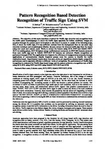
Evaluation with Real Datasets. We first evaluate the performance of all five competitors on the GMTI data, which is a representative for moving object monitoring applications. We use the query parameters learned from the pre-analysis of the data, including window size Q.win, θrange and θcount . We varied the slide size from 10% to 100% of Q.win. We find there are 6 to 11 clusters in the window at different time horizons, and N¯pi ranges from 9% to 11% of the number data points in the windows.
Figure 18: Comparison on CPU Time for Time-Based Window Scenario
as the experimental results show in Figures 18 and 19, Abstract-C clearly outperforms the naive solution and exact-STORM. Another experiment for the count-based window scenario shows that exact-STORM and Abstract-C perform equivalently well in terms of CPU time in most of the test cases. Details of these experiments as well as an analytical comparison between exact-STORM and Abstract-C can be found in [24].
8.
Figure 16: Comparison on CPU Time with GMTI data
Figure 17: Comparison on Memory Usage with GMTI data
As depicted in Figures 16 and 17, Extra-N has the best time efficiency compared with all other methods. The memory usage of Extra-N is on average 16% higher than the naive solution in the five cases. It is a little bit higher than that of Abstract-M, which is 11% higher than the naive solution, but still very acceptable. For STT dataset, similar behaviors of each algorithm as above can be observed, while the number of clusters in the windows ranges from 17 to 26, and N¯pi in the windows ranges from 6% to 9% of the number of data points. The result charts omitted here can be found in [24]. Generally, our experiments on real data also confirm that our proposed algorithm Extra-N and Abstract-M outperform other alternative methods and thus are the best solutions for density-based cluster detection in sliding windows.
7.4 Evaluation of Distance-Based Outlier Detection Methods To evaluate the performance of our outlier algorithm Abstract-C, we compare it with two alternatives, namely the naive solution and the exact-STORM presented by [3], which is the only previous work we are aware of that detects distance-based outliers in sliding windows. In our experiments, we compare the performance of exact-STORM and Abstract-C in both count- and time-based window scenarios. In both scenarios, we strictly followed the implementation of exact-STORM presented in [3], except for breaking the upper bound on the number of neighbors stored, as required in
Figure 19: Comparison on Memory Usage for TimeBased Window Scenario
RELATED WORK
Traditionally, pattern detection techniques are designed for static environments with large volumes of stored data. Well-known algorithms for static data clustering include [25, 18, 15, 4], and for detecting outliers include [22, 9, 20]. In these works, both clusters and outliers can either be global patterns [25, 18] that are defined by global characteristics of all data or local patterns [22, 4] that are defined by the characteristics of a subset of the data. In this work, our target pattern types are density-based clusters [15] and distance-based outliers [20]. Both are popular pattern types defined by local neighborhood properties. The early clustering algorithms applied to data streams [17, 16] are global clustering algorithms adapted from the static k-means algorithm. They treat the data stream clustering problem as a continuous version of static data clustering. They treat objects with different time horizons (recentness) equally and thus only reflect the accumulative features in data streams. [2] presented a framework of clustering streaming data using a two stage process. First, the online component summarizes streaming data into micro-clusters, each represented by a CFV (a statistical description of clusters). Then, an offline component clusters the micro-clusters formed earlier to form final clustering results using a static k-means algorithm. In this framework, a subtraction function is used to approximately discount the effect of the earlier data on the clustering results. Several extensions have been made to this work, focusing respectively on clustering multiple data streams [12] and parallel data streams [8]. None of efforts described above deals with arbitrarily shaped local clusters, nor do they support sliding window semantics. The only exception is [7] which discusses the clustering problem with sliding windows. However, it again is a global clustering algorithm maintaining approximated cluster centers only. Incremental DBSCAN [14] incrementally updates density-based clusters in data warehouse environments. However, as elaborated in our introduction and Section 5, this work does not solve the problem of efficiently discounting the effect of object “deleted" from the dataset. For this reason as well as because all optimizations in this work were designed for single updates (a single deletion or inser-
tion) to the data warehouse, it may fit well for the relatively stable environments but is not scalable to streaming environments that are highly dynamic. [11, 10] also studied the problem of detecting density-based clusters over streaming data. However, [11, 10] are not applied to identify the individual members in the clusters as required by the application scenarios described in the introduction. Also, to capture the dynamicity of the evolving data, they both use decaying factors derived from the “age" information of the objects. These decaying factors put lighter weights on older objects during the clustering processes. This approach emphasizes the recent stream portion more compared to the older data, but it does not enforce the discounting of old data’s effect from the pattern detection results. Thus, they cannot be used in the applications associated with sliding windows discussed in this work. Outlier Detection over data streams has been studied by [1, 23, 3]. Among these works, [1] works with outliers defined differently than ours. Thus, this technique cannot be applied to detect the distance-based outliers discussed in this work. [23] studes the detection of distance- and MEDF-based outliers in hierarchical structured sensor networks. The outliers detection is based on approximated data distribution, which is different from our approach of using exact objects. Most similar to our effort, the exact-STORM algorithm [3] also detects exact distance-based outliers within sliding windows. However, this work only deals with count-based windows, where the number of objects in the window is aprioir known and fixed. Our analytical and experimental studies reveal that this method is not suitable for handling time-based windows, where the numbers of objects in each window are different. Our work instead is more general yet efficient in both cases.
9. CONCLUSIONS In this work, we study the problem of incrementally detecting neighborbased patterns for sliding windows over streaming data. We first identify that the major difficulty of incremental detection of the neighbor-based patterns exists in the handling of expired objects. For this reason, our two primitive incremental algorithms Exact-N and Abstract-C suffer from either massive CPU or memory consumption for detecting density-based clusters. Then, we design the third algorithm Abstract-M based on a proposed “view prediction" technique, which elegantly discounts the effect of expired data points from the patterns. Finally, the combination of the “view prediction" technique and a proposed hybrid neighborship maintenance mechanism leads to an ideal solution Extra-N, achieving both linear memory consumption and the minimum number of range query searches. Both our analytical and experimental studies confirm that: 1) Our proposed algorithms Extra-N and Abstract-M are near-optimal in detecting density-based clusters over sliding windows in terms of CPU time, memory space and also scalability. 2) Our proposed algorithm Abstract-C is a CPU- and memoryefficient algorithm for distance-based outlier detection in sliding windows. It clearly outperforms the only previous algorithm [3] when detecting outliers in time-based windows, while performing equivalently with it when dealing with count-based windows.
10. REFERENCES [1] C. C. Aggarwal. On abnormality detection in spuriously populated data streams. In SDM, 2005. [2] C. C. Aggarwal, J. Han, J. Wang, and P. S. Yu. A framework for clustering evolving data streams. In VLDB, pages 81–92, 2003. [3] F. Angiulli and F. Fassetti. Detecting distance-based outliers in streams of data. In CIKM, pages 811–820, 2007.
[4] M. Ankerst, M. M. Breunig, H.-P. Kriegel, and J. Sander. Optics: Ordering points to identify the clustering structure. In SIGMOD. [5] A. Arasu, S. Babu, and J. Widom. The cql continuous query language: semantic foundations and query execution. VLDB J., 15(2):121–142, 2006. [6] A. Arasu and J. Widom. Resource sharing in continuous sliding-window aggregates. In VLDB, pages 336–347, 2004. [7] B. Babcock, M. Datar, R. Motwani, and L. O’Callaghan. Maintaining variance and k-medians over data stream windows. In PODS, pages 234–243, 2003. [8] J. Beringer and E. Hüllermeier. Online clustering of parallel data streams. Data Knowl. Eng., 58(2):180–204, 2006. [9] M. M. Breunig, H.-P. Kriegel, R. T. Ng, and J. Sander. Lof: identifying density-based local outliers. SIGMOD Rec., 29(2):93–104, 2000. [10] F. Cao, M. Ester, W. Qian, and A. Zhou. Density-based clustering over an evolving data stream with noise. In SDM, 2006. [11] Y. Chen and L. Tu. Density-based clustering for real-time stream data. In KDD, pages 133–142, 2007. [12] B.-R. Dai, J.-W. Huang, M.-Y. Yeh, and M.-S. Chen. Adaptive clustering for multiple evolving streams. IEEE Trans. Knowl. Data Eng., 18(9):1166–1180, 2006. [13] J. N. Entzminger, C. A. Fowler, and W. J. Kenneally. Jointstars and gmti: Past, present and future. IEEE Transactions on Aerospace and Electronic Systems, 35(2):748–762, april 1999. [14] M. Ester, H.-P. Kriegel, J. Sander, M. Wimmer, and X. Xu. Incremental clustering for mining in a data warehousing environment. In A. Gupta, O. Shmueli, and J. Widom, editors, VLDB, pages 323–333, 1998. [15] M. Ester, H.-P. Kriegel, J. Sander, and X. Xu. A density-based algorithm for discovering clusters in large spatial databases with noise. In KDD, pages 226–231, 1996. [16] S. Guha, A. Meyerson, N. Mishra, R. Motwani, and L. O’Callaghan. Clustering data streams: Theory and practice. IEEE Trans. Knowl. Data Eng., 15(3):515–528, 2003. [17] S. Guha, N. Mishra, R. Motwani, and L. O’Callaghan. Clustering data streams. In FOCS, pages 359–366, 2000. [18] J. A. Hartigan and M. A. Wong. A k-means clustering algorithm. Applied Statistics, 28(1). [19] I. INETATS. Stock trade traces. http://www.inetats.com/. [20] E. M. Knorr and R. T. Ng. Algorithms for mining distance-based outliers in large datasets. In VLDB, pages 392–403, 1998. [21] J. Munkres. Topology. Prentice Hall, 2000. [22] I. Ruts and P. J. Rousseeuw. Computing depth contours of bivariate point clouds. Comput. Stat. Data Anal., 23(1):153–168, 1996. [23] S. Subramaniam, T. Palpanas, D. Papadopoulos, V. Kalogeraki, and D. Gunopulos. Online outlier detection in sensor data using non-parametric models. In VLDB, pages 187–198, 2006. [24] D. Yang. Neighbor-based pattern detection for windows over streaming data. WPI Technical Report, 2008. http : //users.wpi.edu/ ∼ diyang/str_patt_detect.pdf . [25] T. Zhang, R. Ramakrishnan, and M. Livny. Birch: an efficient data clustering method for very large databases. SIGMOD Record, vol.25(2), p. 103-14, 1996.