damage and hydraulic loss over Baghdad [21], and the Sioux City, Iowa accident involving United Airlines Flight 232. [22]. The dissimilar actuator rates can ...
Neural Net Adaptive Flight Control Stability, Verification and Validation Challenges, and Future Research Nhan T. Nguyen Stephen A. Jacklin NASA Ames Research Center, Moffett Field, CA 94035 This paper provides a discussion of challenges of neural net adaptive flight control and an examination of stability and convergence issues of adaptive control algorithms. Understanding stability and convergence issues with adaptive control is important in order to advance adaptive control to a higher technology readiness level. The stability and convergence of neural net learning law are investigated. The effect of unmodeled dynamics on learning law is examined. Potential improvements in the learning law and adaptive control architecture based on optimal estimation are presented. The paper provides a brief summary of the future research of the Integrated Resilient Aircraft Control (IRAC) in the area of adaptive flight control. The paper also discusses challenges and future research in verification and validation.
1 Introduction While air travel remains the safest mode of transportation, accidents do occur on rare occasions with catastrophic consequences. For this reason, the Aviation Safety Program under the Aeronautics Research Mission Directorate (ARMD) at NASA has created the Integrated Resilient Aircraft Control (IRAC) research project to to advance the state of aircraft flight control and to provide onboard control resilience for ensuring safe flight in the presence of adverse conditions such as faults, damage, and/or upsets [1]. These hazardous flight conditions can impose heavy demands on aircraft flight control systems in their abilities to enable a pilot to stabilize and navigate an aircraft safely. The flight control research to be developed by the IRAC project will involve many different disciplines including aerodynamics, aircraft flight dynamics, engine dynamics, airframe structural dynamics, and others. During off-nominal flight conditions, all these conditions can couple together to potentially overwhelm a pilot’s ability to control an aircraft. The IRAC research goal is to develop vehicle-centric multidisciplinary adaptive flight control approaches that can effectively deal with these coupled effects. Modern aircraft are equipped with flight control systems that have been rigorously field-tested and certified by the Federal Aviation Administration. Functionally, an aircraft flight control system may be decomposed into an inner-loop and an outer-loop hierarchy. The outer-loop flight control is responsible for the aircraft guidance and navigation. It generates flight path or trajectory of the aircraft position based on pilot’s inputs to the Flight Management System (FMS). The FMS provides pilots with capabilities for performing pre-flight planning, navigation, guidance, and performance management using built-in trajectory optimization tools for achieving operational efficiencies or mission objectives. The inner-loop flight control has a dual responsibility in tracking the trajectory commands generated by the outer-loop flight control and, more importantly, in stabilizing the aircraft attitude in the pitch, roll, and yaw axes. Because the aircraft must be stabilized rapidly in an off-nominal event such as upsets or damage, the inner-loop flight control must have a faster response time than the outer-loop flight control. In a damage scenario, some part of a lifting surface may become separated and, as a result, may cause an aircraft’s center of gravity (C.G.) to shift unexpectedly. Furthermore, changes in aerodynamic characteristics can render a damaged aircraft unstable. Consequently, these effects can lead to a non-equilibrium flight that can adversely affect the ability of a flight control system to maintain aircraft stability. In other instances, reduced structural rigidity of a damaged airframe may manifest in elastic motions that can interfere with a flight control system, and potentially can result in excessive structural loading on critical lifting surfaces. Thus, in a highly dynamic, off-nominal flight environment with many sources of uncertainty, a flight control system must be able to cope with complex and uncertain aircraft dynamics.
1
The goal of the IRAC project is to arrive at a set of validated multidisciplinary integrated aircraft control design tools and techniques for enabling safe flight in the presence of adverse conditions [1]. Aircraft stability and maneuverability in off-nominal flight conditions are critical to aircraft survivability. Adaptive flight control is identified as a technology that can improve aircraft stability and maneuverability. Stability of adaptive control remains a major challenge that prevents adaptive control from being implemented in human-rated or mission-critical flight vehicles. Understanding stability issues with adaptive control, hence, will be important in order to advance adaptive control technologies. Thus, one of the objectives of IRAC adaptive control research is to develop metrics for assessing stability of adaptive flight control by extending the robust control concept of phase and gain margins to adaptive control. Furthermore, stability of adaptive control and the learning algorithms will be examined the presence of unmodeled dynamics and exogenous disturbances. Another objective of the IRAC research is to advance adaptive control technologies that can better manage constraints placed on the aircraft. These constraints are dictated by limitations of actuator dynamics, aircraft structural load limits, frequency bandwidth, system latency, and others. New concepts of adaptive control will be developed to address these constraints.
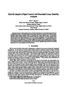
2 Convergence and Stability of Neural Net Direct Adaptive Flight Control Over the past several years, various adaptive control techniques have been investigated [4, 5, 7, 8, 9, 10, 13, 15, 11]. Adaptive flight control provides a possibility for maintaining aircraft stability and performance by means of enabling a flight control system to adapt to system uncertainties. Meanwhile, a large area of research in intelligent control has emerged and spans many different applications such as spacecraft and aircraft flight control. An essential element of an intelligent flight control is a neural network system designed to accommodate changes in aircraft dynamics due to system uncertainties. Neural network is known to be a good universal approximator of many nonlinear functions that can be used to model system uncertainties. In the implementation of an intelligent flight control, the neural network is usually incorporated within a direct adaptive control architecture to provide an augmentation to a pilot command. The neural network estimates the system uncertainties and outputs directly a command augmentation signal that compensates for changes in aircraft dynamics. Research in adaptive control has spanned several decades, but stability robustness in the presence of unmodeled dynamics, parameter uncertainties, or disturbances as well as the issues with verification and validation of adaptive flight control software still pose as major challenges[5, 2]. Adaptive control laws may be divided into direct and indirect approaches. Indirect adaptive control methods typically compute control parameters from on-line learning neural networks that perform plant parameter estimation [6]. Parameter identification techniques such as recursive least-squares and neural networks have been used in indirect adaptive control methods [7]. In recent years, modelreference direct adaptive control using neural networks has been a topic of great research interest [8, 9, 10]. Lyapunov stability theory has been used to test theoretical stability of neural network learning laws. NASA has been developing an intelligent flight control technology based on the work by Rysdyk and Calise [8]. An architecture of the intelligent flight control is as shown in Fig. 1.
Fig. 1 - Neural Net Adaptive Flight Control Architecture Recently, this technology has been demonstrated on an F-15 fighter aircraft [12]. The intelligent flight control uses a model-reference, direct adaptive, dynamic inversion control approach. The neural network direct adaption is designed to provide consistent handling qualities without requiring extensive gain-scheduling or explicit system 2
identification. This particular architecture uses both pre-trained and on-line learning neural networks and a reference model to specify desired handling qualities. Pre-trained neural networks are used to provide estimates of aerodynamic stability and control characteristics. On-line learning neural networks are used to compensate for errors and adapt to changes in aircraft dynamics. As a result, consistent handling qualities may be achieved across flight conditions. Recent flight test results demonstrate the potential benefits of adaptive control technology in improving aircraft flight control systems in the presence of adverse flight conditions due to failures [19]. The flight test results also point out the needs for further research to increase the understanding of effectiveness and limitations of the direct adaptive flight control. One potential problem with the neural net direct adaptive flight control is that high gain control used to facililate aggressive learning to reduce the error signal rapidly can potentially result in a control augmentation command that may saturate the control authority or excite unmodeled dynamics of the plant that can adversely affect the stability of the direct adaptive learning law.
2.1 Direct Adaptive Control Approach Adaptive flight control is designed to accommodate parametric and system uncertainties in the presence of adverse conditions such as upset, failures, and damage. The true aircraft dynamics may be described by a linear model about its trim point in a flight envelope ω˙ = ω˙ ∗ + ∆ω˙ = F1 ω + F2 σ + Gδ (1) � �> � �> is the aircraft angular rate, σ = ∆α ∆β ∆φ is an incremental trim state vector to where ω = p q r maintain trim condition, ∆ω˙ is the unknown aircraft dynamics due to parametric uncertainties, and ω˙ ∗ is the nominal aircraft dynamics described by ω˙ ∗ = F∗1 ω + F∗2 σ + G∗ δ (2) where F∗1 , F∗2 , and G∗ as the nominal plant matrices which are assumed to be known. The input to the dynamic inversion controller is a desired acceleration command
ω˙ d = F∗1 ω + F∗2σ + G∗δ
(3)
The difference in the aircraft dynamics gives rise to the modeling error ε which is defined as
ε = ω˙ − ω˙ d = ∆F1 ω + ∆F2σ + ∆Gδ
(4)
The modeling error that exists in the controller causes the aircraft states to deviate from its desired states. This results in a tracking error dynamics which are described by e˙ = Ae + B (uad − ε )
(5)
�> � Rt is a proportional-integral tracking error with ω e = ω m − ω defined as the rate error where e = 0 ω edτ ω e signal which is the difference between a reference model rate ω m and the actual aircraft rate, uad is the neural net direct adaptive signal, and A and B are matrices defined as � � � � 0 0 I , B= A= (6) I −KI −KP The reference model rate ω m is described by a first order model that gives the flight controller a suitable handling characteristic. To compensate for the parametric uncertainties, the neural net direct adaptive signal uad uses a linearin-parameter sigma-pi network proposed by Rysdyk and Calise [8]. This network is further modified [18] to include additional inputs as shown in Fig. 2.
3
Fig. 2 - Sigma-Pi Neural Network Associated with the neural network is a set of weights that are adjusted on-line in order to enable the flight control system to adapt to changes in aircraft dynamics. The neural net direct adaptive signal and the weights are computed by uad = W> β (7)
� �
˙ = −Γ β e> PB + µ W (8)
e> PB W where Γ is the learning rate, µ is the e-modification term, β is a basis function comprising neural net inputs Ci , i = 1, . . . , 6, and P is the solution of the Lyapunov equation A> P + P>A = −Q
(9)
where Q is a positive-definite matrix.
2.2 Stability and Convergence A key challenge with neural net adaptive flight control is to make the learning algorithm sufficiently robust. Robustness relates to the stability and convergence of the learning algorithm. Stability is a fundamental requirement of any dynamical system that ensures a small disturbance would not grow to a large deviation from an equilibrium. For systems with high assurance such as human-rated or mission-critical flight vehicles, stability of adaptive systems is of paramount importance. Without guaranteed stability, such adaptive control algorithms cannot be certified for operation in high-assurance systems. Unfortunately, the stability of adaptive controllers in general and neural net adaptive controllers in particular remains unresolved. The notion of a self-modifying flight control law using an artificial neural net learning process whose outputs may be deemed as non-deterministic is a major huddle to overcome. Another criterion for robustness is the convergence of the neural net learning algorithm. Neural networks are used as universal nonlinear function approximators. In the case of the adaptive flight control, the networks approximate the unknown modeling error that is used to adjust effectively the control gains to maintain a desired handling quality. Convergence requires stability and a proper design of the weight update law. It is conceivable that even though a learning algorithm is stable, the neural net weights may not converge to correct values. Thus, accurate convergence is also important since this is directly related to the flight control performance. Referring to Eq. (5), if the direct adaptive signal uad could perfectly cancel out the modeling error ε , then the tracking error would tend to zero asymptotically. Therefore, ideally the desired acceleration ω˙ d would perfectly track the reference model acceleration ω˙ m . In practice, there is always some residual modeling error in the adaptation, so asymptotic stability of the tracking error is not guaranteed. Instead, a weaker uniform stability of the tracking error can be established by the Lyapunov stability theory. The tracking error dynamics is then bounded from below by ˜ > β + ∆e e˙ ≤ Ae + BW ˜ is the neural net weight matrix variation and ∆e is the approximation error defined as where W
�
�
∆e = sup B W∗> β − ε ≤ sup W∗> β − ε β
β
4
(10)
(11)
where W∗ is the ideal weight matrix which is equal to ˜ W∗ = W − W
(12)
It can be shown by the Lyapunov analysis [18] that there exists a δ -neighborhood that the tracking error is attractive to and remains bounded from below � ρ (P) � δ = inf kek = (13) 4 k∆e k + µ kW∗ k2 ω 2ρ (Q)
where ρ denotes the spectral radius of a matrix. Thus, if δ is sufficiently small, then the tracking error will be reasonably close to zero. This means that the neural net approximation error is also small and the tracking performance is good. The neural net weight update law in Eq. (8) is nonlinear due to the product term of the basis function β and the tracking error e. Stability of nonlinear systems is usually analyzed by the Lyapunov method. However, the concept of phase and gain margin for linear systems cannot be extended to nonlinear adaptive control. The linear control margin concept can provide understanding stability margin of adaptive control that enables a more robust adaptive learning law to be synthesized. This is only possible if the neural net weight update law is linearized at a certain point in time with the neural net weights held constant. As adaptation occurs, the neural net weights vary with time. Hence, the time at which to freeze the neural net weights (for calculation) must correspond to a worst-case stability margin. This can be a challenge. Therefore, this paper introduces a new method for analyzing stability and convergence of the nonlinear neural net weight update law using error bound analysis, which enables the dominant linear component of the nonlinear neural net weight update law to be extracted from Eq. (8) without linearizing the adaptive control law at an instance in time. Towards that end, we note that Eq. (8) can be expressed as
� � d � > � >
β W = −Γ β > β e> PB + µ e> PB β > W + β˙ W dt
We define an error bound on the neural net adaptive signal as
˜>˙
∆W˜ = sup W β − Γµ e> PB W∗> β β
(14)
(15)
Then, the time derivative of the variation in the neural net adaptive signal is bounded by
� � d �˜> �
˜> W β ≤ −Γ α B> Pe + µ e> PB W β + ∆W˜ dt
(16)
where α > 0 is defined as a level of persistent excitation (PE) such that the following PE condition is satisfied Z
> 1 t+T > β β dτ ≤ α
β β = T t
(17)
for β ∈ L2 . Thus, without sufficient persistent excitation and if the e-modification parameteter µ is not present, the neural net weights will not necessarily converge. The persistent excitation essentially means that inputs to the neural network must be sufficiently rich in order to excite system dynamics to enable a convergence to take place. If the error bound is small, then the linear behavior of the weight update law becomes dominant. Therefore, this enables the stability and convergence to be analyzed in a linear sense using the following equation � � � � � �� � d A B e e ∆e
≤ + (18) ˜ >β ˜ >β ∆W˜ −Γα B> P −Γµ e> PB W dt W
The stability of the learning law thus requires the leading matrix to be negative definite. This can be established by computing its eigenvalues from the following characteristic equation
� �
(A − Λ) −Γµ e> PB I − Λ + Γα BB> P = 0 (19) 5
This is a matrix quadratic equation whose solution can only be computed numerically since a general quadratic matrix equation x2 + bx + c = 0 (20) where x, b, c ∈ [Cn × Cn ] does not have the following solution b x=− ± 2
#1 "� � 2 b 2 −c 2
(21)
where the square root is a matrix operator that operates on the eigenvalues of the radicand. However, if b and c are commutative, then Eq. (21) is the solution [24]. One notes that Eq. (19) is bounded from above by
�
�
Λ2 − A − Γµ e> PB I Λ − Γµ e> PB A + Γα BB> P I = 0 (22)
which satisfies the commutative property. Therefore, the solution of this characteristic matrix equation is equal to #1 "
�2
2 A − Γµ e> PB I A − Γµ e> PB I
>
> ± + Γµ e PB A − Γα BB P I Λ= 2 4
(23)
There exists a constant γ > 0 such that the learning rate is bounded by
�2
γ A + Γµ eT PB I ≤ε Γ −
4α BB> P
(24)
Then it follows that
A − Γµ e> PB I A + Γµ e> PB I p ± 1−γ Λ≤ 2 2 If Λ is negative definite, then the rate of convergence is established by the eigenvalues of Λ since �
e ˜ >β W
�
Λt
≤ Φe Φ
−1
�
e (0) ˜ (0)> β (0) W
�
−
�
A
B
−Γα B> P −Γµ e> PB
�−1 �
where Φ is a matrix of right eigenvectors of the leading matrix. The equilibrium is therefore uniformly asymptotically stable and converges to
� � �−1 �
e A B ∆
e
= lim sup
˜ > β −Γα B> P −Γµ e> PB ∆W˜ t→∞ β W By Holder’s inequality, the convergence radius can be expressed as
e � −1 ∆e
lim sup ˜ > ≤ ρ Λ
∆˜ t→∞ β W β W
∆e ∆W˜
(25)
�
(26)
(27)
(28)
Thus, ∆e and ∆W˜ should be kept as small as possible for the tracking error and the neural net weight matrix variation to converge as close to zero as possible. In order to obtain a convergence, stability of the tracking error and neural net weight update law must be established by the negative-definiteness of the eigenvalues of Λ. Consider the following cases: 1. γ � 1:
This √ corresponds to a small learning rate or slow adaptation. Using the first two terms of the Taylor series of 1 − γ and retaining linear terms of Γ, we have � � � γ� λ (Λ1 ) ≈ 1 − λ (A) ≈ λ A − Γα A−1BB> P (29) 4 6
γ γ
λ (Λ2 ) ≤ −Γµ e> PB + λmax (A) = 4 4
where λ is the eigenvalue operator of a matrix.
! µ e> PB A2
λmax (A) − α BB> P
(30)
The eigenvalues of Λ2 correspond to the neural net weight update law which indicates that the neural net learning is very slow. The eigenvalues of Λ1 correspond to the tracking error dynamics. Since KP > 0 and KI > 0, then A is Hurwitz, i.e., A possesses negative eigenvalues. Thus, the tracking error dynamics are stable and the eigenvalues of Λ1 are � 21 � � � 2 γ K KP λ (Λ1 ) ≈ 1 − λ − ± j KI − P (31) 4 2 4 whereupon, to achieve good loop gains, the integral gain should be set such that the negative real part of the maximum eigenvalue is greatest or K2 (32) KI ≥ P 4 The convergence radius is then approximately equal to
e
∆e 4
lim sup ˜ > ≤ (33) ∆W˜ t→∞ β W β µ e> PBkkA2 k k γ λmax (A) − α BB> P k k
Since γ is small, the convergence radius is large and thus the neural network would not achieve a good convergence. It should be noted that a large value of µ has the same effect as slow adaptation since this corresponds to a small value of γ . Thus, while µ tends to provide robustness to the adaptive control algorithm, it also slows down the speed of learning of the neural network, thereby leading to poor convergence. 2. γ � 1:
This corresponds to a large learning rate or fast adaptation only when µ = 0. When the learning rate is large and µ 6= 0, the effect is equivalent to that with small γ as discussed previously. For µ = 0, the eigenvalues of the tracking error dynamics and neural net weight update law then become more complex-valued � � √ A λ (Λ) ≈ λ (34) (1 ± j γ ) 2 The convergence radius is then approximately equal to
e
∆e 2
lim sup ≤ >
˜ t→∞ β W β (1 + γ )|λmax (A)| ∆W˜
(35)
Since γ is large, the convergence radius is small and thus the neural network would have a good convergence.
If µ 6= 0, then in the limit for a very large learning rate, the neural net weights in theory would converge to > ˜ > β = − α B Pe lim W Γ→∞ µ e> PB
(36)
and the tracking error dynamics would become e˙ ≤
α BB> P
A− µ e> PB
!
e + ∆e
(37)
Thus, in theory, a large learning rate would improve stability and convergence. However, in practice there exists a potential problem with a large learning rate. Equation (34) shows that increasing the learning rate to a large value with µ = 0 will result in a high frequency oscillation in the adaptive signal [20]. This high frequency 7
oscillation can result in excitation of unmodeled dynamics that may be present in the system and therefore can lead to a possibility of instability since the effects of unmodeled dynamics are not accounted in the Lyapunov analysis of the neural net weight update law [6]. When µ 6= 0, increasing the learning rate does not lead to a high frequency oscillation which tends to improve robustness, but the convergence is poorer. Thus, high-gain learning should be avoided in adaptive control. Another source of instability is measurement noise which will also influence high-gain controllers to make over-corrections. Stated loosely, the neural network then maps the spurious noise signals to small changes in the control commands, leading to a loss of true learning and instability. For this reason, learning is typically disabled when the error falls below a certain value by applying a dead band. To illustrate the effects of learning rate, a simulation was performed for a damaged twin-engine generic transport model (GTM) [3], as shown in Fig. 3. A wing damage simulation was performed with 25% of the left wing missing. The neural net direct adaptive control is implemented to maintain tracking performance of the damaged aircraft. A pitch doublet maneuver is commanded while the roll and yaw rates are regulated near zero.
Fig. 3 - Generic Transport Model Figure 4 illustrates the effect of learning rate without the e-modification term, i.e, µ = 0. Without adaptation, the performance of the flight control is very poor as significant overshoots occur. With adaptation, good tracking performance can be obtained. As the learning rate increases, the tracking error becomes smaller but high frequency signals also appear that is consistent with the analysis above. 0.05
q, rad/sec
q, rad/sec
0.05
0
0
2
Γ=10
Γ=0 −0.05 0
10
20 t, sec
30
−0.05 0
40
20 t, sec
q, rad/sec
0
40
0
Γ=103 −0.05
30
0.05
0.05
q, rad/sec
10
0
10
20
30
Γ=104 40
−0.05 0
10
t, sec
20 t, sec
30
40
Fig. 4 - Pitch Rate (µ = 0) Figure 5 is a plot of selected neural net weights for various learning rates. As can be seen, large learning rate causes high frequency oscillations in the weights. The convergence of the neural net weights Wq,q and Wq,δe associated with linear elements q and δe for the pitch rate are poor. Neither of these weights would actually converge to their correct values. Thus, convergence accuracy is not demonstrated. 8
−4
0.06
15
x 10
2
Γ=10 3 Γ=10 4 Γ=10
10 q,r
q,q
0.04
5
W
W
0.02
2
0 −0.02 0
Γ=10 3 Γ=10 Γ=104
0 10
20
30
−5 0
40
10
20
30
40
−3
0.2
3
x 10
2
2
t, sec r
2
Γ=10 3 Γ=10 4 Γ=10
W
e
0
q,δ
W
t, sec
r,δ
0.1
Γ=10 3 Γ=10 4 Γ=10
−0.1
1
−0.2 −0.3 0
10
20
30
0 0
40
10
20 t, sec
30
40
Fig. 5 - Neural Net Weight Learning (µ = 0) 0.05
q, rad/sec
q, rad/sec
0.05
0
0
µ=0.1
µ=0 −0.05 0
10
20 t, sec
30
−0.05 0
40
20 t, sec
30
10
20 t, sec
30
40
0.05
q, rad/sec
q, rad/sec
0.05
10
0
0
µ=1 −0.05 0
10
20 t, sec
30
µ=10 40
−0.05 0
40
Fig. 6 - Pitch Rate with µ 6= 0 (Γ = 1000) −4
0.005
10
−0.005 10
20 t, sec
0.2
µ=0 µ=0.1 µ=1 µ=10
5
−5 0
40
3
30
40
r,δr
1 0 −1 0
30
µ=0 µ=0.1 µ=1 µ=10
2
−0.2 0
20 t, sec
20 t, sec
x 10
−0.1 10
10 −3
W
e
q,δ
0
x 10
0
µ=0 µ=0.1 µ=1 µ=10
0.1 W
30
W
µ=0 µ=0.1 µ=1 µ=10
0
−0.01 0
q,r
15
Wq,q
0.01
40
10
20 t, sec
30
40
Fig. 7 - Neural Net Weight Learning (Γ = 1000) Figure 6 illustrates the effect of the e-modification parameter µ . As µ increases, the high-frequency amplitude reduces but the tracking error becomes worse. Eventually, with large enough value of µ , the learning essentially ceases. Figure 7 is the plot of selected neural net weights. Clearly, with increasing µ , the weights are driven to zero, thereby reducing the learning of the neural network. This is consistent with the analysis above which shows the for learning rate with µ 6= 0, the effect is essentially the same as that with small learning rate. 9
2.3 Unmodeled Dynamics Unmodeled dynamics are secondary dynamics that are ignored in the system dynamics. Usually, the small effects of unmodeled dynamics can be quite important, but sometimes are not explicitly accounted for in a control design due to the complexity of the physical modeling. An example of secondary dynamics is the structural dynamics of the airframe undergoing elastic deformation in flight. Typically, if the controller possesses sufficient gain and phase margins, then the controller can be verified during validation to ensure that it is sufficiently robust to safeguard against potentially destabilizing effects of unmodeled dynamics. Unmodeled dynamics can have a profound effect on the stability of the learning algorithms for adaptive control. Even though an adaptive control algorithm may demonstrate stability for a dominant system dynamics, it can become unstable when a small unmodeled dynamics is present in the system. This can be shown by considering the following aircraft dynamics ω˙ = F1 ω + F2 σ + Gδ − z (38) where z is a small parasitic state that represents the effects of unmodeled dynamics that have a certain property which can be described by ε z˙ = −z − η Gδ (39)
where ε > 0 and η > 0 are small parameters. Additionally, let the measurement output of the aircraft be the angular rate vector y=ω (40) Then, the unmodeled dynamics are expressed as � � ˜ > β + ε ∆z ε z˙ ≤ −z − η GG∗−1 B> Ae + W
where
η GG∗−1 W∗> β − ω˙ � m
∆z = sup
ε β
(41)
(42)
The unmodeled dynamics affect the tracking error dynamics according to ˜ > β + Bz + ∆e e˙ ≤ Ae + BW
The dynamics of the combined system are bounded by A B B e e ∆e
d ˜> ˜ >β + ∆ ˜ −Γα B> P −Γµ e> PB 0 W ≤ W β W dt η η 1 ∗−1 > ∗−1 ∆z z z − ε GG −ε − ε GG B A
We consider the case when µ = 0. The characteristic equation is obtained as � � � � � η I A Γα B 3 2 ∗−1 > > I − η GG∗−1 B> P = 0 s + −A s + BGG B A − + Γα BB P s + ε ε ε ε
(43)
(44)
(45)
Applying the Routh-Hurwitz criterion, the following matrix inequalities are required for stability of the system I −A > 0 ε
(46)
� � η A Γα B ∗−1 > > I − η GG∗−1 B> P > 0 (47) BGG B A − + Γα BB P − ε ε ε � Γα B I − η GG∗−1 B> P > 0 (48) ε Inequality (46) is satisfied identically since A is Hurwitz. Inequality (48) is also satisfied since P is positive-definite and η is small. Inequality (47) requires the learning rate to satisfy the following inequality � � 1 Γα η BGG∗−1 B> P + ε ABB> P < D (49) ε �
I −A ε
��
10
where
� � D = (I − ε A) η BGG∗−1 B> A − A > 0
(50)
Thus, if the learning rate is sufficient large and the left hand side expression is positive-definite, it is conceivable that stability requirements could be violated, thereby resulting in instability of the adaptive control algorithm. Clearly, large learning rate can lead to a fast adaptation and large parasitic state z which acts as a disturbance to the dominant system dynamics, thereby leading to faulty adaptation that can result in unbounded solutions. For stability and bounded solutions, the learning rate should be kept small such that the speed of adaptation should be slow relative to the speed of the parasitic state [6]. However, small learning rate will result in less than desired command-tracking performance. Therefore, a suitable learning rate is one that strives to achieve a reasonable balance between stability and performance of an adaptive flight control. In essence, this means that the acceptable gains for a stable neural net learning law must be found by trial and error, yet guided by theory and known structures of unmodeled dynamics, if possible. Figure 8 illustrates the effects of unmodeled dynamics on the learning of the adaptive control. The unmodeled dynamics result in a poor response when adaptation is off, but once adaptation is switched on, improvements can be immediately obtained. Comparing with Fig. 4, the high learning rate excites the unmodeled dynamics, thereby causing an increase in the undesired high frequency noise in the adaptive signals. With sufficiently large learning rate, the weight update law would become unstable. 0.05
0.05
q, rad/sec
q, rad/sec
0.1
0
0
−0.05
2
Γ=10
Γ=0 −0.1 0
10
20 t, sec
30
−0.05 0
40
20 t, sec
30
40
0.05
q, rad/sec
q, rad/sec
0.05
10
0
0
4
3
Γ=10
Γ=10 −0.05 0
10
20 t, sec
30
40
−0.05 0
10
20 t, sec
30
40
Fig. 8 - Pitch Rate with Unmodeled Dynamics (µ = 0, ε = 0.1, η = 0.1)
3 Potential Improvements In the neural net weight update law in Eq. (8), the tracking error signal e is used for adaptation. This adaptive law is based on the stability analysis of the tracking error using the Lyapunov method [8]. Examining Eq. (5), one sees that if the adaptive signal uad could cancel out the modeling error ε , then the tracking error will tend to zero asymptotically. Thus, if the modeling error ε is used for adaptation, potential improvements can be obtained. We now introduced two methods of alternate adaptive control in lieu of the existing method.
3.1 Direct Adaptive Control with Recursive Least Squares In this approach, we will design a neural net weight update law that minimizes the non-homogeneous term in Eq. (5). We will use the optimal estimation method to minimize the following cost functional J (W) = where
1 2
Z t 0
2
(1 + ξ )−1 W> β − εˆ d τ
εˆ = ε − ∆ε = ω˙ˆ − ω˙ d = ω˙ˆ − F∗1ω − F∗2σ − G∗δˆ ξ = β > Rβ 11
(51)
(52) (53)
∆ε is the estimation error of the modeling error ε since aircraft angular accelerations ω˙ may not be directly measured and thus requires to be estimated. ξ is viewed as a weighted PE condition that is required for improved convergence with R as a positive-definite weighting matrix. A larger R results in a faster convergence. R can also be viewed as a learning rate matrix. To minimize the cost functional, we compute its gradient with respect to the neural net weight matrix and set it to zero, thus resulting in Z t � � > (54) (1 + ξ )−1 β β > W − εˆ > d τ = 0 ∇JW = 0
Equation (54) is then written as
Z t 0
(1 + ξ )−1 β β > d τ W =
Let R−1 =
Z t 0
Z t 0
(1 + ξ )−1 β εˆ > d τ
(1 + ξ )−1 β β > d τ
(55)
(56)
We then note that ˙ −1 R + R−1R ˙ =0 R−1 R = I ⇒ R
(57)
˙ = −RR ˙ −1 R = − (1 + ξ )−1 Rβ β > R R
(58)
˙ + (1 + ξ )−1 β β > W = (1 + ξ )−1 β εˆ > R−1 W
(59)
˙ yields Solving for R Differentiating Eq. (55) yields
˙ yields the neural net weight update law Solving for W � � ˙ = − (1 + ξ )−1 Rβ β > W − εˆ > W
(60)
Equation (60) is a gradient-based recursive least-squares neural net weight update law that minimizes the neural net approximation error. In the process, the tracking error should decrease optimally to some minimum convergence radius. Comparing this neural net weight update law to that in Eq. (8), it is seen that the estimated modeling error εˆ is used for adaptation instead of tracking error. Moreover, the learning rate is also adaptive in that the weighting matrix R also needs to be updated by Eq. (58). The recursive least-squares neural net weight update law can be shown to be stable and result in bounded signals. ˜ with the asterisk and tilde symbols denoting ideal neural net weight matrix and neural To show this, let W = W∗ + W net weight matrix deviations, respectively. The following Lyapunov candidate function is chosen � � ˜ > R−1 W ˜ L = e> Pe + tr W (61) The time rate of change of the Lyapunov candidate function is computed as � � ˙˜ + W ˜ > R−1 W ˜ >R ˙ −1 W ˜ L˙ = e˙ > Pe + e> P˙e + tr 2W
(62)
With large enough R, the ideal neural net weight matrix W∗ can be shown to converge to the estimated modeling error εˆ [6] so that ˙˜ = − (1 + ξ )−1 Rβ β > W ˜ W (63) Upon simplification, one obtains � � ˜ >β β >W ˜ ≤0 L˙ = −e> Qe − (1 + ξ )−1 tr W
(64)
which requires a δ -neighborhood that the tracking error is attractive to and remains bounded from below
δ = inf kek =
2ρ (P) k∆ε k ρ (Q)
12
(65)
Since L˙ is negative semi-definite, the recursive least-squares method is uniformly asymptotically stable. Let R = ΓI, then the system dynamics of the recursive least-squares method are bounded by the following equation A B B e e ∆ε d ˜> −1 ˜ >β + ˜ ≤ (66) W β 0 − (1 + ξ ) Γα I 0 W W dt η η 1 ∗−1 > ∗−1 ∆z z z − ε GG −ε − ε GG B A
The characteristic equation of this system is obtained as
� � �� � �� I I η BGG∗−1 B> −1 −1 2 s + − A + (1 + ξ ) Γα I s + − I A + (1 + ξ ) Γα −A s ε ε ε � (1 + ξ )−1 Γα � η BGG∗−1 B> − I A = 0 + ε 3
�
(67)
Without the effects of unmodeled dynamics, this characteristic equation yields two roots, both of which are on the left half s-plane s1 = λ (A) (68) Γα (69) 1 + Γα Since s2 is a negative real root corresponding to the neural net weight matrix variation, increasing the learning rate would simply drive s2 farther to the left on the real axis of the s-plane. Therefore, unlike the current neural net direct adaptive control approach, large learning rate does not generate high frequency oscillations with the recursive least-squares method. Also, the rate of convergence tends to unity for large learning rate. Applying the Routh-Hurwitz criterion, the stability requirements due to the effects of unmodeled dynamics result in the following matrix inequalities I − A + (1 + ξ )−1 Γα I > 0 (70) ε s2 = − (1 + ξ )−1 Γα ≈ −
�
� � �� � �� I η BGG∗−1 B> I − A + (1 + ξ )−1 Γα I − I A + (1 + ξ )−1 Γα −A ε ε ε −
� (1 + ξ )−1 Γα � η BGG∗−1 B> − I A > 0 ε
(71)
� (1 + ξ )−1 Γα � η BGG∗−1 B> − I A > 0 (72) ε It can be shown that these inequalities are satisfied for A < 0, P > 0, and small ε and η . Therefore, the recursive least-squares method would tend to be less sensitive to unmodeled dynamics than the current neural net direct adaptive control. Figures 9, 10, and 11 illustrate the potential improvements due to the direct adaptive control with the recursive least-squares neural net weight update law. As can be seen from Fig. 9, the recursive least-squares learning provides a significant improvement in the tracking performance of the adaptive control. Moreover, increasing the learning rate does not cause high frequency oscillations as in the case of the current direct adaptive control approach. This is in agreement with the analysis which shows that the root s2 corresponding to the neural net weight update law does not have an imaginary part. Figure 10 is the plot of the selected neural net weights. The weights exhibit a nice convergence behavior. Increasing the learning rate causes the weight to move closer to the true values of the system parameters for which the adaptive control is compensating. In contrast, the neural net weights in the current adaptive control approach do not converge correctly to their true values, as shown in Fig. 5. Figure 11 shows the recursive least-squares learning in the presence of unmodeled dynamics. In contrast with the current method as shown in Fig. 8, the recursive least-squares learning is able to handle unmodeled dynamics much better. Increasing the learning rate does not cause increased high frequency oscillations. So the sensitivity to unmodeled dynamics is much less of an issue with the recursive least-squares learning. This behavior is in agreement with the analysis. 13
0.05
q, rad/sec
q, rad/sec
0.05
0
0
2
Γ=10
Γ=0 −0.05 0
10
20 t, sec
30
−0.05 0
40
20 t, sec
0
40
0
Γ=104
Γ=103 −0.05 0
30
0.05
q, rad/sec
q, rad/sec
0.05
10
10
20 t, sec
30
−0.05 0
40
10
20 t, sec
30
40
30
40
Fig. 9 - Pitch Rate with RLS Method 10
0.4 2
0.3 q,r
q,q
5 2
0
−5 0
10
20 t, sec
30
W
W
Γ=10 3 Γ=10 4 Γ=10 True Value
0.2
Γ=10 3 Γ=10 4 Γ=10 True Value
0.1 0 −0.1 0
40
1
10
20 t, sec
0.1 2
Γ=10 3 Γ=10 4 Γ=10 True Value
0.05
W
0
−0.5 0
10
20 t, sec
30
r,δr
2
Γ=10 3 Γ=10 4 Γ=10 True Value
W
q,δe
0.5
0 −0.05 −0.1 −0.15 0
40
10
20 t, sec
30
40
Fig. 10 - Neural Net Weight Learning with RLS Method 0.05
0.05
q, rad/sec
q, rad/sec
0.1
0
0
−0.05
Γ=102
Γ=0 −0.1 0
10
20 t, sec
30
−0.05 0
40
20 t, sec
0
40
0
Γ=103 −0.05 0
30
0.05
q, rad/sec
q, rad/sec
0.05
10
10
20 t, sec
30
Γ=104 40
−0.05 0
10
20 t, sec
30
40
Fig. 11 - Pitch Rate with RLS Method and Unmodeled Dynamics (ε = 0.1, η = 0.1)
3.2 Hybrid Direct-Indirect Adaptive Control with Recursive Least-Squares Another adaptive control architecture that has recently been proposed is hybrid adaptive control [18]. This architecture is as shown in Fig. 12. The hybrid adaptive control blends both direct and indirect adaptive control methods together 14
to provide a more effective control strategy. The indirect adaptive control is responsible for updating the dynamic inversion controller with a more accurate plant model which is estimated by the recursive least squares method. Any residual tracking error as a result of the dynamic inversion can then be handled by the neural net direct adaptive control.
Fig. 12 - Hybrid Adaptive Flight Control The dynamic inversion controller is updated by the estimated plant model at every time step according to ˆ −1 ω˙ d − Fˆ 1 ω − Fˆ 2 σ δ =G
�
(73)
ˆ = G ∗ + ∆G ˆ are the estimated plant matrices of the true plant model and G ˆ is where Fˆ 1 = F∗1 + ∆Fˆ 1 , Fˆ 2 = F∗2 + ∆Fˆ 2 , G assumed to be invertible. The hybrid adaptive control performs explicit parameter identification of the plant model to account for changes in aircraft dynamics. The parameter identification process is performed by the recursive least-squares method � � ˙ = − (1 + ξ )−1 Rθ θ > Φ − εˆ > Φ (74)
h � � > where Φ> = Wω Wσ> Wδ> is a neural net weight matrix and θ > = ω > β > ω matrix The estimated plant matrices are then updated as
σ >β > σ
δ >β > δ
i
is an input
T βω Fˆ 1 = F∗1 + Wω
(75)
Fˆ 2 = F∗2 + WTσ β σ
(76)
ˆ = G∗ + WT β G δ δ
(77)
The performance of the hybrid adaptive control is very similar to the recursive least-squares direct adaptive control with large values of R. At smaller values of R, the adaption is shared between the neural net direct and indirect adaptive control blocks. Thus, the learning rate of the neural net direct adaptive control can be turned down to reduce potential excitation of unmodeled dynamics as discussed earlier. The advantage of the hybrid adaptive control method is the ability to be able to estimate plant model parameters on-line. Direct adaptive control approaches accommodate changes in plant dynamics implicitly but do not provide an explicit means for ascertaining the knowledge of the plant dynamics. By estimating the plant model parameters explicitly using the recursive least-squares neural net learning law, an improved knowledge of the plant dynamics can be obtained that can potentially be used to develop fault detection and isolation (FDI) strategies, and emergency flight planning to provide guidance laws for energy management in the presence of hazards.
15
4 Verification and Validation Challenges for Adaptive Systems Creating certifiable adaptive flight control systems represents a major challenge to overcome. Adaptive control systems with learning algorithms will never become part of the future unless it can be proven that this software is highly safe and reliable. Rigorous methods for adaptive software verification and validation must therefore be developed by NASA and others to ensure that control system software failures will not occur, to verify that the control system functions as required, to eliminate unintended functionality, and to demonstrate that FAA certification requirements can be satisfied. The ability of an adaptive control system to modify a pre-designed flight control system is at the same time a strength and a weakness. On the one hand, the premise of being able to accommodate vehicle degradation is a major selling point of adaptive control since traditional gain-scheduled control methods are viewed to be less capable of handling off-nominal flight conditions outside their design operating points. Nonetheless, gain-scheduled control approaches are robust to disturbances and secondary dynamics. On the other hand, as previously shown in this paper, potential problems with adaptive control exist with regards to high-gain learning and unmodeled dynamics. Clearly, adaptive control algorithms are sensitive to these potential problems as well as others that have not been considered such as actuator dynamics, exogenous disturbances, etc. Moreover, a certifiable adaptive flight control law must be able to accommodate these effects as well as other factors such as time delay, system constraints, and measurement noise in a globally satisfactory manner.
4.1 Simulation of Adaptive Control Systems Simulation will likely continue to play a major role in the verification of learning systems. Although many advanced techniques, such as model checking, have been developed for finite state systems, there application to hybrid adaptive systems in very limited [25, 26]. Many aspects of adaptive systems learning, in particular convergence and stability, can only be analyzed with simulation runs that provide enough detail and fidelity to model significant nonlinear dynamics. For example, stall upsets of an aircraft cannot be expressed as a linear model since this effect is highly nonlinear and unsteady. Simulation provides a fairly rapid way to accomplish the following tasks: • Evaluation and comparison of different learning algorithms. • Tuning control gains and learning of weight update law. • Determination of how much learning is actually accomplished at each step. • Evaluation of the effect of process and measurement noise on learning convergence rate. • Determination of learning stability boundaries. • Testing algorithm execution speed on actual flight computer hardware. • Conducting piloted evaluation of the learning system in a flight simulator. • Simulating ad-hoc techniques of improving the learning process, such as adding persistent excitation to improve identification and convergence, or stopping the learning process after error is less than a specified error, or after a specified number of iterations. Simulations differ primarily in the fidelity with which the plant is modeled. Higher fidelity simulations require more complicated mathematical models of the adaptive system and also a greater use of actual (and expensive) controller hardware. In order to be cost-effective, the lowest fidelity testbed are usually used as much as possible. The behavior of simple linear models are compared to that of higher fidelity nonlinear models when they are available to ensure that analysis performed using the linear model still applies. Table 1 presents one representation of the simulation hierarchy from lowest to highest fidelity. The lowest fidelity simulations are usually run on a desktop computer in the Matlab/Simulink environment. This simulation typically includes the control laws and a linear plant which accounts for the aircraft aerodynamics, mass properties, and engine thrust model. The linear model is most often used in early control law design and analysis or to calculate linear gain and phase margins. It is important to note that nonlinear adaptive controllers can be represented linearly using the error bounded analysis as shown above, but the linear model may not provide results with the 16
required accuracy. Nonetheless, the linear model can provide a very useful insight to the stability and convergence of the nonlinear adaptive controllers. Changes to the plant model can be simulated by changing the system transfer function from one matrix to another with varying frequency. By varying the amount of change, the stability boundaries of the system can be determined. Concomitant with this process is an evaluation of the system tuning parameters that are used in the learning algorithm. The desktop simulation environment provides a quick way to compare different learning algorithms and controller architectures. Only the most promising designs need be simulated using higher fidelity simulations. Higher fidelity simulation testbeds use actual flight hardware (or even aircraft) in the simulation of the control loop, and are often run in dedicated computing environments with a cockpit and out-the-window graphics (e.g., see [27, 28]). These simulations may include a cockpit to interface with the pilot and can either be fixed-based or motionbased. Motion-based simulators additionally provide the pilot with some of the physical cues of actual flight. Typically they contain software models of nonlinear aerodynamics, engine dynamics, actuator models, and sensor models. The most common elements of these testbeds are some of the flight processors, communication buses and a cockpit. Using the actual aircraft flight computer is a particularly important advantage of this simulation, since all computers tend to handle exceptions differently and may have differences in their numerical routines. Either the actual aircraft may be tied into the nonlinear simulation, or an iron-bird aircraft may be used to provide actuators, sensor noise, actual flight wiring, and some structural interactions. These testbeds allow for a complete check out of all interfaces to the flight hardware, timing tests, and various failure modes and effects analysis (FMEA) testing, which is not possible in a simpler configuration. Testbed
Pilot Interface Fidelity
Model Fidelity
Desktop Computer
Low
Low
Workstation
Low
Low to Medium
Fixed-Based Simulator
Low to Medium
Medium
Hardware-in-the Loop Simulator
Medium to High
Medium to High
Aircraft-In-the-Loop Simulator
High
Medium to High
Motion-Based Simulator
High
High
Test Environment Linear/nonlinear models using Matlab or Simulink Can interface with high-fidelity modeling tools Dedicated aircraft model and hardware Actual aircraft target flight computer and cockpit Simulator with actual flight computer and ground-based aircraft Nonlinear simulation with moving cockpit
Table 1 - Simulation Environments
4.2 Approach for Adaptive System V&V The current approach is to verify a neural net adaptive flight control over an exhaustive state space using the Monte Carlo simulation method. The state space must be carefully designed to include all possible effects that an aircraft can encounter in flight. By sensitivity analysis, some of these effects may be considered less significant that could be eliminate to reduce the dimensionality of the state space. For example, aeroelastic effects can be significant for flight vehicles. However, high frequency flexible modes of aircraft structures are generally not easily excitable, thus their effects could be discounted. Other modes, however, may be significant such as those that appear inside the flight control bandwidth. In addition, other dynamical effects should be considered including actuator dynamics, turbulence, sensor noise, digital signal processes that give rise to time delay, etc. Initial simulations are usually conducted on a desktop PC in the Matlab/Simulink environment. The objective is to test the learning behavior using an ideal model, which may be simply the one used by the theoretical development. Initially, the controller should be operated without any failure nor any learning to acquire baseline performance and 17
to demonstrate controller stability. Once this has been shown, the ability of the control system to learn should be explored. This may be investigated in a two-step process: 1. Initially, a “failure” or step-change is introduced into the system in order to test the learning under ideal conditions. The change could be a change in the A matrix (damage simulation), or a change in the B matrix (actuator failure), or both. In the initial stage, no measurement noise (sensor noise) or process noise (unmodeled dynamics) is introduced. In addition, the controller is allowed to give persistent excitation commands in order to provide the ideal environment for rapid learning convergence. Hence the objective is not to demonstrate controller robustness, but rather only to document how well the learning algorithm can learn under ideal conditions. If the simulation indicates that learning is not occurring even under ideal conditions, then effort should be made to improve the learning by modifying the control law or the neural network architecture. 2. Once the learning under ideal conditions has been judged to be acceptable, the next phase of the learning simulation is to test learning under non-ideal conditions. Measurement noise should be added to the simulation to estimate the level of persistent excitation required to maintain convergent learning. As indicated above by the theory, the learning rate will likely be a function of the level of persistent excitation. In some severe cases, however, the addition of measurement noise may destabilize the learning process even for large amounts of persistent excitation. Once the learning algorithm is felt to operate successfully in a simulated environment, then the performance of the learning system can be evaluate while using the controller to reject disturbances. These simulations may reveal the necessity to disable learning as the adaptation errors become low. This could be done to prevent the learning algorithm from seeking to map measurement noise to small changes in the control input. The choice of learning rate and neural net weight limits will also be evaluated in simulation to guide gain selection for actual testing. Although higher learning gains tend to increase the speed of learning, high gains also tend to promote instability of the learning algorithm as discussed earlier. Another problem is that defining the stability boundaries of multiple-input, multipleoutput adaptive control systems can require many test points at each of many possible operating conditions. For this reason, analytical methods that can determine learning system stability are needed. The analysis presented in this paper can provide an analytical method to help guide the analysis of stability boundaries. A problem encountered in performing simulation is proving adequate test coverage. Coverage concerns with program execution of flight control software to ensure that its functionality is properly designed. In order to help simulation achieve greater coverage, various tools and methods are being developed to implement simulation in a more systematic manner. One such tool is Automated Neural Flight Controller Test (ANCT) [29] which is developed in the MATLAB environment. ANCT has been designed to help test engineers evaluate different flight conditions, quantify performance, and determine regions of stability. ANCT is designed to analyze a MATLAB/Simulink model using all possible combinations of the model inputs parameters. By introducing random numbers into the test inputs and parameters, a Monte Carlo simulation can be performed to estimate the sets of model parameters and inputs that correspond to the control system responses that are of interest. ANCT evaluates the time-series outputs during a specified time or condition window, and then computes a performance score that represents the degree to which the control system responses meet performance specifications. Another simulation tool is Robustness Analysis for Control Law Evaluation (RASCLE) which has also been developed to help explore different combinations of learning system parameters and operating conditions [30]. RASCLE can interface with existing nonlinear simulations and incorporates search algorithms to uncover regions of instability with as few runs as possible. RASCLE uses a gradient algorithm to identify the direction in the uncertainty space along which the stability of the control system is most rapidly decreasing. RASCLE provides an intelligent simulation-based search capability that can be used in Monte Carlo simulation evaluations [31].
5 Future Research 5.1 Adaptive Control Despite the extensive progress made in adaptive control research from the 1970’s until the present time, this technology has not been adopted for use in primary flight control systems in mission-critical or human-rated flight vehicles.The following quote from the IRAC Project Proposal [1] highlights the challenges with adaptive control: “ In 2004 a NASA
18
Aeronautics “Adaptive Controls Task Force” with representation from NASA Ames, Dryden, Glenn, and Langley observed that existing flight control technology is not adequate to handle large uncertainties and system changes, unknown component failures and anomalies, high degree of complexity, non-linear unsteady dynamics, revolutionary vehicles, and novel actuators and sensors. The Task Force further observed that uncertainties and system changes can be continuous or discrete, such as varying flight conditions, abrupt failures, and structural damage, to name a few.” The existing approach to adaptive control synthesis generally lacks the ability to deal with integrated effects of many different flight physics as pointed out above. In the presence of hazards such as damage or failures, flight vehicles can exhibit numerous coupled effects such as aerodynamics, vehicle dynamics, structures, and propulsion. These coupled effects impose a considerable amount of uncertainties on the performance of a flight control system. Thus, even though an adaptive control may be stable in a nominal flight condition, it may fail to maintain enough control margins in the presence of these uncertainties. For example, conventional aircraft flight control systems incorporate aeroservoelastic filters to prevent control signals from exciting wing flexible modes. If changes in the aircraft configuration are significant enough, frequencies of the flexible modes may be shifted that render the filters ineffective. This would allow control signals to potentially excite flexible modes which can cause problems for a pilot to maintain good tracking control. Another example is the use of slow actuators such as engines as control effectors. In off-nominal events, engines are sometimes used to control aircraft. This has been shown to enable pilots to maintain control in some emergency situations such as the DHL incident involving an Airbus A300-B4 in 2003 that suffered structural damage and hydraulic loss over Baghdad [21], and the Sioux City, Iowa accident involving United Airlines Flight 232 [22]. The dissimilar actuator rates can cause problems with adaptive control and can potentially lead to pilot-induced oscillations (PIO) [23]. To adequately deal with these coupled effects, an integrated approach in adaptive control research should be taken. This integrated approach will require developing new fundamental multidisciplinary methods in adaptive control and modeling. As discussed earlier, unmodeled dynamics are a source of significant uncertainties that can cause an adaptive control algorithm to become unstable if high-gain learning is used. Thus, a multidisciplinary approach in adaptive control research would be to develop fundamental understanding of the structures of these secondary dynamics which would bring together different disciplines such as aerodynamics and structures. With a better understanding of the system uncertainties, more effective adaptive control methods could be developed to improve robustness in the presence of uncertainties. Another future research goal is to extend the concept of linear control margins to adaptive control disciplines. Adaptive control methods are generally time-domain methods since Lyapunov analysis works in time domain. Yet, robust control is usually done in the frequency domain. Robust control requires a controller to be analyzed using the phase and gain margin concepts in the frequency domain. With this tool, an adaptive control can be analyzed to assess its control margin sensitivity for different learning rates. This would then enable a suitable learning rate to be determined. By incorporating the knowledge of unmodeled dynamics, a control margin can be evaluated to see if it is sufficient to maintain stability of a flight control system in the presence of potential hazards.
5.2 Verification and Validation Verification and validation research is viewed as a key research to enable adaptive control to be operational in future flight vehicles. V&V processes are designed to ensure that adaptive systems function as intended and the consequences of all possible outcomes of the adaptive control are verified to be acceptable. Software certification is a major issue that V&V research is currently addressing. Some of the future research in software certification for adaptive control are discussed as follows: • Model Checking for Hybrid Adaptive System:
Over the last decade, the formal method of model checking has become an important tool for the verification of finite state automata. Model checkers have found considerable applications for outer-loop adaptive control system verification. They have been useful for verification of autonomous systems such as NASA Remote Agent and K9 Mars Rover [32], and by Rockwell Collins to provide verification of the mode logic of the FCS 5000 flight guidance system being developed for use in business and regional jet aircraft [33]. The outer-loop controller of these programs use planners and schedulers to coordinate the actions of multiple program threads that execute in parallel. A future challenge is to extend the technique of model checking to verification of inner-loop control and learning adaptation. These processes are generally continuous systems, not finite state automata. Nevertheless, some recent progress has been made attempting to apply the technique of hybrid model checking 19
to continuous systems. Ref [26] describes an application of Java PathFinder to the control of a robotic vehicle. The vehicle dynamics are modeled in the time domain as a set of first order differential equations. The execution of the inner-loop controller is controlled by an outer-loop autonomous agent planner and scheduler. Although the continuous variables could assume an infinite number of values, thereby presenting a state explosion problem for the model checker, the use of Java PathFinder is made possible through representing theses values as discrete quantities. The use of an approximation function converts the continuous variables into discrete values. The idea is similar to rounding a decimal number to the nearest integer, only in this case, the truncation is considerably coarser. With this abstraction of the continuous space, the variables can be made to take on relatively few values. This allows for the recognition of previous “states” in the model checking sense of the word, and hence an exploration of the continuous model checking space becomes possible. Of course, this search is exhaustive only to the extent the approximation function is valid. If the approximation function is too coarse, important states will likely be missed. • Program Synthesis Methods for Certifiable Code Generation:
In the future, it may be possible to use software tools to help produce certifiable code, including code for learning systems. Although software produced by these tools would still undergo a formal certification process, the idea is to generate certificates automatically together with the software. As an example, AutoFilter is a tool being developed at NASA Ames to automatically generate certifiable Kalman Filter code from high-level declarative specifications of state estimation problems [34]. Although Kalman filters are widely used for state estimation in safety-critical systems, the complex mathematics and choice of many tuning parameters make implementation a difficult task. The AutoFilter tool not only generates Kalman filter code automatically from high level specifications, but also generates various human-readable documents containing both design and safety related information required by certification standards. Program synthesis is accomplished through repeated application of schemas, or parametrized code fragment templates and a set of constraints formalizing the template’s applicability to a given task. Schemas represent the different types of learning algorithms. AutoFilter applies rules of the logic backwards and computes, statement by statement, logical s or safety obligations which are then processed further by an automatic theorem prover. To perform this step automatically, however, auxiliary annotations are required throughout the code. AutoFilter thus simultaneously synthesizes the code and all required annotations. The annotations thereby allow automatic verification and produces machine-readable certificates showing that the generated code does not violate the required safety properties.
• Tools for On-line Software Assurance:
Although simulation test cases may discover problems, testing can never reveal the absence of all problems, no matter how many high-fidelity simulations are performed. It is for this reason that undiscovered failure modes may lurk in the control system or be found at a test condition previously not simulated. To safeguard against these failures, means of verifying in-flight software assurance should be developed. As one approach to this problem, NASA Ames has developed a tool called the Confidence Tool to analyze the probability distribution of the neural network output using a Bayesian approach [35]. This approach combines mathematical analysis with dynamic monitoring to compute the probability density function of neural network outputs while the learning process is on-going. The Confidence Tool produces a real-time estimate of the variance of the neural network outputs. A small variance indicates the network is likely producing a good, reliable estimate, and therefore, good performance of the neural network software can be expected. The confidence tool can be used for predeployment verification as well as a software harness to monitor quality of the neural network during flight. The outputs of the Confidence Tool might be used as a signal to stop and start neural network adaptation or be used to provide a guarantee of the maximum network error for certification purposes.
6 Conclusions This paper has presented a stability and convergence analysis of a neural net adaptive flight control. An error bound analysis has been introduced that enables a linear dynamics to be extracted from the nonlinear adaptive control algorithm for stability and convergence analysis of the neural net weight update law. The effect of the learning rate has been studied by analysis and confirmed by simulations. It has been shown that high-gain learning will likely result in high frequency oscillations that can excite unmodeled dynamics. For certain classes of unmodeled dynamics, it is
20
possible that a high-gain learning can become unstable. A potential improvement has been presented. This improvement, the recursive least-squares learning law, is based on optimal estimation and uses modeling error for adaptation. The analysis shows that high frequency oscillations can be avoided with this learning law. Furthermore, the effect of unmodeled dynamics has been shown to be less sensitive with this learning law. This paper also has presented some thoughts on the verification and validation approach as an enabling technology that will enable adaptive flight control to be realized in future missions. Current challenges in adaptive control and verification and validation remain to be obstacles to realizing the goal of certifiable adaptive control systems. Future research in adaptive control must be multidisciplinary and integrated to better deal with many sources of uncertainties that arise from coupled effects manifested in flight in the presence of hazards. In this paradigm, adaptive control methods would need to be cognizant of system constraints imposed by dissimilar physical effects while maintaining robustness in the presence of uncertainties. The future research in these disciplines can bear fruits and perhaps will enable adaptive control to be operational someday in the near future.
References [1] Totah, J., Krishnakumar, K., and Vikien, S., “Integrated Resilient Aircraft Control - Stability, Maneuverability, and Safe Landing in the Presence of Adverse Conditions”, NASA Aeronautics Research Mission Directorate Aviation Safety Program, April 13, 2007. [2] Jacklin, S.A., Schumann, J.M., Gupta, P.P., Richard, R., Guenther, K., and Soares, F., "Development of Advanced Verification and Validation Procedures and Tools for the Certification of Learning Systems in Aerospace Applications", Proceedings of Infotech@aerospace Conference, Arlington, VA, Sept. 26-29, 2005. [3] Bailey, R.M, Hostetler, R.W., Barnes, K.N., Belcastro, C.M., and Belcastro, C.M., “Experimental Validation: Subscale Aircraft Ground Facilities and Integrated Test Capability”, AIAA Guidance, Navigation, and Control Conference, AIAA-2005-6433, 2005. [4] Steinberg, M.L., “A Comparison of Intelligent, Adaptive, and Nonlinear Flight Control Laws”, AIAA Guidance, Navigation, and Control Conference, AIAA-1999-4044, 1999. [5] Rohrs, C.E., Valavani, L., Athans, M., and Stein, G., “Robustness of Continuous-Time Adaptive Control Algorithms in the Presence of Unmodeled Dynamics”, IEEE Transactions on Automatic Control, Vol AC-30, No. 9, pp. 881-889, 1985. [6] Ioannu, P.A. and Sun, J. Robust Adaptive Control, Prentice-Hall, 1996. [7] Eberhart, R.L. and Ward, D.G., “Indirect Adaptive Flight Control System Interactions”, International Journal of Robust and Nonlinear Control, Vol. 9, pp. 1013-1031, 1999. [8] Rysdyk, R.T. and Calise, A.J., “Fault Tolerant Flight Control via Adaptive Neural Network Augmentation”, AIAA Guidance, Navigation, and Control Conference, AIAA-1998-4483, 1998. [9] Kim, B.S. and Calise, A.J., “Nonlinear Flight Control Using Neural Networks”, Journal of Guidance, Control, and Dynamics, Vol. 20, No. 1, pp. 26-33, 1997. [10] Johnson, E.N., Calise, A.J., El-Shirbiny, H.A., and Rysdyk, R.T., “Feedback Linearization with Neural Network Augmentation Applied to X-33 Attitude Control”, AIAA Guidance, Navigation, and Control Conference, AIAA2000-4157, 2000. [11] Hovakimyan, N., Kim, N., Calise, A.J., Prasad, J.V.R., and Corban, E.J., “Adaptive Output Feedback for HighBandwidth Control of an Unmanned Helicopter”, AIAA Guidance, Navigation and Control Conference, AIAA2001-4181, 2001. [12] Williams-Hayes, P.S., “Flight Test Implementation of a Second Generation Intelligent Flight Control System”, Technical Report NASA/TM-2005-213669. [13] Narendra, K.S. and Annaswamy, A.M., “A New Adaptive Law for Robust Adaptation Without Persistent Excitation”, IEEE Transactions on Automatic Control, Vol. AC-32, No. 2, pp. 134-145, 1987. 21
[14] Lewis, F.W., Jagannathan, S., and Yesildirak, A., Neural Network Control of Robot Manipulators and Non-Linear Systems, CRC, 1998 [15] Krishnakumar, K., Limes, G., Gundy-Burlet, K., and Bryant, D., ”An Adaptive Critic Approach to Reference Model Adaptation”, AIAA Guidance, Navigation, and Control Conference, AIAA-2003-5790, 2003. [16] Naidu, D.S. and Calise, A.J., “Singular Perturbations and Time Scales in Guidance and Control of Aerospace Systems: A Survey”, Journal of Guidance, Control, and Dynamics, Vol. 24, No. 6, 0731-5090, pp. 1057-1078, 2001. [17] Bobal, V., Digital Self-Tuning Controllers: Algorithms, Implementation, and Applications, Springer-Verlag, London, 2005. [18] Nguyen, N. and Krishnakumar, K., “A Hybrid Flight Control with Adaptive Learning Parameter Estimation”, AIAA Infotech@Aerospace Conference, AIAA-2007-2841, May 2007. [19] Bosworth, J. and Williams-Hayes, P.S., “Flight Test Results from the NF-15B IFCS Project with Adaptation to a Simulated Stabilator Failure”, AIAA Infotech@Aerospace Conference, AIAA-2007-2818, 2007. [20] Cao, C., Patel, V.V., Reddy, C.K., Hovakimyan, N., Lavretsky, E., and Wise, K., “Are Phase and Time-Delay Margin Always Adversely Affected by High Gains?”, AIAA Guidance, Navigation, and Control Conference, AIAA-2006-6347, August 2006. [21] Lemaignan, B., “Flying with no Flight Controls: Handling Qualities Analyses of the Baghdad Event”, AIAA Atmospheric Flight Mechanics Conference, AIAA-2005-5907, August 2005. [22] National Transportation Safety Board, “United Airlines Flight 232 McDonnell-Douglas DC-10-10, Sioux Gateway Airport, Sioux City, Iowa, July 19, 1989”, NTSB/AAR90-06, 1990. [23] Gilbreath, G.P., “Prediction of Pilot-Induced Oscillations (PIO) due to Actuator Rate Limiting Using the OpenLoop Onset Point (OLOP) Criterion”, M.S. Thesis, Air Force Institute of Technology, Wright-Patterson Air Force Base, Ohio, 2001. [24] Higham, N.J. and Kim, H., “Solving a Quadratic Matrix Equation by Newton’s Method with Exact Line Search”, SIAM Journal of Matrix Analysis Applications, Vol. 28, No. 2, pp. 303-316, 2001. [25] Visser, W., Havelund, K., Brat, G., Park, S., and Lerda, F., “Model Checking Programs”, Kluwer Academic Publisher, 2002. [26] Scherer, S., Lerda, F., Clarke, E., “Model Checking of Robotic Control Systems,” Proceedings of ISAIRAS 2005 Conference, Munich, Germany, September 2005. [27] Belcastro, C., and Belcastro, C., "On the Validation of Safety Critical Aircraft Systems, Part II: Analytical & Simulation Methods", AIAA Guidance, Navigation, and Control Conference, AIAA-2003-5560, August 2003. [28] Duke, E.L., Brumbaugh, R.W., and Disbrow, D., “A Rapid Prototyping Facility for Flight Research in Advanced Systems Concepts,” IEEE Computer, May 1989. [29] Soares, F., Loparo, K.A., Burken, J., Jacklin, S.A., and Gupta, P.P., “Verification and Validation of Real-time Adaptive Neural Networks using ANCT Tools and Methodologies,” AIAA Infotech@Aerospace Conference, AIAA-2005-6997, September 2005. [30] Bird, R., “RASCLE Version 2.0: Design Specification, Programmer’s Guide, and User’s Guide”, Baron Associates, Inc., February 2002. [31] Belcastro, C., and Belcastro, C., "On the Validation of Safety Critical Aircraft Systems, Part I: Analytical & Simulation Methods", AIAA Guidance, Navigation, and Control Conference, AIAA-2003-5559, August 2003. [32] Giannakopoulou, D., Pasareanu, C., and Cobleigh, J., “Assume-Guarantee Verification of Source Code with Design-Level Assumptions”, Proceedings of the 26th International Conference on Software Engineering (ICSE’2004), Edinburgh, Scotland, May 2004. 22
[33] Miller, S., Anderson, E., Wagner, L., Whalen, M., and Heimdahl, M., “Formal Verification of Flight Critical Software,”, AIAA Guidance, Navigation, and Control Conference, AIAA-2005-6431, August 2005. [34] Denney, E., Fischer, B., Schumann, J., and Richardson, J., “Automatic Certification of Kalman Filter for Reliable Code Generation”, IEEE Paper No. 1207: 0-7803-8870, April 2005. [35] Gupta, P. and Schumann, J., “A Tool for Verification and Validation of Neural Network Based Adaptive Controllers for High Assurance Systems”, IEEE Proceedings of High Assurance Software Engineering (HASE), 2004.
23