Neural Network Design and Implementation For Time

Journal of Babylon University/Engineering Sciences/ No.(3)/ Vol.(21): 2013

Neural Network Design and Implementation For Time Series Signal Processing Basil Shukr Mahmood University of Mosul College of Electronic Engineering ABSTRACT

Marwa Izz Al-Deen Merza University of Mosul Department of Electrical Engineering

Time series function is defined as a sequence of vector or scalar values which depend on time. NN, have been widely used as time series forecasting like weather forecast and load forecast. In this paper we used neural networks to simulate the behavior of the electronic circuits that process time signals .In fact, electronic networks are very often used to model the computations performed by NNs. Signal processing is used to analyze the signals in discrete and continuous time. The analog signal processor involves linear and non linear electronic circuit such as passive filter , active filter , adaptive mixers integrator , differentiator , delay lines , amplifiers , voltage_ controllers , voltage _ control filters and so on. Here the designed NN is assumed to act as the analog signal processor. To start, RC circuit is considered such that the NN simulates its behaviour . Elman neural network ,which is a type of RNNs , is used for, the training of the input/output waveforms of NN. The obtained results show that the behaviour of the NN is the same as the behaviour of the electronic circuit under test . Keyword : artificial neural network ANN, neural network NN , recurrent neural network RNN, Elman neural network ENN , simple recurrent network SRN.

‫ﺍﻟﺨﻼﺼﺔ‬

‫ ﺍﻟﺸﺒﻜﺎﺕ ﺍﻟﻌﺼﺒﻴﺔ ﺍﺴﺘﺨﺩﻤﺕ ﺒﺸﻜل‬. ‫ﺩﺍﻟﺔ ﺍﻟﺴﻼﺴل ﺍﻟﺯﻤﻨﻴﺔ ﺘﻌﺭﻑ ﺒﺄﻨﻬﺎ ﺴﻠﺴﻠﺔ ﻤﻥ ﺍﻟﻤﺘﺠﻬﺎﺕ ﻭﺍﻟﻘﻴﻡ ﺍﻟﻤﻌﺘﻤﺩﺓ ﻋﻠﻰ ﺍﻟﺯﻤﻥ‬

‫ ﺘﻡ ﺍﺴﺘﺨﺩﺍﻡ ﺍﻟﺸﺒﻜﺎﺕ ﺍﻟﻌﺼﺒﻴﺔ ﻟﻤﺤﺎﻜﺎﺓ‬، ‫ ﻓﻲ ﻫﺫﺍ ﺍﻟﺒﺤﺙ‬. ‫ﻭﺍﺴﻊ ﻟﺘﻤﺜﻴل ﻭ ﺘﻨﺒﺅ ﺩﻭﺍل ﺍﻟﺴﻼﺴل ﺍﻟﺯﻤﻨﻴﺔ ﺍﻟﻤﺘﻨﺒﺌﺔ ﻜﺎﻟﺘﻨﺒﺅ ﺒﺎﻟﻁﻘﺱ ﻭﺍﻟﺤﻤل‬ ‫ ﺍﻟﺩﻭﺍﺌﺭ ﺍﻻﻟﻜﺘﺭﻭﻨﻴﺔ ﺍﺴﺘﺨﺩﻤﺕ ﺒﺸﻜل ﻭﺍﺴﻊ ﻟﺘﻤﺜﻴل ﺩﻭﺍﺌﺭ‬، ‫ ﻓﻲ ﺍﻟﺤﻘﻴﻘﺔ‬. ‫ﺴﻠﻭﻙ ﺍﻟﺩﻭﺍﺌﺭ ﺍﻻﻟﻜﺘﺭﻭﻨﻴﺔ ﺍﻟﻤﻌﺎﻟﺠﺔ ﻟﻺﺸﺎﺭﺍﺕ ﺍﻟﺯﻤﻨﻴﺔ‬ ‫ ﺍﻟﻤﻌﺎﻟﺞ‬‫ﻥ‬‫ﺘﻀﻤ‬‫ ﻴ‬.‫ ﻓﻲ ﺍﻟﺯﻤﻥ ﺍﻟﻤﺘﻘﻁﻊ ﻭﺍﻟﻤﺴﺘﻤﺭﹺ‬‫ﺇﻥ ﻤﻌﺎﻟﺠﺔ ﺍﻹﺸﺎﺭﺍﺕ ﺘﹸﺴﺘﹶﻌﻤلُ ﻟﺘﹶﺤﻠﻴل ﺍﻹﺸﺎﺭﺍﺕ‬.‫ﺍﻟﺤﺴﺎﺒﺎﺕ ﻓﻲ ﺍﻟﺸﺒﻜﺎﺕ ﺍﻟﻌﺼﺒﻴﺔ‬

‫ ﻤﻜﺒﺭﺍﺕ ﺍﻟﻔﻭﻟﺘﻴﺔ ﻭ ﺃﺠﻬﺯﺓ‬، ‫ﺩﻭﺍﺌﺭ ﺍﻟﺘﻜﺎﻤل ﻭﺍﻟﺘﻔﺎﻀل‬، ‫ﺢ ﺍﻟﻤﺘﻜﻴﻑ‬‫ ﺍﻟﻤﺭﺸ‬،‫ﺢﹺ ﺍﻟﺴﻠﺒﻲﹺ‬‫ﺔﹰ ﻭﺍﻟﻼﺨﻁﹼﻴﺔﹶ ﻤﺜل ﺍﻟﻤﺭﺸ‬‫ﺍﻟﺩﻭﺍﺌﺭ ﺍﻻﻟﻜﺘﺭﻭﻨﻴﺔ ﺍﻟﺨﻁﻴ‬

. ‫ ﺍﻟﺦ‬،‫ﺴﻴﻁﺭﺓ‬

‫ﻭﺍﻟﻨﺘﺎﺌﺞ ﺃﺜﺒﺘﺕ ﺃﻥ ﺴﻠﻭﻙ ﺍﻟﺸﺒﻜﺔ‬. ‫( ﻓﻲ ﻫﺫﺍ ﺍﻟﺘﺼﻤﻴﻡ‬RNN) ‫( ﻭﺍﻟﺘﻲ ﻫﻲ ﻨﻭﻉ ﻤﻥ ﺃﻨﻭﺍﻉ‬Elman NN) ‫ﻭﻟﻘﺩ ﺘﻡ ﺍﺴﺘﺨﺩﺍﻡ‬

. ‫ﺍﻟﻌﺼﺒﻴﺔ ﻤﻁﺎﺒﻕ ﻟﺴﻠﻭﻙ ﺍﻟﺩﺍﺌﺭﺓ ﺍﻻﻟﻜﺘﺭﻭﻨﻴﺔ‬

I. INTRODUCTION Biological neural network are much more complicated than the mathematical models we use for ANNs. But, we usually say "artificial" in state of Biological [Sukumar Kamalasadan 2004]. The study of artificial neural networks ,whose history goes back to 1940s , is strongly inspired by biological neural networks found in animal brains [ANNIE BJORK 2005]. In 1993, presented a paper that proposes the implementation of a neural-based 4-bit analog-to-digital converter and discussed several of the problems they encountered such as missing output codes by Dempsey, et al [G. L. Dempsey 1993]. In 2009, an Adaptive Local Search (ALS) algorithm to train Elman Neural Network (ENN) for Dynamic Systems Identification (DSI) from a new angle instead of traditional Back-Propagation (BP) based gradient descent technique by Zhang ,et al [Z.Zhang 2010]. In 2010, Neural network algorithm is introduced to study the singular system of a linear electrical circuit for time invariant and time varying cases. Neural network or simply neural nets are computing systems, which can be trained to learn a complex relationship between two or many variables or data sets. Having the structures similar to their biological counterparts, neural networks are representational and computational models processing information in a parallel distributed fashion composed of interconnecting simple

1028

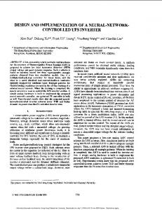
processing nodes by J.A.Samath and et al.[ J.A. Samath, P.S. Kumar and A. Begum 2010]. ANNs operate by breaking down complex problems to several easier ones .When properly trained , ANNs are often able to generalize i.e. to produce reasonable output even for input signals that were not part of the training set .Another advantage of ANNs is that they are robust to noise since their units are based upon a sum of several weighted signals ,oscillations in the individual values of these signals do not drastically affect the behavior of the network [ Annie Bjork 2005]. These advantages are very important for signal processing design, for more properly, in our RC circuit that have been designed. There are two types of artificial neural network, feed-forward and recurrent neural network . Figure(1) shows these two types of ANNs[Jaeger 2002].

(a)

(b)

Fig.1:Typical structure of a feed-forward network in (a) and a recurrent network (b) The two types depend on the connection patterns. In feed-forward neural network, all data flows in a network in which no cycles are present. And it is also called static neural network and it means that the neural network behavior depends only on the current input network . (Perceptron , Redial Basic Function ,Back-propagation ,etc) are examples to the feed-forward neural network. On the other hand, recurrent neural network has a cycle that can be connected from output of hidden unit to the input of this unit in a fashion depending on the type of the network . Recurrent neural network has feed-back connections with delays and it also called dynamic neural network which means that the neural network behavior depends not only on the current input (as in feed-forward networks) but also on the previous operations of the network .(Hopfield, Boltzman, Elman, etc) are examples of recurrent neural network. Unlike the recurrent nets with symmetric weights or the feed-forward nets, these nets do not necessarily produce a steady-state output . Several neural networks have been developed to learn sequential or time- varying patterns, RNN can be classified in two categories : partially and fully recurrent . Two of the well-known partially RNNs are Elman and Jordan networks [Laurene Fausett 2006]. In this paper, we used Elman neural network to design differentiation circuit which consist of a resistor with a capacitor .The efficiency of the Elman network structure is limited to low order systems due to the Elman network that had failed in identifying even second order linear systems as reported in the references insufficient memory[Adem Kalinli And Seref Sagiroglu 2006] .Our RC circuit is a first order linear system, therefore. the Elman neural network can implement the behavior of RC circuit.

1029


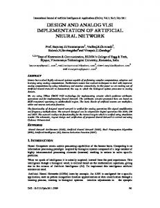
This paper is divided into five major sections. Besides this introductory section, section II describes Simple Recurrent Network (SRN), section III describes the proposed design and training of Elman neural network, section IV presents the results that we obtained after training the designed network . Finally, section V gives the conclusions. II. PARTIALLY RECURRENT NEURAL NETWORK Elman Neural Network (Simple Recurrent Network (SRN)) RNNS can generate and store temporal information and sequential signals. A commonly used recurrent architecture is the Elman model [Cornelius T. Leonde 1998]. Figure(2) shows the layer of Elman, which acts as a short-term memory in the system.

Output layer

Hidden layer

Context layer

Input layer

Fig.2: Elman neural network From the figure, we can define the Elman neural network as a feed forward network in addition to context layer. The number of context layers is equal to the number of hidden layers. The context layer has the same neurons that have been used in hidden layer because it is used as memory that have a copy of the output of hidden layer . Therefore, the output of hidden layer is fed directly to the input of context layer without any weight. the output of the context layer that fed to the hidden layer is weighted. Context layer here works as short term memory. It is remembering the output from the hidden layer and feed the value of the previous error in the hidden layer [http://zone.ni.com/devzone/cda/tut/p/id/2811]. The simple recurrent net is Elman neural network. It is a two-layer backpropagation network , with addition of feed-back connection from the output of hidden layer to its input . Due to this feed- back path, the Elman networks learn to recognize and generate temporal patterns , as well as spatial patterns. Figure(3) shows two-layer Elman network [YU HEN HU JENQ-NENG HWANG 2007]. .

1030

Fig.3: Example of two-layered Elman network [10] In other words , this recurrent connection allows the Elman network to detect and generate time-varying patterns and it is also can store information for future references. All these features of the network are important for designing electronic circuit. Therefore, this type of network have been used in our RC design . III. THE PROPOSED DESIGN AND TRAINING OF THE NETWORK RC circuit have been considered so that the NN simulates its behaviour. There may be significant advantages of this approach as compared to conventional methods such as: real time compensation for component change with temperature, prediction control (which means that we can predict the performance of electronic circuit , need less resources flexibility to control, etc. Electronic networks possess the flexibility to model all linear and nonlinear phenomena. Because of this flexibility, they will often represent working physical models of neural networks [JACEK M. ZURADA 1992]. The electronic circuit that have been considered is shown in figure (4):

The differential equations relating Vin and Vout , the output and the input voltage , respectively , which describes the behaviour of the RC circuit, is (1) d (vin  vout ) Vout  RC dt

(2)

Eq.(2) was built by simulink (MATLAB simulation program) to explore the input/output values for different input waveforms in order to use this data to train the RNN. The simulation model of equation (2) as shown in Fig(5) consists mainly of differentiator and amplifier of gain=RC.

1031


Fig.5:RC circuit in simulink As mentioned earlier , we used Elman network to design the RC circuit. The designed NN consists of three-layers (2-recurrent layers and one output layer). Fig(6) shows the structures of the designed NN. Del

Del

linear weight 1

linear weight 2

Input

Bia

Bi

Bia

1 Input

linear

Weig

1

1 Recurrent layer1

Recurrent

Output layer

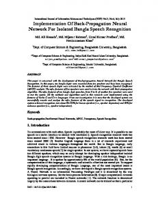
Fig.6: Three-layer Elman network At the beginning, the network is trained when the inputs of the RC circuits are (sine, square and triangular) waves. Fig(7) and Fig(8) show the input/output waveforms that are the results of the model of Fig(5) and are trained on by the designed RNN of Fig(6). IV. RESULTS In this section , we can see all expected results of the designed neural network after training. Also, the waveforms of the input and the output of the RC circuit, which represents the training set and the target of the neural network or the waveforms before training are presented. And then, after training the neural network it is tested by feeding different waveforms (sinusoidal, triangular and square waves), and then the network outputs are compared with the outputs of the real RC circuit. Firstly ,figure (7-a) shows the input and the output of the RC circuit. It is clear that for sine function input, the output is a cosine function. Samples of these two waves with rates greater than Nyquist rate are trained by the RNN. Fig(7-b) shows the input and the output waveforms of the RNN after training when the network is tested by sine function input. It is quite clear that the RNN acts as the RC circuit.

1032

(a)

(b) Fig.7: The input sine wave and the output is cosine wave (a) training signals (RC input/output) and (b) test signals (network input/output) In figures (8-a),(9-a), (square and triangular waveforms) represent the inputs and (impulse and square waveforms) represent the outputs of the RC circuit respectively. While in figures (8-b),(9-b) the same waveforms are coming out from the RNN after training.

(a)

(b)

Fig.8: The input is square wave and the output is impulse wave (a) training signals (RC input/output) and (b) test signals (network input/output)

(a) (b) Fig.9: The input is triangular wave and the output is square wave (a) training signals (RC input/output) and (b) test signals (network input/output)

1033


The final design of the neural network has 12 neurons in first recurrent layer , 22 neurons in the second recurrent layer and one neuron in output layer. In MATLAB, the training function is 'traingdx' and the performance function is 'mse' , the learning rate was chosen (lr min=0.0027 ,lr max=0.5566) , goal=0 and no. of epochs=70000. The performance goal was eventually met at epoch 69977. At the last the final design of the RNN is trained on all types of signals(sine, triangular and square) all together. Figure(10-a) shows the training signals that are coming out from the RC circuit, and figure(10-b) shows the input/output of the RNN after training. It is clear that the RNN generates the same waveforms that is output from the RC circuits when both have the same inputs. Table (1) shows the comparison of the some samples of the training and operating data. The Mean square error squared is found to be (MSE = =1.243*

), and RMS of error is (RMSE=

=0.01114899) volt.

(a)

(b) Fig.10: Many inputs waveforms (a) training signals (RC input/output) and (b) test signals (network input/output) Table (1): Comparison between some samples of training data and neural network results Vout  RC

S.No 1 2 3 4 5 6 7 8 9 10 11 12 13 14

15

Input sample voltage (volt) 0 0.1837 0.3646 0.5326 0.6818 0.8068 0.9032 0.9676 0.9978 0.9926 0.9522 0.8781 0.7729 0.6403

0.4851

d ( vin  vout ) dt

RC output voltage (volt) 0.3729 0.3707 0.3513 0.3194 0.2763 0.2233 0.1624 0.0958 0.0258 -0.0451 -0.1145 -0.1797 -0.2387 -0.2891

NN output voltage (result) 0.3729 0.3707 0.3515 0.3198 0.2761 0.2234 0.1633 0.0974 0.0202 -0.0464 -0.1051 -0.1603 -0.2436 -0.3037

4* 1.6* 4* 1* 8.1* 2.56* 3.136* 1.69* 8.836* 3.7636* 2.401* 2.1316*

-0.3293

-0.3379

7.396*

1034

0 0

It is obvious now that any circuit can be trained by the designed RNN. And then the RNN works the same as the circuit. There are many advantages when having a redundant circuit. One of them is to find the fault when happens in the real circuit. Another advantage is to make a compensation when there is a drift in the output.

Fig.11: NN on line training connections V. CONCLUSIONS This work successfully presents a design of electronic circuit simulator which is a simple recurrent network (SRN). The same network structure can be used to learn the input/output behaviour of any other circuits. The difference is only the weights of the neurons which are being fixed after training on the circuit under consideration. By using NN to simulate electrical circuits, it can be used to detect faults and achieve compensation if there is any drift in the characteristics of the circuit. The NN used in this work has two probes that can detect two points in any circuit. If it is required that the NN has to have more than two probes, another NN structure has to be designed. Mainly, other context layers are required. VI. REFERENCES Adem Kalinli And Seref Sagiroglu, "Elman Neural Network with Embedded Memory For System Identification" , Journal Of Information Science And Engineering 22, pp.1555- 1568,2006. Annie Bjork, Generation of Recurrent Neural Networks Using an EvolutionaryMethod Inspired by Gene Regulation In Biological Organisms", Chalmers University of Technology, Department of Applied Mechanics , 2005. Cornelius T. Leonde, "Neural Network Systems Techniques and Applications ", Vol. 3, "Implementation Techniques", Academic Press ,San Dieg, California, 1998. G. L. Dempsey, "A New Design Strategy for the Tank and Hopfield Neural Analog-to-Digital Converter , Bradley University, 1058-6393/93 $03.00 1993, IEEE ,pp 375-380. H. Jaeger, “Tutorial on training recurrent neural networks, covering BPPT,RTRL, EKF and the "echo state network" approach”, German National Research Center for Information Technology, International University Bremen, GMD Report 159, 2002. Available at http://www.pdx.edu/sites/www.pdx.edu.sysc/files/Jaeger_TrainingRNNsTutorial.200 5.pdf

1035


http://zone.ni.com/devzone/cda/tut/p/id/2811. JACEK M. ZURADA, "Introduction To Artificial Neural Systems", by West Publishing Company, New York, ISBN 0-314-93391-3 ,1992. J.A. Samath, P.S. Kumar and A. Begum, “Solution of Linear Electrical Circuit Problem using Neural Networks”, International Journal of Computer Applications (0975 – 8887), Vol. 2, No.1, pp.6-13, May 2010. Laurene Fausett, "Fundamentals Of Neural Networks", ISBN 10: 0133341860 / 013-334186-0,ISBN 13: 9780133341867. Sukumar Kamalasadan, "A New Generation of Adaptive Control: An Intelligent Supervisory Loop Approach", University of Toledo, Department of Electrical Engineering and Computer Science, August 2004. Yu Hen Hu and Jenq-Neng Hwang, "Hand Book of Intelligent Systems And Signal Processing In Power Engineering ", Springer-Verlag Berlin Heidelberg, Boca Raton, ISBN 0-8493-2359-2, 2007. Z.Zhang, "Training Elman Neural Network For Dynamic System Identification Using An Adaptive Local Search Algorithm "ICICInternational, ISSN13494198, Vol. 6, No.5, pp. 2233-2243,May 2010.

1036