Journal of Clean Energy Technologies, Vol. 1, No. 4, October 2013
Neural Network Output Partitioning Based on Correlation Shang Yang, Sheng-Uei Guan, Shu Juan Guo, Lin Fan Zhao, Wei Fan Li, and Hong Xia Xue
II. CONSTRUCTIVE BACK PROPAGATION (CBP) NEURAL NETWORK ALGORITHM
Abstract—In this paper, an output partitioning algorithm is proposed to improve the performance of neural network (NN) learning. It is assumed that negative interaction among output attributes may lower training accuracy when we have only one single network to produce all the outputs. Our output partitioning algorithm partitions the output space into multiple groups according to correlation, with strong correlation within each group. After partitioning, each group employs a learner to train itself. The training results from each group are integrated to produce the final result. According to our experimental results, the accuracy of NN is improved.
Constructive Learning Algorithm consist of Dynamic Node Creation method [3], Cascade-Correlation [4] as well as its variations [5]-[7], Constructive Single-Hidden-Layer Network [8] and Constructive Back propagation [9] (CBP). CBP is used for our work, a summary of which [9] follows. A. Step1. Initialization The network is initialized with only random weights and connections from the input units to the output units. The weight of the initialized network will be trained by minimizing the error with the function:
Index Terms—Output attributes, partition, correlation, interference, neural network.
=∑
I. INTRODUCTION As a useful machine-learning tool, Neural Network (NN) is often employed in solving classification [1] and regression problems. Partitioning of the output space is to place output attributes in different groups and train each group with different sub-networks [2]. In conventional neural networks, there is no partitioning of the output space. In this paper, it is assumed that there may exist interferences among different outputs, leading to the poor performance of neural network training. Beyond interference, we will also benefit from the positive interaction among output attributes, thus promotion. Inspired from this observation, a new algorithm for NN training is designed. This algorithm aims at reducing interference while maximizing the effect of promotion. Output attributes are put into different groups with each group to be trained individually. To tackle the drawbacks such as low accuracy and weak generalization, we introduce ensemble learning to integrate the results from different groups. In the second section, we introduce the CBP network and its growing algorithm. In section 3, the sub-network model is presented, followed by a detailed presentation of the output partitioning algorithm in section 4. Some experimental results are presented in section 5. Finally, section 6 has the conclusion.
−
(
(1)
)
In the formula, P is the number of training sample and K is the number of output units. and respectively stand for the actual output value and desired output value of the pth training sample at the kth output units. B. Step2. Train a New Hidden Unit Add the ith new hidden unit. Connect input units to the ith new hidden unit then connect it to the output units. Adjust all the weights connected to the new hidden unit with the function (minimizing the error): =∑
∑
∑
+
−
(2)
where a is the activation function. wjk is the connection from jth hidden unit to kth output unit with the weights. C. Step3. Freeze the New Hidden Unit Fix the weights associated with the hidden unit forever. D. Step4. Test for Convergence If the current number of hidden units is able to solve the problem, stop. Otherwise, continue with step 2.
III. SUB-GROUP MODEL OF INPUT ATTRIBUTES A. Output Partitioning Model The output space is partitioned into r sub-groups, with each consisting of all the input attributes while generating at least one output. Thus, formula (1-1) can be transformed into:
Manuscript received December 28, 2012; revised February 22, 2013. This research is supported by the National Natural Science Foundation of China under Grant 61070085 (e-amil:
[email protected]) Shang Yang, Sheng-Uei Guan, Shujuan Guo and Hong Xia Xue are with the School of Electronic & Information Engineering, Xi’an Jiaotong University, Xi’an, China (e-mail:
[email protected]) Lin Fan Zhao and Wei Fan Li are with the Dept. of Computer Science and Software Engineering, Xi’an Jiaotong-Liverpool University, Suzhou, China.
DOI: 10.7763/JOCET.2013.V1.78
∑
=
342
−
Journal of Clean Energy Technologies, Vol. 1, No. 4, October 2013
=∑
∑
(
) +∑
− ⋯+∑
(
− (
⋯
minimum so far is defined as the generalization loss at epoch t:
) +
−
)
( )
( ) = 100( =∑
∑
+∑
−
) +…+∑
∑
(
+
∑
+⋯+
=
(3)
)
(6)
− 1)
The training will stop if the generalization loss is too high. Otherwise, it will result in over fitting. A training strip of length m [10] is defined as the sequence of m times repeat from n+1 to n+m. Especially, n is divisible by m. During the training strip, training progress is measured by Pm (t): it means how much larger the average error is than the minimum.
−
⋯
( )
−
B. Sub-Network Model Sub-NN1, sub-NN2, sub-NNr replace the original network after grouping. These sub-networks are trained by CBP. Each sub-NN produces only a fraction of the result. And the final result is generated by integrating the sub-networks by some ensemble learning method.
( ) = 1000(
∑ ∈
,… ∈
,…
( )
− 1)
(7)
B. Procedure for Sub-Network Training and Growing The picture 4-1 shows the procedure for sub-network training and growing. sub-epoch stands for the number of epochs for training one neural network. Totale poch represents the total number of epochs of growing the whole neural network.
Fig. 1. Output attribute sub-network model
IV. OUTPUT PARTITIONING BASED ON CORRELATION A. Definitions CBP neural networks are very sensitive to the change of training time. If training time is too short, the neural network won’t be able to produce good result. However, long training will result in over fitting and poor bad generalization. In this article, the validation set is applied to determine the training time [10], [11]. A dataset is divided into three sub dataset: a training set is used to train the network; a validation set is used to evaluate the quality of the network to avoid over fitting during the training; finally, a test set is used to evaluate the resultant network. In this paper, the size of training, validation and test size is 50%, 25% and 25% of the dataset’s total available patterns. Training error E is mean square error percentage [10]. It is used to reduce the number of the coefficients in formula (1-1) and dependence on the range of output values. = 100
∑
∑
(
−
)
Fig. 2. The produce for growing and training sub-network
C. Correlation Partitioning Algorithm The purpose of output partitioning is to take advantage the relation among the outputs and to reduce the high internal interference. By dividing, we can avoid the internal interference. By partitioning, we can make use of the potential relationship. Here we propose an output partitioning algorithm based on correlation to produce. The details of this algorithm are described as follows: Step 1: Calculate the correlation of every two output attributes. And take the absolute values of the correlation. Step 2: List all output attribute pairs in descending/ascending orders. Step 3: For the two attributes in the same pair, if they weren’t grouped in any existing partition, form a new partition with these two outputs attributes only. Step 4: If these two output attributes have been partitioned already, then skip this pair. Step 5: If only one of the output attribute has been partitioned, the other one should be considered if it can be placed into the existing partition in the prescribed order. If and only if an incoming output attribute has strong correlation with all of the attributes in the partition, it can be placed into this partition. Once an attribute is assigned into a
(4)
In the above formula, and are the maximum and minimum output values in formula (1-1). (t) is per pattern’s average error of After epoch t, training network. ( ) is the corresponding error on validation set and it is used to determine the time to stop training. Also, ( ) is the test error and is used to describe the quality of the network. (t) stands for the minimum validation error from the start to epoch t. ( ) = min
( ′)
(5)
The relative increase of the validation error over the 343
Journal of Clean Energy Technologies, Vol. 1, No. 4, October 2013
UCI machine learning repository. This dataset consists of 7200 patterns with has 21 inputs and 3 outputs.
partition, the other partitions should not be considered. Otherwise form a new partition for it. If the correlation coefficient is less than 0.1, it can be regarded as having no correlation.
TABLE III: THYROID OUTPUT CORRELATION COEFFICIENTS 1 2 3 Output No.
V. EXPERIMENTAL RESULTS In this paper, we use the Rprop algorithm for training the sub-NNs. The parameters used in the algorithm are below: ƞ = 1.2, ƞ = 0.5 , ∆ = 0.1, ∆ = 50 , ∆ = 1.0 − 6. All the units use the sigmoid activation function. The experiments were simulated on a Pentium(R) Dual-Core E5800. The result of all experiments is the average value of results over 20 times.
1
2
-0.517**
1
3
-0.231*
-0.256**
1
4
-0.094
-0.105
-0.047
1
5
-0.116
-0.129
-0.057
-0.023
1
6
-0.307**
-0.341**
-0.152
-0.062
-0.076
Full-partitioni ng
36.13
Ascending order
{1,2,3}{4} {5}{6}
32.06
Descending order
{1,2,6}{3} {4}{5}
32.93
45.28
43.40
38.81
3
-0.563**
-0.805**
1
Non-partiti oning Full-partitio ning Ascending order Descending order
Classificatio n error
Max error
Min error
1.86
2.17
1.61
1.89
2.11
1.56
{1,3}{2}
1.72
1.93
1.31
{2,3}{1}
2.06
2.33
1.73
Std deviation 0.16 0.15 0.22 0.18
C. Flare Flare is also taken form UCI and is a regression problem. So, there is no the classification error any more. We apply the test error to judge the network’s performance. It has 24 inputs, 3 outputs and 1066 patterns.
1
TABLE V: FLARE OUTPUT CORRELATION COEFFICIENTS Output No. 1 2 3
TABLE II: EXPERIMENTAL RESULTS OF GLASS Partition Classifica Max Min result tion error error error 47.17
1
Partition results
The average correlation is 0.168. The list of descending-correlation-order pairs is: {1,2}-{2,6}-{1,6}-{2,3}-{1,3}. The ascending-order list is: {1,3}-{2,3}-{1,6}-{2,6}-{1,2}. The corresponding partitioning results are {1,2,6}{3}{4}{5} and {1,2,3}{4}{5}{6}.
41.22
-0.037*
TABLE IV: EXPERIMENTAL RESULTS OF THYROID
*. Significantly correlated in level .05 (both sides). **. Significantly correlated in level .01 (both sides).
Non-partition ing
2
The average correlation is 0.468. The list of descending-correlation-order pairs is: {2,3}-{1,3}. The ascending-order list is: {1,3}-{2,3}. The corresponding partition results are: {1,3}{2} and {2,3}{1}.
6
1
1
*. Significantly correlated in level .05 (both sides). **. Significantly correlated in level .01 (both sides).
A. Glass The glass dataset is taken from the UCI machine learning repository. Classification error (rate) is regarded as judgment standard. It has 9 inputs, 6 outputs and 214 patterns. This dataset is used to classify glass types. TABLE I: GLASS OUTPUT CORRELATION COEFFICIENTS 2 3 4 5 Output No. 1
1
33.96
26.42
27.51
25.50
1
1
2
0.082
1
3
0.050
0.472**
1
*. Significantly correlated in level .05 (both sides). **. Significantly correlated in level .01 (both sides). TABLE VI: EXPERIMENTAL RESULTS OF FLARE Std Test Max Min deviation Partition error error error
Std deviation 4.31
4.63
3.48
3.97
Non-partitioning
0.56
0.68
0.52
Full-partitioning
0.55
0.60
0.53
Ascending order
{2,3}{1}
0.52
0.63
0.51
Descending order
{2,3}{1}
0.52
0.63
0.51
0.034 0.015 0.023 0.023
D. Pollution This dataset is taken from Carnegie Mellon University. It is a regression problem with 6 inputs, 5 outputs and 508 patterns.
B. Thyroid Thyroid is a classification problem and is taken from the 344
Journal of Clean Energy Technologies, Vol. 1, No. 4, October 2013 TABLE VII: POLLUTION OUTPUT CORRELATION COEFFICIENTS Output 1 2 3 4 5 No. 1
1
2
-0.12**
3
-0.35
**
-0.33
**
-0.43
**
4 5
difficult to distinguish from one another. Partitioning can also help resolve internal interference [12] inherent inside large networks. REFERENCE
1
[1]
0.47
**
1
0.27
**
0.73**
0.44
**
**
0.92
1
[2]
0.61
**
1 [3]
*. Significantly correlated in level .05 (both sides). **. Significantly correlated in level .01 (both sides).
[4]
The average correlation is 0.467. The list of descending-order-correlation pairs is: {3,5}-{3,4}-{4,5}-{2,3}. The ascending-order list is: {2,3}-{4,5}-{3,4}-{3,5}. The corresponding partition results are:{3,4,5}{1}{2} and {2,3}{4,5}{1}.
[5] [6] [7]
TABLE VIII: EXPERIMENTAL RESULTS OF POLLUTION Partition Test Max Min Std result error error error deviation Non-partitioning
0.64
0.70
0.56
0.036
Full-Partitioning
0.62
0.66
0.54
0.029
[8] [9] [10] [11]
Ascending order
{2,3}{4,5}{1}
0.60
0.65
0.52
0.039
Descending order
{3,4,5}{1}{2}
0.61
0.68
0.55
0.033
[12] [13] [14]
VI. CONCLUSION
[15]
This paper presented a new approach to output partitioning based on correlation. A problem can be divided into several sub-problems where each is responsible for a fraction of the outputs. Either for classification or regression, the results is inspiring. It is easy to understand. If there is strong correlation between two outputs, it means that there exist similarities between the two outputs. By training two strongly correlated outputs together, we can simplify the original problem. Also, if there exists no correlation between the outputs, it may imply that each of the outputs is
345
R. Anand, K. Mehrotra, C. K. Mohan, and S. Ranka, “Efficient classification for multiclass problems using modular neural networks,” IEEE Trans. Neural Networks, vol. 6, no. 1, pp. 117–124, 1995. S. U. Guan and S. Chun Li, “Parallel Growing and Training of Neural Networks Using Output Parallelism,” IEEE Trans on Neural Networks, vol. 13, no. 3, May 2002 T. Ash, “Dynamic node creation in backpropagation networks,” Connection Sci., vol. 1, 1989, pp. 365–375. S. E. Fahlman and C. Lebiere, “The cascade-correlation learning architecture,” Advances in Neural Information Processing systems, vol. 2, 1990, San Mateo, CA: Morgan Kaufmann, pp. 524–532. L. Prechelt, “Investigation of the CasCor family of learning algorithms,” Neural Networks, vol. 10, 1997, pp. 885–896. M. Setnes and H. Roubos, “GA-fuzzy modeling and classification: complexity and performance,” IEEE Trans. Fuzzy Syst., vol. 8, no. 5, pp. 509–522, 2000 S. U. Guan and S. Li, “An approach to parallel growing and training of neural networks,” in Proc. 2000 IEEE Int. Symp. Intell. Signal Processing Commun. Syst. (ISPACS2000), Honolulu, HI. D. Y. Yeung, “A neural network approach to constructive induction,” in Proc. 8th Int. Workshop Machine Learning, Evanston, IL, 1991. M. Lehtokangas, “Modeling with constructive backpropagation,” Neural Networks, vol. 12, 1999, pp.707–716. L. Prechelt, A set of neural network benchmark problems and benchmarking rules, Technical Report 21/94, Department of Informatics, University of Karlsruhe, Germany, 1994. L. Rechelt, “Investigation of the CasCor family of learning algorithms,” Neural Networks, vol.10, no. 5, pp. 885–896, 1997 R. A. Jacobs, M. I. Jordan, M. I. Nowlan, and G. E. Hinton, “Adaptive mixtures of local experts,” Neural Comput., vol. 3, no. 1, pp. 79–87, 1991. S. U. Guan and Y. Qi, “Output partitioning of neural networks,” Neurocomputing, vol. 68, 2005, pp. 38–53. R. A. Jacobs, M. I. Jordan et al., “Adaptive mixtures of local experts,” Neural Comput, vol. 3, no. 1, pp. 79–87. E. B. Baum and D. Haussler, “What size net gives valid generalization?” Neural Comput., vol. 1, no. 1, pp. 151–160, 1989.
Sheng-Uei Guan received his M.Sc. & Ph.D. from the University of North Carolina at Chapel Hill. He is currently a professor in the computer science and software engineering department at Xi'an Jiaotong-Liverpool University (XJTLU). He is also affiliated with Xi’an Jiaotong University as an adjunct faculty staff. Before joining XJTLU, he was a professor and chair in intelligent systems at Brunel University, UK.